Unconventional Well Test Analysis for Assessing Individual Fracture Stages through Post-Treatment Pressure Falloffs: Case Study

Abstract

Researchers and operators have recently become interested in the individual stage optimization of unconventional reservoir hydraulic fracture. These professionals aim to maximize well performance during an unconventional well’s early-stage and potential Enhanced Oil Recovery (EOR) lifespan. Although there have been advances in hydraulic fracturing technology that allow for the creation of large stimulated reservoir volumes (SRVs), it may not be optimal to use the same treatment design for all stages of a well or many wells in an area. We present a comprehensive review of the main approaches used to discuss applicability, pros and cons, and a detailed comparison between different methodologies. Our research outlines a combination of the Diagnostic Fracture Injection Test (DFIT) and falloff pressure analysis, which can help to design intelligent production and improve well performance. Our field study presents an unconventional well to explain the objective optimization workflow. The analysis indicates that most of the fracturing fluid was leaked off through natural fracture surface area and resulted in the estimation of larger values compared to the hydraulic fracture calculated area. These phenomena might represent a secondary fracture set with a high fracture closure stress activated in neighbor stages that was not well-developed in other sections. The falloff pressure analysis provides significant and vital information, assisting operators in fully understanding models for fracture network characterization.

1. Introduction

The advent of unconventional reservoir development is a turning point in the global oil and gas industry, since these resources contain massive hydrocarbon reserves larger than those found in conventional formations. Domestic oil production from liquid-rich shale (LRS) reservoirs in North America has seen significant development, according to the US Energy Information and Administration (EIA), with production dramatically increasing in the ‘top producing’ American oil shale plays: the Bakken, Eagle Ford, and Permian Basin. This hydrocarbon production improvement has been driven by the application of modern horizontal drilling and multi-stage hydraulic fracturing (MSHF) techniques, which makes it possible to access low-porosity (<10%) and low-permeability (<0.1 mD) formations [1,2]. The creation of large stimulated reservoir volumes (SRVs) has been achieved through breakthroughs in hydraulic fracturing technology; however, fracture treatment is not necessarily effective [3]. Operators have started utilizing tighter spaced clusters, longer stage lengths, and greater proppant volumes in their stimulation designs [4,5]. The ultimate oil recovery reported by several studies is less than 8% due to a rapid decline in unconventional well performance, and by approximately 75% within the first two years of well production (Figure 1).

The decline is due to a low to no hydrocarbon recharge from the ultra-tight matrix blocks since the natural and induced fractures close, and there is a high flow resistance at the matrix–fracture interface; therefore, the increase in net stress leads to a zero-pressure gradient, which obstructs the fluid flow from the rock matrix into the fracture [3,6,7]. Proppant choice plays a significant role in fracture conductivity. An inappropriate choice may cause proppant deformation and/or crush under closure pressures. High-pressure drawdown may also cause formation rock compression, which leads to a reduction in matrix permeability with changes in reservoir pressure or stress [3,4,8]. The productivity of unconventional wells heavily relies on the effective fracture contact area or the propped fracture area per cluster, which is critical in evaluating hydraulic fracture treatment performance [9].

Performing a successful treatment design depends primarily on evaluating the stimulated formation before and during fracture treatment. Recommendations for the proper selection of slurry type and amount are provided to produce the optimal fracture geometry using a high-efficiency assessment [11]. Current literature suggests that the use of diagnostic tools is critical when assessing unconventional plays since they can reveal opportunities for future exploration, evaluation, delineation, and development [12]; however, currently available traditional methods are not feasible for decision-makers, even with the appropriate data. The majority of the previously published research is associated with high uncertainty and lacks a thorough discussion of fracture network characterizations. Only long-term production data were utilized in the past, the application of which caused ambiguity in understanding the hydraulic fracture performance [13,14]. This ambiguity was caused by the difficulty in utilizing conventional exploration and production techniques to establish commercial production rates [3,15].

Most of the previous post-treatment analysis studies of unconventional reservoirs do not provide quantitative discussions with detailed support case studies, and very few field studies have discussed the application of pressure falloff data [9]. We present guidelines to better understand unconventional well test analysis through critical literature reviews and case studies of fracturing treatment analysis to address the lack of quantitative evaluation.

We have concluded that post-stimulation condition performance evaluation using indirect methods, such as pressure falloff data, is the most promising technology. This approach may provide a clear perspective about the created fracture’s dimensions and properties; therefore, the effective fracture contact surface area for both natural and induced fractures can be determined from stage to stage during fracture treatment jobs. The application of pressure falloff data is a valuable tool that provides comprehensive information, such as the mechanics of the created open, closed, and propped hydraulic fractures, due to the tool’s capability of reflecting the rock and fluid’s physical behavior. This technology may overcome some limitations and weaknesses in most of the proposed techniques in the literature, such as production data analysis and micro-seismic methods.

2. Research Objectives

The main objective of diagnostic tool usage is to maximize well performance during both primary production and late-stage EOR processes by understanding the contribution of individual fracture stages [1,8,13]. Important pressure falloff data gathered after fracture treatments were generally ignored in the past, even though that detailed information could reveal attributes necessary for successful fracturing evaluation. There were also no precise measurement technologies for recording production rate and pressure during each stage to evaluate each cluster or stage’s contribution. The pressure falloff data tool has garnered significant interest in the oil and gas industry since it is a powerful method for defining prime fracture parameters to gain insight into the effectiveness of the treatment jobs’ fracture [9].

Evaluating fracture designs can be implemented on a stage-by-stage basis to optimize the overall performance of a well, unlike common performance evaluation methods such as Rate Transient Analysis (RTA) and micro-seismic fracture imaging/mapping (MS). We will investigate the following key parameters to evaluate these designs:

• The importance of closure stress, including closure behavior and geomechanics parameters, in fracture geometry and the impact of its variation from stage to stage.
• The variability of geology and mineralogy and their impacts on fracture propagation and geometry.
• The contribution of natural fractures in created well-reservoir contact areas and their impact on fracture geometry.
• The role of treatment designs on proppant distribution and characteristics, such as conductivity, crush, and embedment, which are related to closure stress and effective stress.
• Investigate if an optimal fracture contact area would exist for a specified treatment design.
• Identify optimal treatment design parameters for individual fracture stages, such as proppant volume and mesh size, fracturing fluid amount and type, and pump schedule.
• Prepare protocols for evaluating the success of individual fracture stages from the viewpoint of production performance, such as post-treatment analysis.
• Determine the contribution of individual fracture stages in the well’s overall performance and determine the right spot for treatment execution.
• Evaluate the lessons learned from fracturing in the previous stages. Develop a workflow for the real-time treatment design optimization for next-stage application to address good or bad frac-hits, unsuccessful designs, and fracturing in undesired formations.
• Determine if the expected treatment design optimization by stage would justify the additional cost and treatment design adjustments through case studies.

We have compared common fracture diagnostic tools, discussed DFIT and pressure falloff data, and analyzed fracturing treatment case studies fracturing for unconventional wells. We have also presented the potential of combining DFIT and pressure falloff data in various pressure-time plots to identify fracture and reservoir behavior characteristics. Guidelines to better understand unconventional well test analysis that can lead to real-time optimization and adjustment of fracture job treatments have been provided as we proceed from one stage to another in an MSHF operation.

3. Principle of Fracture Diagnostic Tools

Monitoring the growth of fracture networks in the subsurface is the common process during stimulation treatments in unconventional wells. The created fractures are usually simulated by simple bi-wing and single planar fracture model definitions, such as Perkins-Kern-Nordgren (PKN) and Khristianovic-Geertsma-de Klerk (KGD) fracture geometry models. These models assume that the hydraulic fractures will primarily stay within the pay zone and extend significantly [16]; however, in reality, the fracture networks can grow in an asymmetrical shape due to variable confinement across the geologic interfaces and orientation changes. Fracture growth around natural fractures can add more complexities to the fracture system due to the interaction between the induced and fissure networks [17]. An effective fracture network’s morphology in shale resources is still largely unknown. As a result of this knowledge gap and the network’s complexity, it is difficult to predict, obtain, and verify fracture geometry, such as fracture length, height, and containment. These challenges can lead to suboptimal outcomes when incorrect assumptions are used through fracture diagnostic applications [11].

There are several fracture diagnostic applications. These applications allow petroleum engineers to assess the success of the fracture stages and create optimal development strategies for effective reservoir drainage. These tools can also optimize the entire field development regarding well spacing and location, optimal design, and optimum interval/height coverage. Numerous fracture diagnostics are discussed by researchers that provide subsets of knowledge about treatment design optimization [13,18,19]: (a) direct far-field fracture diagnostic techniques, such as micro-seismic fracture mapping and tiltmeter, (b) direct near-wellbore fracture diagnostic techniques, such as production and temperature logging tools and radioactive tracers, and (c) indirect fracture-diagnostic techniques, such as transient pressure and rate transient analysis “PTA/RTA” and fracture modeling “net pressure analysis”.

We have focused on indirect fracture-diagnostic techniques in this review paper. Table 1 provides a brief discussion and comparison reference for widely used diagnostic tools with their strengths and limitations explained.

The analysis of source rock and fluid behaviors is detected by the fracture diagnostic tools, highlighting the fracture and reservoir properties; therefore, the combination of diagnostic tools provides more confidence and allows fracture engineers to make decisions in real-time. DFIT, post-treatment pressure falloff, micro-seismic, flowback, and other data can be collected and interpreted in real-time to assess the created contact surface areas and evaluate fracture design properties, such as fracture half-length, number of clusters, proppant loading, and fracture complexity and direction. The pump schedule can be adjusted from stage to stage by assessing the proppant placement and injection volumes to ensure the maximum pay zone proppant coverage. An optimal well stimulation strategy should be established to avoid some far-field issues, such as well interventions and frac-hits [11].

Applying the DFIT methodology and using post-treatment pressure falloff data as a fracture-diagnostic tool may assist us in monitoring the pressure interference and offset well intervention based on the survey comparison mentioned in Table 1. This technology will provide valuable information needed to improve individual fracture stage treatment design and enhance the production of the propped fracture surface area in real-time.

4. Diagnostic Fracture Injection Test (DFIT)

DFITs have been widely used in the oil and gas industry over the last 20 years. This approach is based on the pressure transient data procured immediately after fracture treatments to obtain a reliable assessment of fracture and reservoir properties. A DFIT is a standard well testing technique for ultra-low-permeability formations, where a traditional pressure transient test, such as a buildup test, is impractical. A DFIT analysis does not require a long shut-in time to reach the radial flow regime.

The pressure falloff data are analyzed in a DFIT to estimate the in-situ stress, fluid efficiency, leak-off coefficient, reservoir properties, and net pressure, which are the critical factors used to design and implement a successful main fracture treatment. A DFIT provides the representative properties of an undamaged formation since the test creates a large area of investigation that can extend beyond the damaged near-wellbore zone. The results from a DFIT can be used in several ways: (a) characterizing in-situ stresses and fracture compliance [20], (b) modeling hydraulic fracture propagation [21], (c) designing fracture treatment jobs [22], (d) modeling reservoir simulation [23], and (e) post-fracture treatment analysis [24]. This application can also be utilized in geologic carbon sequestration, nuclear waste repositories, and geothermal energy exploitation [17,25,26].

A DFIT implementation and interpretation should be studied in detail before any field execution or analysis. We have presented lessons learned and recommendations that may help operators design the optimum fracture jobs.

4.1. DFIT Design and Tactics

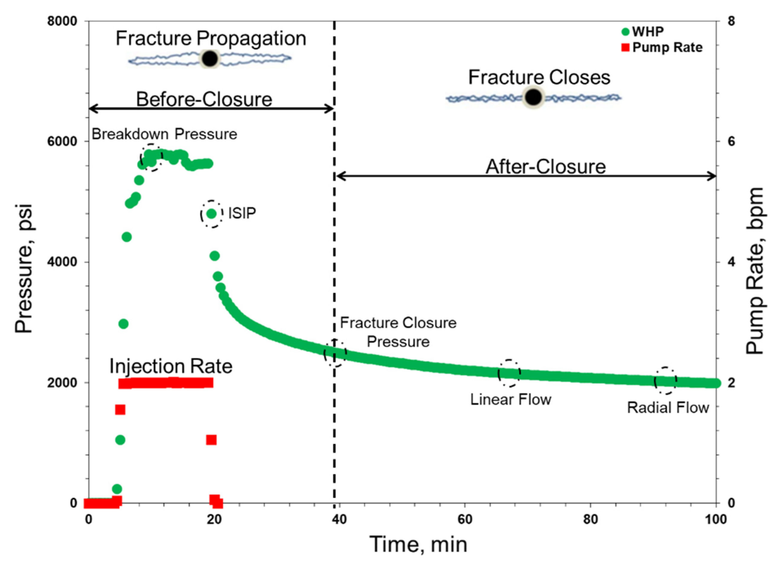
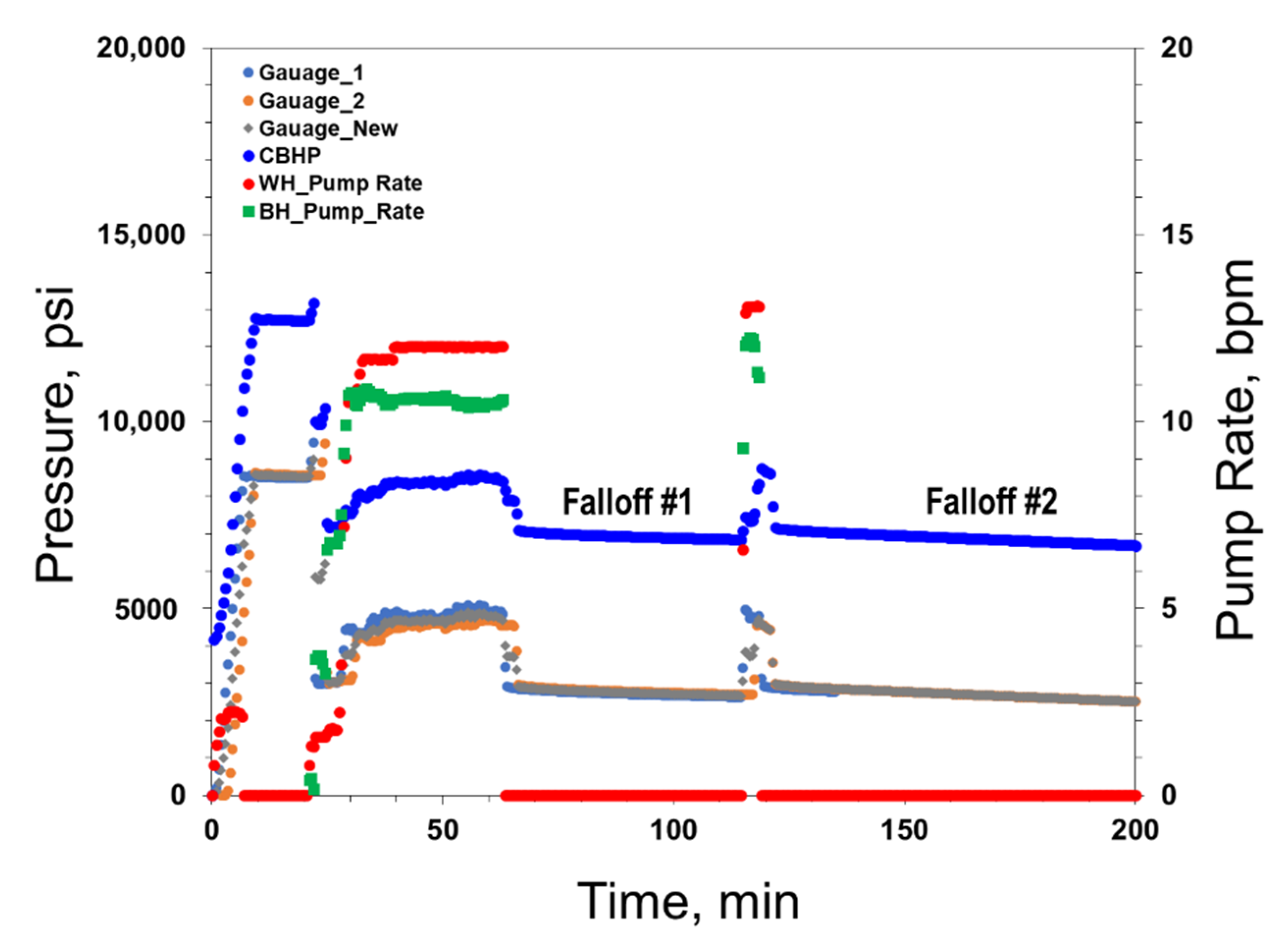
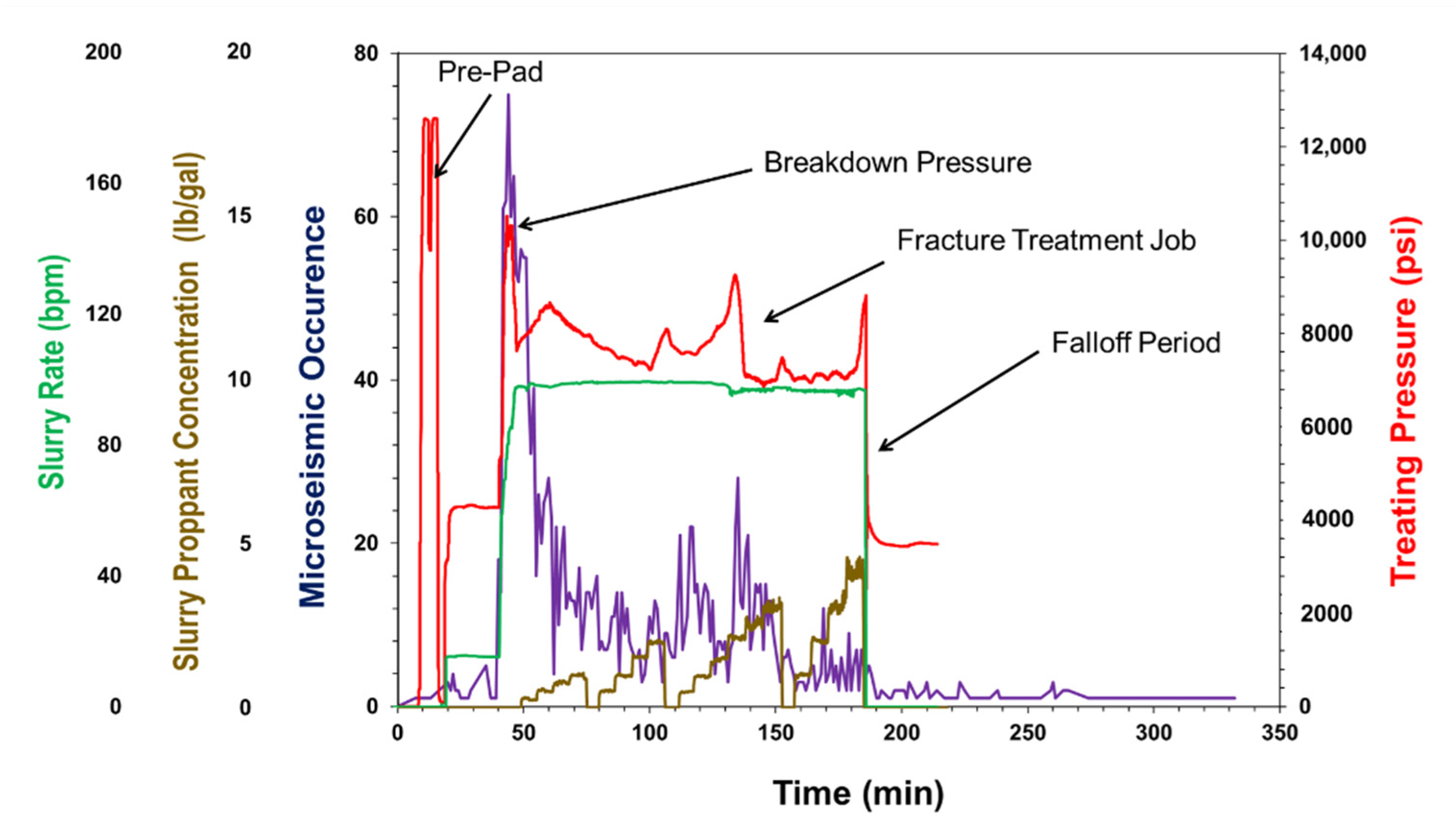
A typical DFIT operation pumps a small volume of the treatment fluid, such as water, without proppant at a constant rate for a short period of approximately 3–5 minutes. The injection pressure increases above the reservoir fracturing pressure, or breakdown pressure, creating a short artificial fracture in the target layer. The leak-off behavior is small during the injection period, and no filter cake forms on the fracture wall. The pressure falloff data is a recorded function during shut-in time immediately after the treatment. The injected fluid begins to leak-off into the formation until the fracture wall comes into contact, also called closure. The pressure falloff period recorded in the case studies we analyzed was extended for days or even weeks to observe the radial flow regime, depending on the reservoir characteristics.

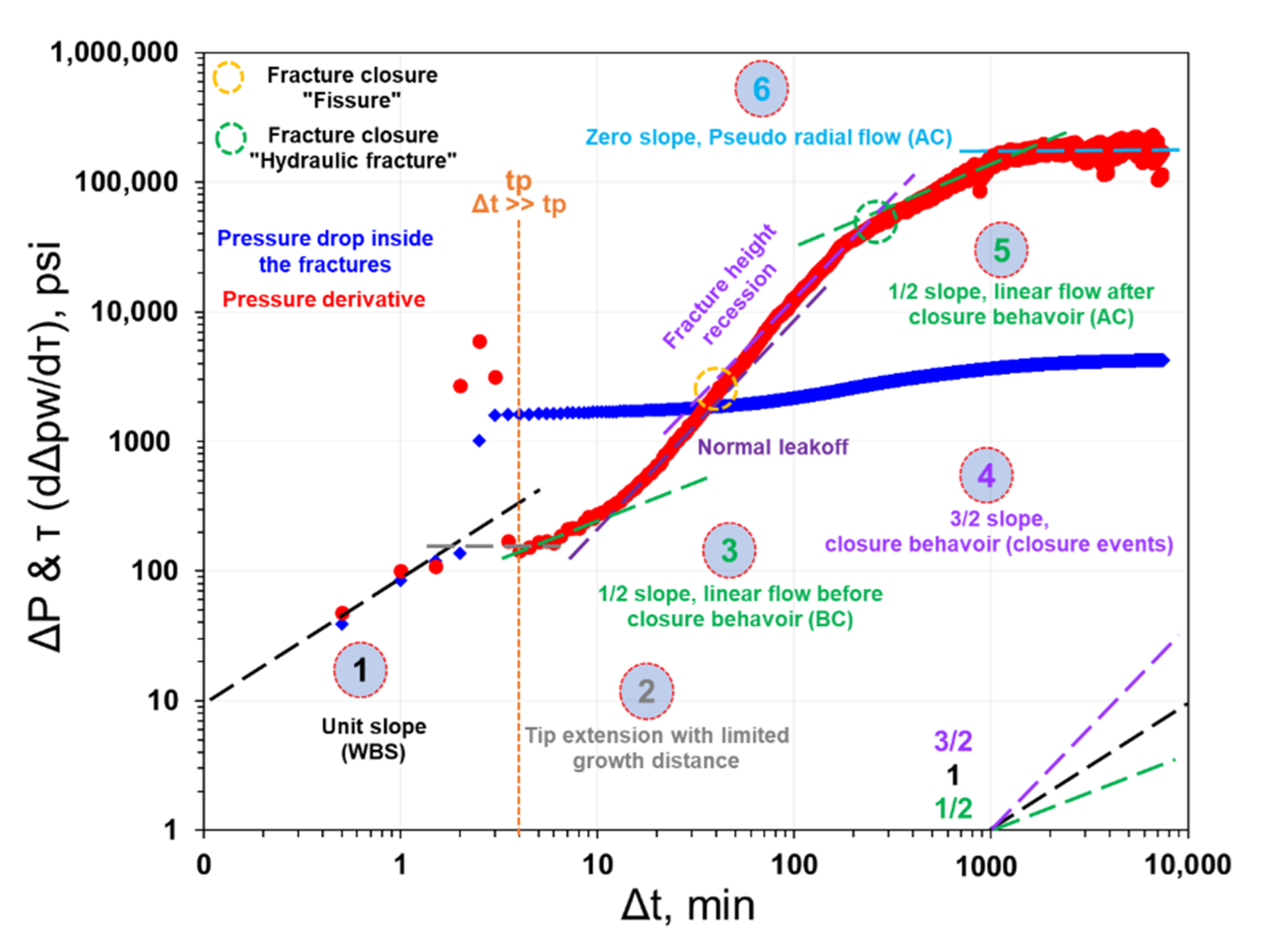
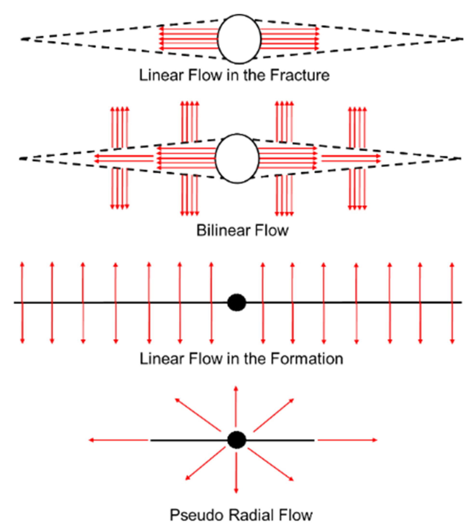
Figure 2 displays a typical pressure profile of a DFIT in the absence of natural fractures and weak planes. Two distinct periods of before and after closure (BC and AC) were analyzed to characterize the properties of the created fractures and reservoirs. These two periods were separated by the fracture closure event, which is the primary outcome and supplies us with the fracture closure pressure, or minimum in-situ stress. The fracture and reservoir properties were obtained by analyzing the typical flow regimes observed during the BC, before closure for fracture-dominated, and AC, after closure for reservoir-dominated, respectively (Figure 3).

The conditions of modeling in unconventional reservoirs are more complex than in conventional formations. Significant conflict exists on how to model the fracture closure behavior since most of the models assume that the fracture surface is perfectly smooth; however, fractures exist everywhere in the subsurface in the form of small-scale cracks and fissures, and large-scale joints and faults. The mechanical resistance and fluid transport properties found in unconventional formations are complicated and controlled by several factors, such as in-situ stress, compliance or stiffness, rock mineralogy, fracture-surface roughness, treatment fluid pressure inside the fractures, and leak-off rate [11,20,27]. A proper DFIT model must account for the effects of pressure-dependent leak-off and dynamic fracture compliance to precisely capture the fracture pressure response and obtain a realistic estimation of the fracture closure pressure and fluid leak-off behavior [20,28]. These parameters are crucial factors necessary for calculating the fracture surface contact areas to obtain proper hydraulic fracture modeling and accurate post-treatment assessment.

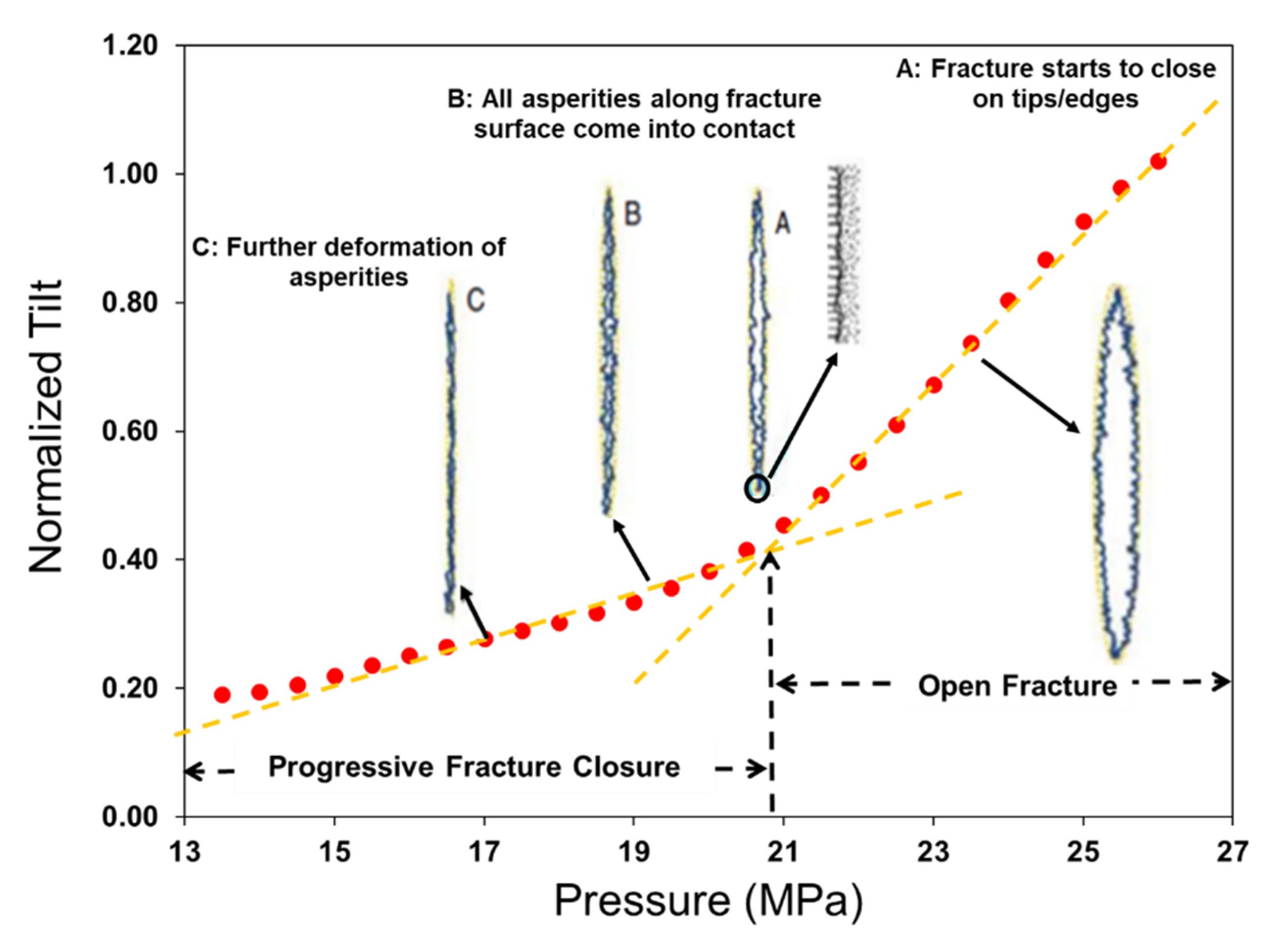
Investigating compelling field evidence using a downhole measurement that indicates what exactly occurs in the subsurface is paramount. Figure 4 illustrates the tiltmeter measurements of well #2B from the Gas Research Institute/Department of Energy M-site, which is defined as an indication of fracture displacement or fracture width [29].

Wang and Sharma [20] used recorded data to explain the relationship between normalized tilt and formation pressure (Figure 4). The data for this downhole field measurement were recorded and gathered immediately after the end of the several week-long test. The Y-axis presents the normalized tilt calculated by dividing each tiltmeter measurement by the maximum fracture displacement. The data were plotted vs. the wellbore pressure to generate the diagnostic plot (Figure 4), demonstrating a direct measurement of the rock deformation during the fracture closure behavior. The results indicate that the pressure falloff data response on a normalized tilt vs. formation pressure plot (Figure 4) is proportional to the fracture compliance (Equation (1), or inversely proportional to fracture stiffness, and the fracture closure behavior is a function of average displacement and fracture volume.

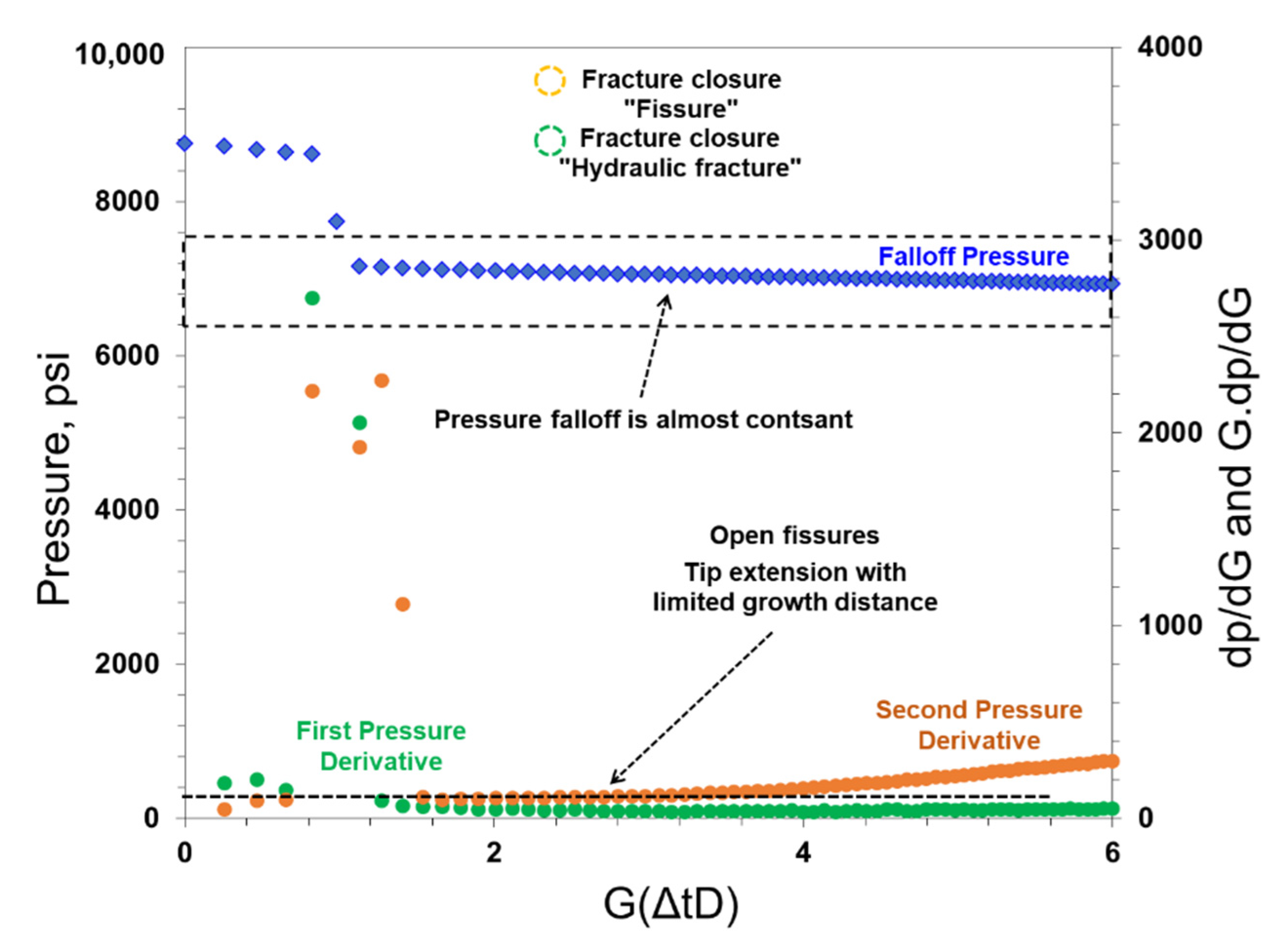
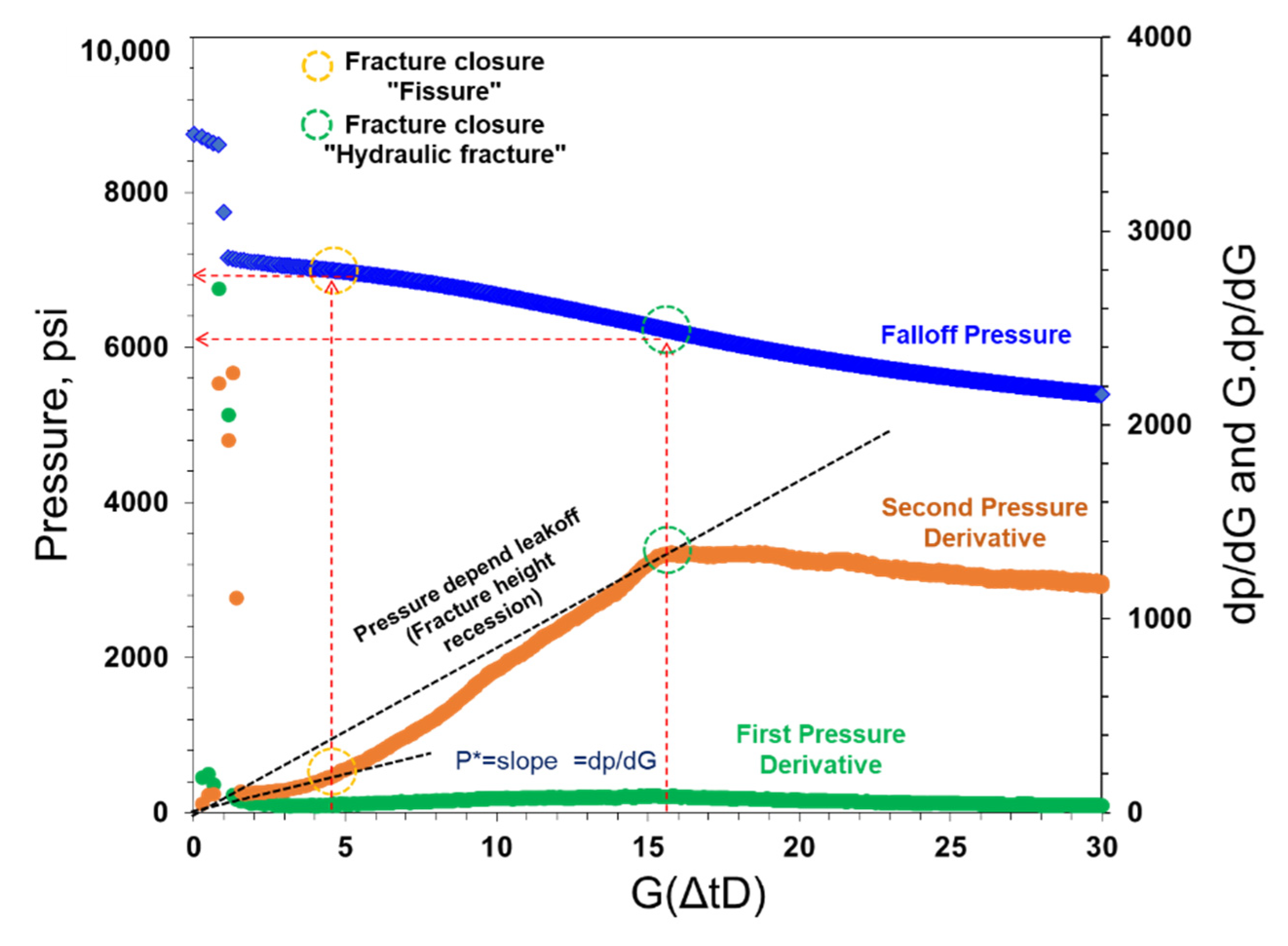
The fracture volume is proportional to the average fracture width as the pressure continues to decrease, and two distinct periods are indicated on the diagnostic plot: (1) The trend of the pressure falloff data is a linear decline until the point of measured pressure inside the fracture, or closure pressure, is greater than 21 MPa (3046 psi). At this point, the fractures are still open, the stiffness factor is constant, and the surface area remains constant until the fracture wall comes into contact, or closure. The fracture geometry can then be estimated directly using

Table 2. Fracture geometry models.

Fracture Model	PKN	KGD	Radial	Equation
$\mathrm{Area} \mathrm{exponent} \left(\alpha \right)$	4/5	2/3	8/9	-
$\mathrm{Fracture} \mathrm{compliance} \left(c_f\right)$	$\frac{\pi {\beta }_s{h}_f}{2E\prime }$	$\frac{\pi {\beta }_s{x}_f}{E\prime }$	$\frac{16{\beta }_s{R}_f}{3\pi E\prime }$	(1)
$g_0$	1.41	1.48	1.38	-
${\beta }_s$	4/5	0.9	3 π2/32	-

. (2) The pressure falloff data begin to deviate from a straight line at the inflection point on the plot, where the closure pressure is marked with a dashed green line; therefore, the fracture stiffness increases gradually, as a result of the fracture closure on the asperities of the fracture edges or tips (Table 1).

Table 1. Comparison of different diagnostic methods for fracture treatment performance analysis.

a. Production Data Analysis as a Diagnostic Method:
Pros	Cons	Results	Authors
The data are readily available at low costs, and their analysis is straightforward. This application is critical for using historical production data for various purposes: (a) Characterize reservoir and well stimulation properties, (b) Predict production performance for development plans and reserve estimations. Production data analysis is useful for checking the consistency of the data and identifying the flow regimes over time. There are a couple of ways to apply production data techniques: (a) Type curve analysis, (b) Straight line (flow regime) analysis, (c) Analytical and numerical simulation, (d) Empirical methods to quantify the hydraulic fracture performance at different unconventional well life stages. Production analysis is a tool to study linear flow regimes when assessing the productivity and effectiveness of completion designs. The impact of fracture-hit and offset stages can also be evaluated.	High-frequency measurements are required to obtain a reasonable analysis. The results suffering from some degree of uncertainty; therefore, more information is required, such as geology, phase behavior, and completion practices. This information needed is more complex compared to other approaches. Traditional production data analysis assumes that all clusters are similar, which appears to be an oversimplification of the problem. All production data analysis methods are non-uniqueness associated with well and reservoir properties; therefore, the different methods must be validated and cross-checked. The production data approaches for conventional rate transient methods need further modifications to analyze the MSHW data. Production data analysis does not offer any procedures for quick and measured adjustments of completion designs and production operations.	Fracture permeability. Conductivity. Storage coefficient. Fracture half-length. SRVs. Hydrocarbon in place. Reservoir permeability. Thickness product. Skin. Performance forecast.	[1,14,24,25,30,31]
b. Micro-Seismic Fracture Imaging/Mapping
Pros	Cons	Results	Authors
Micro-seismic imaging provides the best resolution and lowest uncertainties when characterizing fracture geometries in most cases. Micro-seismic mapping can be coupled with real-time simulations to accurately predict fracture growth in the target zone. This combination can be utilized to assess the effectiveness of flushing an unexpected screen-out, imaging proppant placement, synthetic micro-seismic event prediction, and fracture geometry control. Micro-seismic imagery is also helpful during postmortem well performance analysis to: (a) Calibrate numerical simulations, (b) Optimize stimulation design, (c) Investigate frac-hit phenomena, (d) Test new fracturing procedures, (e) Assess well drainage patterns, (f) Optimize economics, such as Net Present value (NPV) and Rate of Return (ROR).	This technology is not widely used due to its high cost. This application is associated with a few uncertainties due to source mechanisms: (a) Receiver-coupling resonances, such as improper sensor couplings with rock properties, including velocity-model limitations, formation anisotropy, noise, and mislocation. (b) The interference of fluid leak-off and stress effects in some formations, such as shale plays. Fracture geometries obtained from micro-seismic monitoring may not be accurate enough in certain situations; therefore, the geometries must be validated and cross-checked with other diagnostic tools. The extent of fractures parallel to the lateral might be difficult to interpret from micro-seismicity alone, such as in the case of micro-seismicity vs. dimensions. Micro-seismic imaging cannot provide accurate information on individual fractures and cracks, or whether they are open, closed, or propped/unpropped. It is not clear why micro-seismics may not detect the tensile failure at the advancing tip of a hydraulic fracture.	Fracture direction. Fracture dimension: (a) Fracture half-length, (b) Fracture height. Fracture complexity. SRVs.	[4,16,31,32,33,34]
c. Transient Pressure Analysis “DFIT and Post-Treatment Falloff Pressure”
Pros	Cons	Results	Authors
It is a simple approach that only requires shut-in pressure vs. time. The data are recorded right after fracture treatments with no additional cost. It is a unique method to assess the state of created fractures, whether they are open, closed, or propped. It does not require long periods of shut-in data, as required in conventional buildup tests. A half-hour period for pressure recordings after the main fracturing treatment would be enough to reliably obtain falloff pressure analysis and diagnostic plots to determine: (a) Effective contact of natural fracture surface area, (b) Effective contact of induced fractures surface area. This technique can be used at any time during the life of the well and can also be integrated with intelligent production studies. This technique may facilitate the real-time evaluation of the created contact areas between the well and reservoir at each fracture stage, representing the success of a fracturing treatment job. The method provides the flow regimes and fracture/reservoir behaviors before and after closure. Evaluating individual fracture stages through this technique can assist in stage-by-stage treatment job optimization and further design improvements.	The application of fracture falloff pressure analysis is still in its infancy, and its theory is based on the assumptions of DFIT: (a) The whole surface of created fractures/cracks would contribute to the fluid flow. Further research is necessary to improve the current effective well/fractures contact area workflow estimation fracture. We recommend the inclusion of proppant-impact-factors (PIFs) in the estimation of the effective contact areas to improve the DFIT assumptions. It may not be used independently as an accurate diagnostic tool to assess fracture network growth. It is recommended that this tool be integrated with other methods, such as: (a) Micro-seismic, where the fracture height is required for area estimation, given by MS, (b) Production logging data, (c) Fiber-optic information, (d) Rate transient analysis. This technique has not yet been used for real-time fracturing treatment optimizations. A low-pressure gauge resolution can cause inaccurate diagnostic plots and unreliable results. We recommend a measurement of the shut-in pressure period at a time interval of one second using high-resolution pressure gauges, which can assist in solving data quality issues and minimize the effects of water hammers.	Fracture permeability. Conductivity. Storage coefficient. Fracture dimension: (a) Fracture half-length, (b) Fracture width. Fracture surface areas: (a) Natural fracture surface area, (b) Main Hydraulic fracture surface area. Assessment of treatment design parameters: (a) Fluid efficiency, (b) Leak-off coefficients, (c) Net pressure, (d) Closure pressure, (e) Friction losses, (f) ISIP, (g) Type of leak-off behavior, (h) Fracture complexity. Reservoir properties: (a) Permeability, (b) Reservoir pressure.	[9,13,14,20,28]

Table 1. Comparison of different diagnostic methods for fracture treatment performance analysis.

a. Production Data Analysis as a Diagnostic Method:
Pros	Cons	Results	Authors
The data are readily available at low costs, and their analysis is straightforward. This application is critical for using historical production data for various purposes: (a) Characterize reservoir and well stimulation properties, (b) Predict production performance for development plans and reserve estimations. Production data analysis is useful for checking the consistency of the data and identifying the flow regimes over time. There are a couple of ways to apply production data techniques: (a) Type curve analysis, (b) Straight line (flow regime) analysis, (c) Analytical and numerical simulation, (d) Empirical methods to quantify the hydraulic fracture performance at different unconventional well life stages. Production analysis is a tool to study linear flow regimes when assessing the productivity and effectiveness of completion designs. The impact of fracture-hit and offset stages can also be evaluated.	High-frequency measurements are required to obtain a reasonable analysis. The results suffering from some degree of uncertainty; therefore, more information is required, such as geology, phase behavior, and completion practices. This information needed is more complex compared to other approaches. Traditional production data analysis assumes that all clusters are similar, which appears to be an oversimplification of the problem. All production data analysis methods are non-uniqueness associated with well and reservoir properties; therefore, the different methods must be validated and cross-checked. The production data approaches for conventional rate transient methods need further modifications to analyze the MSHW data. Production data analysis does not offer any procedures for quick and measured adjustments of completion designs and production operations.	Fracture permeability. Conductivity. Storage coefficient. Fracture half-length. SRVs. Hydrocarbon in place. Reservoir permeability. Thickness product. Skin. Performance forecast.	[1,14,24,25,30,31]
b. Micro-Seismic Fracture Imaging/Mapping
Pros	Cons	Results	Authors
Micro-seismic imaging provides the best resolution and lowest uncertainties when characterizing fracture geometries in most cases. Micro-seismic mapping can be coupled with real-time simulations to accurately predict fracture growth in the target zone. This combination can be utilized to assess the effectiveness of flushing an unexpected screen-out, imaging proppant placement, synthetic micro-seismic event prediction, and fracture geometry control. Micro-seismic imagery is also helpful during postmortem well performance analysis to: (a) Calibrate numerical simulations, (b) Optimize stimulation design, (c) Investigate frac-hit phenomena, (d) Test new fracturing procedures, (e) Assess well drainage patterns, (f) Optimize economics, such as Net Present value (NPV) and Rate of Return (ROR).	This technology is not widely used due to its high cost. This application is associated with a few uncertainties due to source mechanisms: (a) Receiver-coupling resonances, such as improper sensor couplings with rock properties, including velocity-model limitations, formation anisotropy, noise, and mislocation. (b) The interference of fluid leak-off and stress effects in some formations, such as shale plays. Fracture geometries obtained from micro-seismic monitoring may not be accurate enough in certain situations; therefore, the geometries must be validated and cross-checked with other diagnostic tools. The extent of fractures parallel to the lateral might be difficult to interpret from micro-seismicity alone, such as in the case of micro-seismicity vs. dimensions. Micro-seismic imaging cannot provide accurate information on individual fractures and cracks, or whether they are open, closed, or propped/unpropped. It is not clear why micro-seismics may not detect the tensile failure at the advancing tip of a hydraulic fracture.	Fracture direction. Fracture dimension: (a) Fracture half-length, (b) Fracture height. Fracture complexity. SRVs.	[4,16,31,32,33,34]
c. Transient Pressure Analysis “DFIT and Post-Treatment Falloff Pressure”
Pros	Cons	Results	Authors
It is a simple approach that only requires shut-in pressure vs. time. The data are recorded right after fracture treatments with no additional cost. It is a unique method to assess the state of created fractures, whether they are open, closed, or propped. It does not require long periods of shut-in data, as required in conventional buildup tests. A half-hour period for pressure recordings after the main fracturing treatment would be enough to reliably obtain falloff pressure analysis and diagnostic plots to determine: (a) Effective contact of natural fracture surface area, (b) Effective contact of induced fractures surface area. This technique can be used at any time during the life of the well and can also be integrated with intelligent production studies. This technique may facilitate the real-time evaluation of the created contact areas between the well and reservoir at each fracture stage, representing the success of a fracturing treatment job. The method provides the flow regimes and fracture/reservoir behaviors before and after closure. Evaluating individual fracture stages through this technique can assist in stage-by-stage treatment job optimization and further design improvements.	The application of fracture falloff pressure analysis is still in its infancy, and its theory is based on the assumptions of DFIT: (a) The whole surface of created fractures/cracks would contribute to the fluid flow. Further research is necessary to improve the current effective well/fractures contact area workflow estimation fracture. We recommend the inclusion of proppant-impact-factors (PIFs) in the estimation of the effective contact areas to improve the DFIT assumptions. It may not be used independently as an accurate diagnostic tool to assess fracture network growth. It is recommended that this tool be integrated with other methods, such as: (a) Micro-seismic, where the fracture height is required for area estimation, given by MS, (b) Production logging data, (c) Fiber-optic information, (d) Rate transient analysis. This technique has not yet been used for real-time fracturing treatment optimizations. A low-pressure gauge resolution can cause inaccurate diagnostic plots and unreliable results. We recommend a measurement of the shut-in pressure period at a time interval of one second using high-resolution pressure gauges, which can assist in solving data quality issues and minimize the effects of water hammers.	Fracture permeability. Conductivity. Storage coefficient. Fracture dimension: (a) Fracture half-length, (b) Fracture width. Fracture surface areas: (a) Natural fracture surface area, (b) Main Hydraulic fracture surface area. Assessment of treatment design parameters: (a) Fluid efficiency, (b) Leak-off coefficients, (c) Net pressure, (d) Closure pressure, (e) Friction losses, (f) ISIP, (g) Type of leak-off behavior, (h) Fracture complexity. Reservoir properties: (a) Permeability, (b) Reservoir pressure.	[9,13,14,20,28]

This information coincides with downhole measurements but is not a parameter in the available DFIT models; therefore, this application assists us with measuring the appropriate closure pressures and provides more information on the mechanics of the created hydraulic fractures, such as if they are open or closed. This information may assist us in developing DFIT assumptions by adding proppant-impact-factors (PIFs), which can be used in the post-treatment pressure falloff data analysis to estimate an effective contact fracture surface area, such as the propped fracture area per cluster.

4.2. Fundamentals of DFIT

The leak-off behavior term was introduced in Nolte’s work (1979, 1986) [35,36], where he pioneered DFIT as a reliable test method before executing main fracture jobs. A poroelastic closure model was used to describe the pressure falloff behavior when fracturing fluid leak-off entered the fractures and formations. Equations (2)–(10) are used for analyzing a DFIT to capture normal leak-off behavior. This analysis is based on the following assumptions, which are assumed in several models: (1) power-law fracture growth, (2) negligible spurt loss, (3) constant fracture surface area immediately after the end of the test if there is constant leak-off area and constant fracture compliance or stiffness, and (4) Carter’s leak-off model, which defines one-dimensional fluid leak-off across a constant pressure boundary. The leak-off behavior is not pressure-dependent, and the solution to the diffusivity equation predicts that the leak-off rate will scale with the inverse of the square root of time.

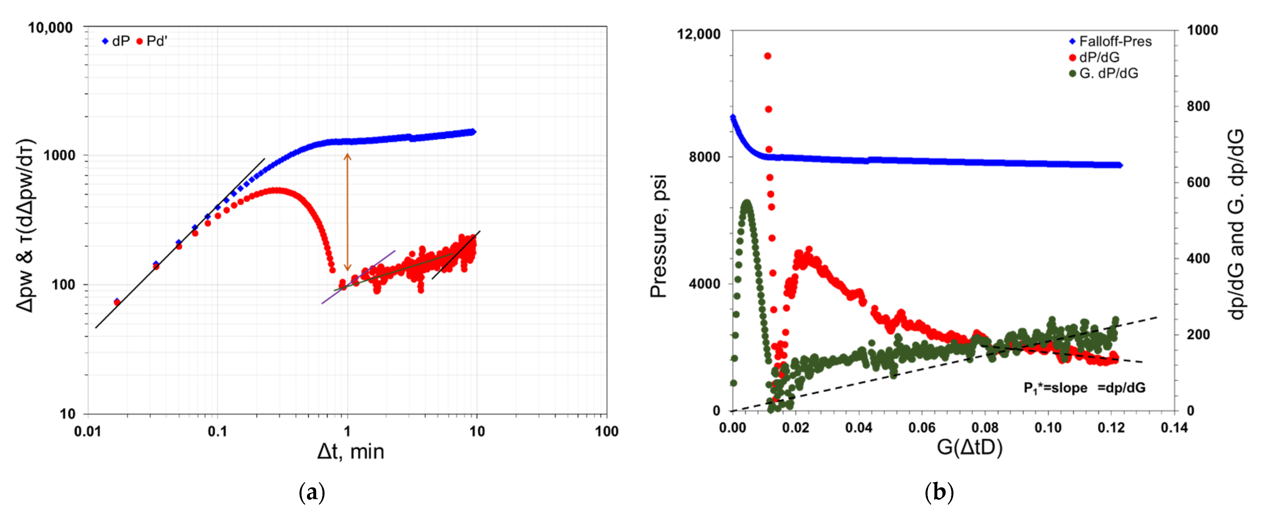
These assumptions may be realistic due to the characterization of the fracturing fluids and unconventional formations; therefore, Nolte’s technique may not work for unconventional formations and may yield overestimated results in parameters such as fluid efficiency, leak-off coefficient, and storage coefficient. This technique is a reliable application under some circumstances and is derived based on the G-function approach (Equation (2)). The pressure and G-function time are analyzed on log-log graphs to obtain the fracture closure point and other parameters, such as fluid efficiency and leak-off coefficient.

$$p_{ws}-p_w\left(\Delta t_D\right)=\frac{\pi r_p{C}_L\sqrt{t_p}}{2c_f}G\left(\Delta t_D\right)$$

(2)

$$p_1^{\ast }=\frac{\pi r_p{C}_L\sqrt{t_p}\left(A_{mf}+A_{nf}\right)}{2c_{mf}{A}_{mf}}$$

(3)

$$c_{mf}{A}_{mf}\left(ISIP-p_{c,mf}\right)=V_p-2r_p{C}_L\sqrt{t_p}\left(A_{mf}+A_{nf}\right)g_o$$

(4)

where, $p_{ws}$ is the pressure at the end of pumping, $p_w$ is the pressure recorded at the surface during the falloff period, and $\Delta t_D$ is the dimensionless time defined by:

$$\Delta t_D=\frac{t-t_p}{t_p}$$

(5)

$\tau$ is the superposition time defined by:

$$\tau =\frac{\Delta t+t_p}{\Delta t}$$

(6)

With pumping time $t_p$, falloff period $t$, productive fracture ratio $r_p=h/h_f$, fracture height $h_f$, propped height $h$, leak-off coefficient $C_L$, and fracture compliance $c_f$, $p_1^{\ast }$: $d{p}_w/dG$ at the closure point.

The pressure derivative equation is defined by:

$$\tau \frac{d\Delta p_w}{d\tau }=\left(\Delta t_D+\Delta t_D^2\right)\frac{d\Delta p_w}{d\Delta t_D}\tau \frac{d\Delta p_w}{d\tau }=\left(\Delta t_D+\Delta t_D^2\right)\frac{d\Delta p_w}{d\Delta t_D}$$

(7)

$$G\left(\Delta t_D\right)=\frac{4}{\pi }\left[g\left(\Delta t_D\right)-g_0\right]$$

(8)

where the g-function of time is approximated by:

$$g\left(\Delta t_D\right)=\left(1+\Delta t_D\right){\sin }^{-1}{\left(1+\Delta t_D\right)}^{-1/2}\alpha =1/2, \mathrm{low} \mathrm{fluid} \mathrm{efficiency}.$$

(9)

$$g\left(\Delta t_D\right)=\left(4/3\right)\left({\left(1+\Delta t_D\right)}^{3/2}-\Delta t_D{}^{3/2}\right)\alpha =1, \mathrm{high} \mathrm{fluid} \mathrm{efficiency}.$$

(10)

$g\left(\Delta t_D\right)$ is the loss-volume function, approximated analytically by Nolte (1979, 1986) [35,36] with the bounding values of the area exponent, $\alpha ,$ and $g_0$ is $g\left(\alpha ,\Delta t_D=0\right)$, see Table 2.

Castillo [37] later introduced a new G-function plot to address the assumption of pressure-dependent behavior by linearizing the relationship between the pressure falloff and time during the closure behavior. The relation is the time, such as the G-function time and the square root of time, on the X-axis vs. falloff pressure and the pressure derivative on the Y-axis. This approach reduces the uncertainty of estimating fracture fluid efficiency and the leak-off coefficient, while overestimated outcomes have resulted from Nolte’s method. The diagnostic plot estimates accurate pressure parameters, such as instantaneous shut-in pressure “ISIP,” closure pressure “Pc,” and Nolte match pressure “$p_1^{\ast }$”.

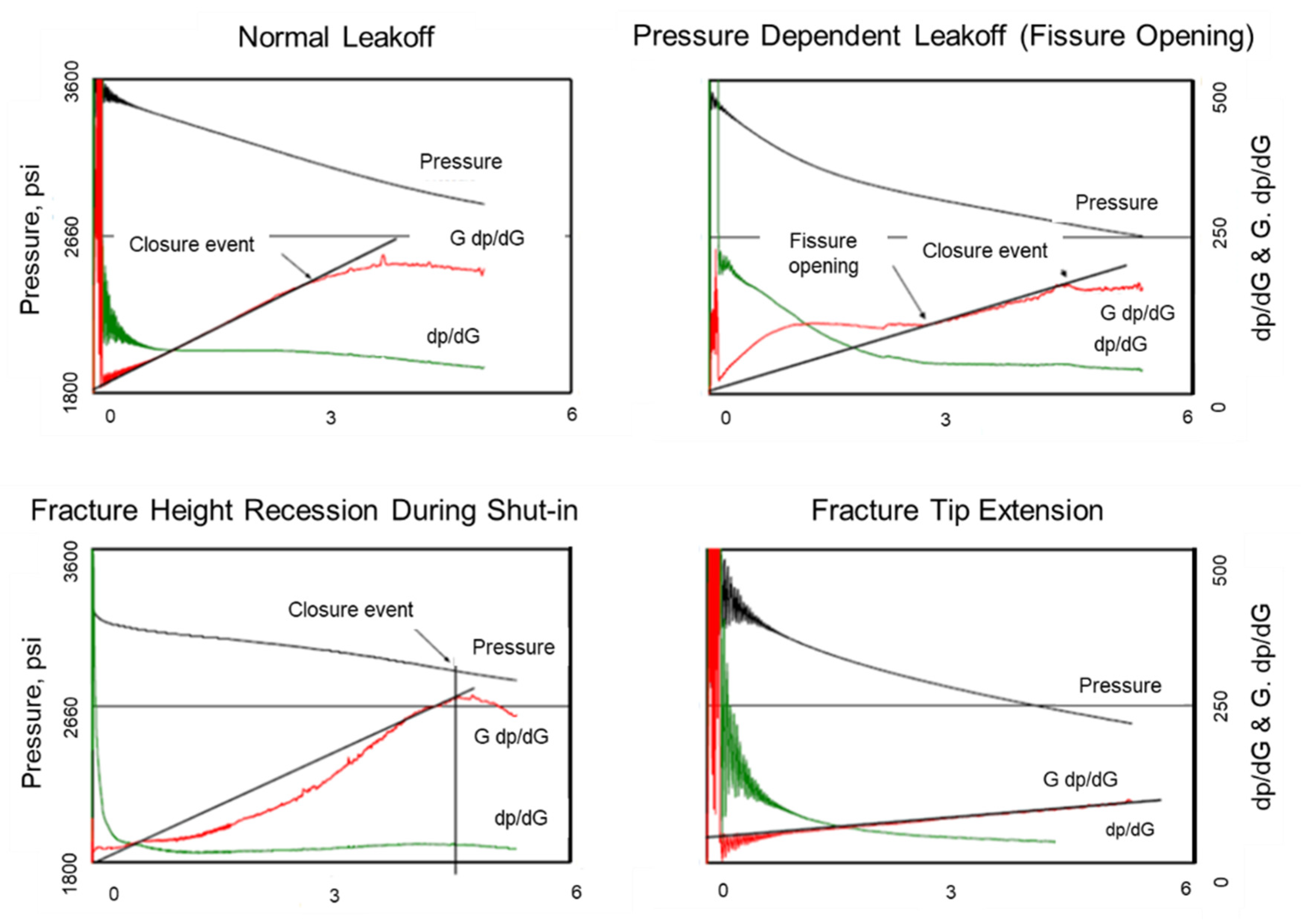
Barree and Mukherjee [38] presented several types of abnormal leak-off behaviors: (a) natural fracture opening or pressure-dependent leak-off, (b) fracture tip extension or recession, (c) height recession, (d) pressure-dependent fracture compliance, and (e) transient flow in the fracture. The authors developed Nolte’s work (1979, 1986) [35,36] for various closure behavior types and removed the ambiguity associated with understanding the complex fracture networks. The diagnostic plots allow us to predict an accurate estimation of the in-situ stress, fluid efficiency, leak-off coefficient, and pressure parameters. The G-function plot in the proposed models is the relationship between the following terms: falloff pressure, $p_w$, first pressure derivative, $d{p}_w/dG$, and second pressure derivative, $Gd{p}_w/dG$, on the Y-axis vs. the G-function time on the X-axis. The closure event is the point where the curve deviates from the straight line. Equations (11) through (13) are used to determine the primary outcomes, as listed in Table 3. This method enables us to identify the proper leak-off behavior for accurately estimating the hydraulic fracture geometries.

Table 3. Primary outcomes from a DFIT based on stipulated fracture geometry.

Results	Fracture Models			Equation
	PKN	KGD	Radial
$\mathrm{Fluid} \mathrm{efficiency}, \eta$	$\eta =\frac{G_c}{G_c+4g_0/\pi }$	$\eta =\frac{G_c}{G_c+4g_0/\pi }$	$\eta =\frac{G_c}{G_c+4g_0/\pi }$	(11)
$\mathrm{Fracture} \mathrm{dimensions}, x_f$$\mathrm{or} R_f$	$x_f=\frac{\left(1-\eta \right)V_{p}E\prime }{2{\beta }_s{g}_{0}p\ast }\left[\frac{1}{2h_f{}^2}\right]$	$x_f{}^2=\frac{\left(1-\eta \right)V_{p}E\prime }{2{\beta }_s{g}_{0}p\ast }\left[\frac{1}{4h_f}\right]$	$R_f{}^3=\frac{\left(1-\eta \right)V_{p}E\prime }{2{\beta }_s{g}_{0}p\ast }\left[\frac{3\pi }{32}\right]$	(12)
$\mathrm{Leak}-\mathrm{off} \mathrm{coefficient}, C_L$	$C_L=\frac{{\beta }_{s}p\ast }{r_p\sqrt{t_p}E\prime }\left[h_f\right]$	$C_L=\frac{{\beta }_{s}p\ast }{r_p\sqrt{t_p}E\prime }\left[2x_f\right]$	$C_L=\frac{{\beta }_{s}p\ast }{r_p\sqrt{t_p}E\prime }\left[\frac{32R_f}{3{\pi }^2}\right]$	(13)

Table 3. Primary outcomes from a DFIT based on stipulated fracture geometry.

Results	Fracture Models			Equation
	PKN	KGD	Radial
$\mathrm{Fluid} \mathrm{efficiency}, \eta$	$\eta =\frac{G_c}{G_c+4g_0/\pi }$	$\eta =\frac{G_c}{G_c+4g_0/\pi }$	$\eta =\frac{G_c}{G_c+4g_0/\pi }$	(11)
$\mathrm{Fracture} \mathrm{dimensions}, x_f$$\mathrm{or} R_f$	$x_f=\frac{\left(1-\eta \right)V_{p}E\prime }{2{\beta }_s{g}_{0}p\ast }\left[\frac{1}{2h_f{}^2}\right]$	$x_f{}^2=\frac{\left(1-\eta \right)V_{p}E\prime }{2{\beta }_s{g}_{0}p\ast }\left[\frac{1}{4h_f}\right]$	$R_f{}^3=\frac{\left(1-\eta \right)V_{p}E\prime }{2{\beta }_s{g}_{0}p\ast }\left[\frac{3\pi }{32}\right]$	(12)
$\mathrm{Leak}-\mathrm{off} \mathrm{coefficient}, C_L$	$C_L=\frac{{\beta }_{s}p\ast }{r_p\sqrt{t_p}E\prime }\left[h_f\right]$	$C_L=\frac{{\beta }_{s}p\ast }{r_p\sqrt{t_p}E\prime }\left[2x_f\right]$	$C_L=\frac{{\beta }_{s}p\ast }{r_p\sqrt{t_p}E\prime }\left[\frac{32R_f}{3{\pi }^2}\right]$	(13)

where, $G_c$, closure time, $E\prime$, Young’s modulus, $V_p$, total pumping volume, and ${\beta }_s$, the ratio of the average net pressure inside fractures to the maximum net pressure at the wellbore during the shut-in time (Table 2).

A DFIT uses the basis of conventional mini-fracture treatments that focus on acquiring treatment design parameters, such as fluid efficiency and leak-off behavior; however, this application is subtly different for unconventional formation analysis. This approach is used to acquire significantly more information on the created fractures and formation properties, such as pore pressure, closure and fracture gradients [11,20,28], process zone stresses [6], transmissibility values [39], leak-off mechanisms [6], natural fracture properties [6], fracture stiffness and un-propped fracture conductivity as a function of closure stress [20], and stimulation complexity and net pressure [40].

We can evaluate the properties of the main hydraulic fractures and natural fractures in a fracture treatment job by adopting the DFIT analysis method with no proppant. This method may not be ideal due to its tendency to ignore the impact of the proppant; however, it can be used with caution to evaluate post-treatment production and unconventional well performance.

4.3. DFIT Models: Before-Closure Analysis

Several analytical or semi-analytical models have been proposed for before-closure analysis (BC) [35,36,41,42,43], where all BC models were based on two fundamental concepts underlying the proposed methodology: (1) a material balance equation before fracture closure, and (2) the diffusive flow in the formation after closure. These models were founded based on two main conditions: (1) the total injection volume is equal to the sum of the fracture volume and cumulative leak-off volume, and (2) the fracture volume is estimated from the linear elasticity theory and a 2D fracture geometry during the pressure falloff period.

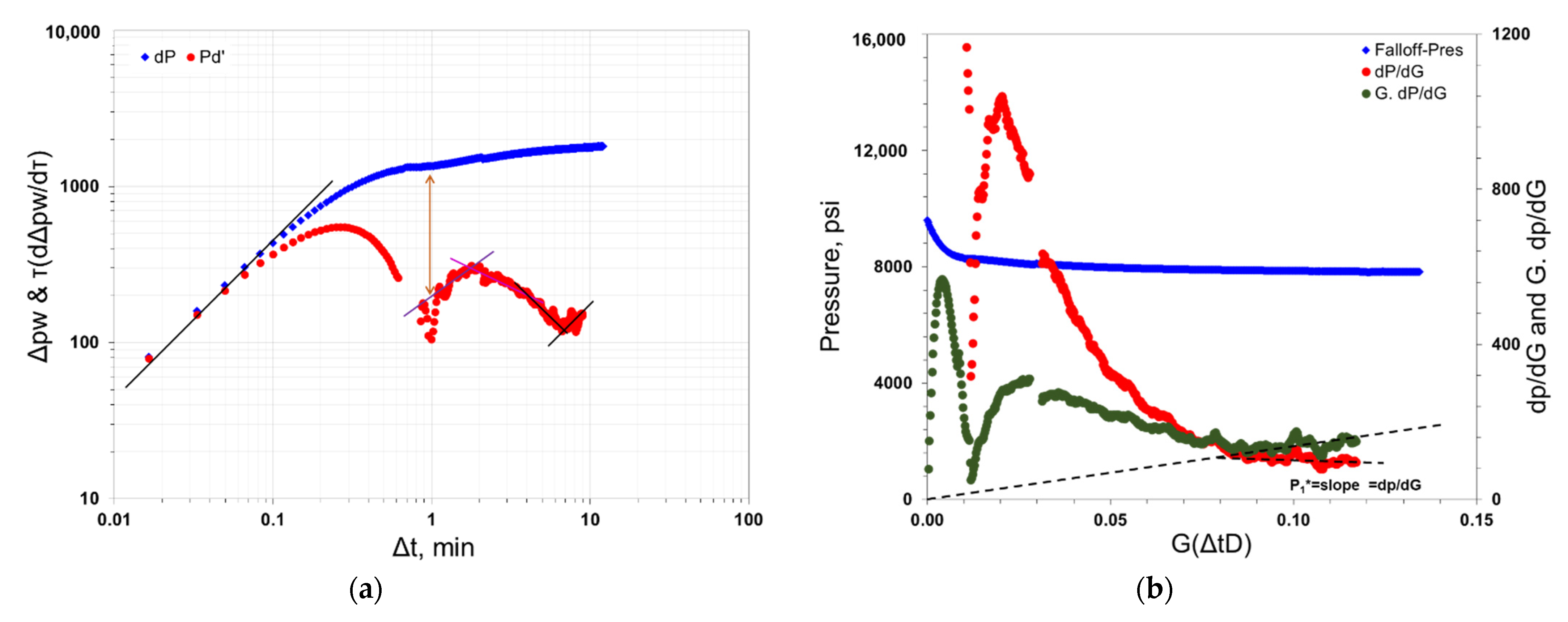
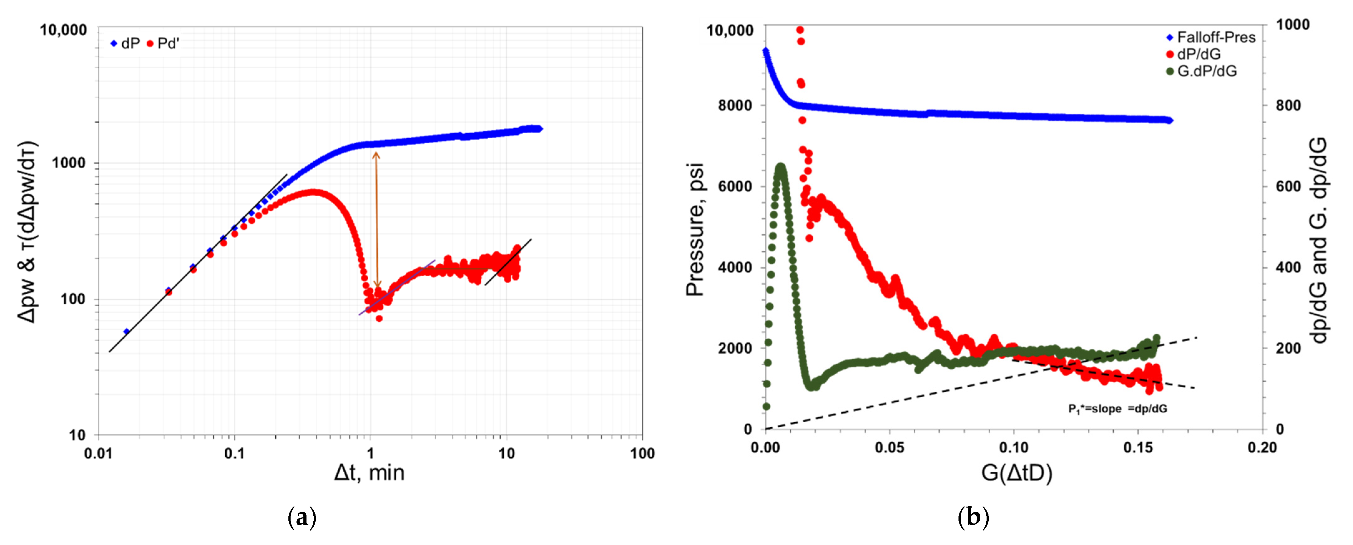
Cramer and Nguyen [44] reported that it would be rare to observe a normal leak-off behavior in the field, and closure behavior is commonly related to the abnormal leak-off concepts (Figure 5); therefore, the BC analysis must correctly address abnormal leak-off behaviors and near-wellbore friction losses. Liu and Ehlig-Economides [28] presented a model that was not limited to normal leak-off behavior compared to previous BC models [20,41,42,43]. These BC models relied on the assumptions of ideal leak-off behavior: (1) constant injection rate, (2) constant fracture surface area after shut-in, (3) creation of one main hydraulic fracture cluster without the effects of natural fractures, (4) constant fracture compliance during the operation, (5) assumption of similar fracture closure stresses for all stages, and (6) assumption that all injected fluid at the surface flows into the created fracture, meaning that the impact of the wellbore storage (WBS) is insignificant. Most current studies do not provide a quantitative discussion and do not address factors such as formation geology and mineralogy, resistance-dependent fluid distribution, and geomechanics parameters.

Table 4. Main results and methodologies of DFIT analysis.

Period	Results	Methods
Before closure	Total injection volume	Record time and rate.
Before closure	Fracture volume	Pressure falloff analysis by assuming linear elasticity and 2D fracture geometry (PKN and KGD models).
Before closure	Leak-off volume	Cater leak-off model. Diffusive linear flow from the fracture into the matrix.
After closure	Reservoir parameter	Conventional PTA.

summarizes DFIT analysis methods and the details of the fracture/reservoir property estimations from each period in a DFIT BC and AC.

Table 5. Definition of two main leak-off behaviors.

Type of Leak-Off Behavior	Definition
Normal leak-off behavior	Two scenarios can be considered for normal leak-off behavior: (a) All injected fluids leak-off through the fracture network. The fracturing fluid is accumulated and stored in the induced fractures, (b) All injected fluids leak-off across the contact surface area of the hydraulic fracture and are then recovered during flowback. The survey in this paper indicates that the assumptions mentioned above may not be appropriate for DFIT analysis in most field cases.
Abnormal leak-off behavior	In abnormal leak-off models, part of the injected fluids may leak-off into active secondary fractures. This behavior can be detected on the diagnostic plots from the following signature: (a) Higher stress on the diagnostic plot, compared to that of the main HF, may indicate the closure behavior of the secondary fracture network. The main hydraulic fracture propagates to the minimum principal stress.

lists the different leak-off models commonly used to analyze a DFIT, while

Table 6. DFIT’s outcomes from several field studies.

Type of Leak-Off Behavior	Duration	Results
Normal leak-off behavior	BC	Leak-off coefficient. Fluid efficiency. Fracture dimensions, such as fracture width and fracture half-length.
	AC	Permeability and skin. Reservoir pressure.
Abnormal leak-off behavior	BC	Friction losses in the wellbore. Perforation and near-wellbore tortuosity. Net pressure during and after shut-in. ISIP. Type of leak-off behavior and leak-off coefficient. Extension of secondary fractures. Tip extension distance after shut-in. Fracture surface area for natural fractures. Fracture geometry, such as fracture width and fracture half-length.
	AC	Permeability and skin. Reservoir pressure.

presents the outcomes from each model for several case studies. We have added our conclusions by summarizing the pros and cons of recently published models on abnormal leak-off behaviors (

Table 7. Recently published DFIT models under the conditions of abnormal leak-off behaviors.

Model	Pros	Cons
[41]	This type-curve method enables the analysis of the whole pressure falloff data, BC and AC, unlike previous methods (Nolte, 1979 [35]; Hagoort, 1981 [42]; Nolte, 1986 [36]) developed for only a specified portion of pressure falloff data, BC or AC.	The model does not account for fluid loss into natural fractures, such as diagnostic plots modeled based on normal leak-off behavior assumptions. The outcomes, such as the leak-off coefficient, fluid efficiency, and fracture surface area, are associated with high uncertainty.
[28]	This study investigated the effect of changing fracture compliance on pressure transience for unconventional formations, previously neglected during the closure behavior by previous research; therefore, the model provides accurate estimates of closure pressure analysis.	The standard models, such as PKN and KGD, simulate the created fractures; however, the actual fracture geometry is more complex due to the interaction between induced and fissure networks. Newtonian injection fluids and a fracture with uniform leak-off along the fracture face were assumed to form fracture geometry equations.
[9]	This model involves the impact of secondary fractures on fluids leak-off, where multiple closure events are observed on the G-function and Bourdet pressure derivative plots [46]. This approach reduces the need for a rate step-down test since this model allows us to perform a DFIT analysis to determine friction losses from near-wellbore tortuosity. This model can be used for the main fracture treatment design since it accounts for fluid leak-off into the natural and induced fractures.	The fluid efficiency estimated from the normal leak-off behavior is smaller than that of Nolte’s model. The model indicates inconsistency with other approaches. This work assumes that leak-off behaviors, such as closure behavior in secondary and created fractures, are governed by one constant leak-off coefficient for all apparent closure events. The surface fracture area calculations are associated with uncertainty due to ignoring the impact of the proppant. We recommend the inclusion of PIFs to estimate the effective contact areas to improve the DFIT assumptions.
[20]	This model accounts for fracture stiffness/compliance changes as the fracture closes; leak-off rate is a function of fracture pressure. This new concept promotes an understanding of pressure falloff and coupled behaviors during a DFIT with detailed support case studies.	This model assumes the closed fracture still retains fracture conductivity. Fluid leak-off remains constant through the fracture surface area before and after closure behavior.

).

We suggest developing the concept of DFIT to address this lack of a quantitative evaluation, allowing us to evaluate the post-treatment pressure falloff analysis in real-time fracture treatment job optimization. The accurate estimations of closure pressure, ISIP, and perforation and tortuosity friction losses can be obtained to prevent some far-field issues, such as well interventions, frac-hits, high apparent net pressure, and stress shadow. An effective evaluation of a stimulated formation before and during fracture treatment can identify optimal treatment design parameters for individual fracture stages.

4.4. Recommendations When Conducting and Interpreting DFIT

Table 8. Important points that extended in planning, executing, and achieving the successful DFIT.

Authors	Suggestions and Recommendations
	Field Execution	Data Analysis
[45]	The authors suggest injecting fracturing fluids at a low pumping rate for a short period to create a short fracture.	Reduce the time to reach fracture closure and AC pseudo linear and pseudo-radial flow.
[11]	The pumping rate for a DFIT should be set at a rate close to the planned rate, at least 75%, of the fracture treatment job. The same fracturing fluids should be used for both DFIT and fracture treatment operations. The range of the injection period should be between 3 to 5 minutes for a DFIT. The test should end by performing a rapid step-down test.	A successful DFIT design provides reliable closure identification and representative fracture and reservoir properties. A major assumption may not always be true.
[27]	The final execution relies on several factors, such as the design of the wellhead manifold, pressure gauge types and sampling time, stated objectives, time schedules, wellbore conditioning, pump rate, and pump volume. There are three surface located pressure gauges that should adhere to the specifications of 0.02% full-scale accuracy and 0.01 psi resolution. The test should be performed at the toe stage to fill the well with fracturing fluid. This process will activate pressure and bleeds back by circulating the treatment fluid until trapped gas bubbles are removed. Testing should be performed on the well casing, packers, tubing, and wellhead at high pressure. A diesel fluid should be injected on top of the wellbore water to avoid surface line and wellhead freezing.	Completion engineers may not over-tune or over-smooth the pressure Bourdet derivative when analyzing pressure falloff data since it can cause false flow regimes identification. Distinguishing between actual flow regime behavior and false look-alikes is critical. Reservoir engineers should link the fundamentals of fracture mechanisms with a physical response. The analysis of DFIT depends on the pressure accuracy; therefore, pressure sources can mitigate erroneous or uninterpretable DFIT pressure responses.

provides suggestions and recommendations that interpreters and operators should follow before any field execution or analysis to correctly perform a DFIT and achieve the research goals.

4.5. Lessons Learned from DFIT Operations

Table 9. Field case studies of DFIT operations and lessons learned.

Authors	Field/Country	Description	Results
[47]	Vaca Muerta Shale/Argentina	Two similar DFITs were performed in the same formation: (a) The first DFIT was performed with a small volume (20.8 bbl) and a low rate (≤5.5 bpm). (b) The second DFIT was designed with a large volume (155 bbl) and a high rate (≤14 bpm).	Diagnostic plots of both DFITs presented abnormal leak-off behaviors, but the difference in the closure signature was unexpected. (a) The diagnostic plots confirmed the transverse storage/height recession behavior for the first DFIT and the pressure-dependent leak-off (PDL) behavior for the second DFIT, (b) The final closure events were chosen using a holistic methodology, and the outcomes exhibited consistent values from both DFITs.
[48]	NIMR/Oman	Two successive informative field DFITs were reported, where they were performed in the same zone in a tight gas formation. (a) A small volume (24.8 bbl) at a low rate (0.94–1.38 bpm) was injected in the first DFIT, (b) The second DFIT was designed to pump a larger volume (158 bbl) at a higher pumping rate in the range of 12.6 to 18.7 bpm.	The results demonstrated a different fracture closure behavior. (a) The diagnostic plot of the first DFIT presented wellbore storage (WBS) followed by limited tip extension that defines a simple BC trend close to the behavior of normal leak-off, (b) The second DFIT illustrated a complicated BC behavior of variable fracture compliance under different categories that could be pressure-dependent leak-off (PDL), apparent height recession, or transverse storage, (c) The BC analysis was not consistent with the closure pressures quantified in both DFITs.
[49]	Eastern Alberta Shallow/Canada	The authors conducted the interpretation of two successive DFITs in a shallow gas-shale formation with a thrust fault setting. (a) The first injection had a relatively large volume, at 33.2 bbl, and a high rate at 6.3 bpm compared to the second injection, with an ultra-small volume of 0.82 bbl.	The results demonstrated a different fracture closure behavior. (a) The diagnostic plots of the first DFIT presented the behavior of transverse storage/height recession closure behavior, while the second DFIT illustrated a normal leak-off behavior, (b) The final closure chosen from those two DFITs was consistent but with different closure behavior types. The created fractures did not reopen due to a very small injection volume in the second DFIT.

provides lessons learned using a comparison study from DFIT field cases that have been reported in peer-reviewed journal articles. The objective is to explain the impact of operation conditions on DFIT interoperation and analysis of the outcomes.

4.6. How DFIT Analysis Is Applicable for Pressure Falloff Data of Main Fracture Treatments

Both DFIT and fracture treatment operations in unconventional horizontal wells have some similarities, especially in the created fractures and behavior of the pressure falloff data immediately after the treatment; however, several dissimilarities in the primary assumptions and operation conditions exist between the two techniques that must be addressed, examined, and basic formulae must be modified to obtain a representative analysis for pressure falloff behavior on a stage-by-stage basis in real-time. Very few studies [31] have analyzed pressure falloff data applications on a stage-by-stage basis in a horizontal wellbore. We have addressed the main differences between the two tests:

• A DFIT is performed by pumping a small volume (24.8 bbl) at a low rate (0.94–1.38 bpm), while the injection volume of the main fracture treatment in each stage is higher; therefore, the formation pore pressure may not be accounted for. We account for the formation pore pressure during the DFIT analysis.
• A DFIT only operates with water that does not include proppant, but the role of proppant exists in the main fracture treatment jobs. We recommend the inclusion of PIFs to improve the DFIT assumptions. We can apply the DFIT methodology to the main fracture treatment pressure falloff data to estimate an effective contact fracture surface area.
• A DFIT operation creates only one fracture, while hydraulic fracture treatments generate multiple perforation clusters in each stage. The fracture geometry is different from stage to stage on a well due to several factors, such as stress shadow effects, formation heterogeneity, formation lithology, and resistance-dependent fluid distribution.
• The falloff period immediately after DFIT is relatively long, up to a week compared to a short period of half an hour in the hydraulic fracture treatment, which is enough to perform the analysis.

4.7. Effective Fracture Surface Area Calculations

This section presents the workflow to analyze post-treatment pressure falloff data in order to estimate effective fracture surface areas for both natural fractures and hydraulic fractures on a stage-by-stage basis. Figure 6 illustrates our methodology, and

Table 10. Hydraulic fracture geometry calculations.

Fracture Half Length	Fracture Models	Equation
$x_f=\frac{V_{p}E\prime }{\pi {\beta }_s\left[ISIP-p_{c,mf}+4p_1^{\ast }{g}_o/\pi \right]}\left(\frac{1}{h_f^2}\right)$	PKN	(14)
$x_f=\sqrt{\frac{V_{p}E\prime }{\pi {\beta }_s\left[ISIP-p_{c,mf}+4p_1^{\ast }{g}_o/\pi \right]}\left(\frac{1}{2h_f}\right)}$	KGD	(15)
$R_f=\sqrt[3]{\frac{V_{p}E\prime }{\pi {\beta }_s\left[ISIP-p_{c,mf}+4p_1^{\ast }{g}_o/\pi \right]}\left(\frac{3\pi }{16}\right)}$	Radial	(16)
Effective Fracture Surface Area	Fracture Models	Equation
$A_{mf}=4x_f{h}_f$	PKN/KGD	(17)
$A_{mf}=\pi R_f^2$	Radial	(18)
$A_{nf}=A_{mf}\left[\frac{2c_{mf}{P}_1^{\ast }}{\pi r_p{C}_L\sqrt{t_p}}-1\right]$	PKN/KGD/Radial	(19)

lists the main Equations (14) through (19) that are used to determine the primary outcomes. The same concept was used to analyze the pressure falloff data by Liu et al. [9], who determined the total fracture surface area for both natural fractures and hydraulic fractures on a stage-by-stage basis. In this paper, we modified the workflow, which enables us to calculate fracture half-length and identify the main fracture flow regimes after the treatment of the Meramec Formation, STACK Play of the Anadarko Basin, Oklahoma.

5. Unconventional Well Case Study

5.1. Case Study Description

The DFIT was performed at the toe stage of an unconventional horizontal well (W2) in the Meramec Formation, STACK Play of the Anadarko Basin, Oklahoma. The STACK Play is a multi-layered tight oil reservoir “Meramec and Woodford Formations” with porosity lying in the range of 3% to 10%, and permeability in the range of 0.0001 to 0.01 mD. The plug and perf stimulation technique was used to complete the well. The wellbore was prepared before testing by filling it with fracturing fluids, typically water, to pressurize the top of the wellbore up to the point of completion so the formation did not break down if there were no pre-existing fractures. The fracturing fluid was pumped into the formation through the first casing interval with an inner diameter (ID) of 4.67 inches, a total vertical depth (TVD) of 9648 ft, and a measured depth (MD) of 19,635 ft. The pressure rises linearly with the injection volume during the injection period, while the injection rate remains constant (Figure 7). Figure 7 presents the injection and pressure profiles for our DFIT case study, where the surface injection rate was maintained at 12 bpm for approximately 40 min. The first shut-in period was measured for the same injection period, then the injection test was performed again with a higher injection rate of approximately 13 bpm. The test was then completed, and the pressure falloff data were recorded during the next 4–5 days.

The main fracture treatment job was performed in the same well (W2) based on the evaluation report from the DFIT analysis. Figure 8 presents the main hydraulic fracturing operation, where the job consists of several pump schedule stages, as shown in the figure by green and blue colors, and the slurry rates and proppant concentrations were changed during the operation. The total job period is around 160 min at an average 100 bpm slurry rate. At the end of the job, the falloff pressure was recorded for a period of time of approximately 15 min on average for all fracture stages. The fracture treatment strategy was applied with a constant pump schedule to create 36 frac stages, where each stage consisted of four to five clusters with 50 ft spacing.

This section presents a case study of the unconventional horizontal well, where

Table 11. Main hydraulic fracturing parameters and data quality check for post-treatment pressure analyses (W2).

Stage	Cluster Count	Pumping Time	Falloff Period	Pws	ISIP	TVD	Data Quality
(#)	(#)	(min)	(min)	(Psi)	(Psi)	(ft)	(-)
1	1	128	14	8112	7214	9676	Poor
2	5	171	15	7959	7629	9678	Poor
3	5	169	18	8465	7769	9682	Poor
10	5	168	17	8726	8117	9722	Poor
11	5	172	16	8179	7924	9732	Good
12	5	162	18	10,002	8047	9734	Good
13	5	166	30	9144	8055	9742	Good
14	5	166	17	9033	8146	9745	Poor
15	5	168	16	9147	8118	9755	Good
16	5	176	16	9399	8121	9766	Good
17	5	166	9	8954	8010	9766	Good
27	5	159	16	9405	8859	9818	Good
28	5	166	15	9685	8868	9821	Good
29	5	160	17	9146	8740	9830	Good
30	5	158	17	9530	8676	9834	Good
31	5	159	17	9697	8554	9829	Good
32	5	159	19	8943	8575	9836	Good
35	5	156	13	9322	8002	9903	Good
36	5	153	18	9907	8559	9923	Good
Max		176	20	10,186	9399	9923
Min		128	9	7985	7214	9676
Avg		162	17	9092	8210	9779

shows the main fracture treatment operation parameters as well as preprocessing data quality for each fracture stage. The combination of DFIT and pressure falloff data immediately after the treatment was used to identify fracture and reservoir behavior characteristics to assess the evaluation of the fracture stages.

5.2. Results of Case Study including DFIT and Main Fracture Treatment Analysis

Figure 9 and Figure 10 illustrate the analysis of the DFIT test using two diagnostic plots: (1) a Bourdet pressure derivative plot [46] (Figure 9), and (2) the plot of the G-function diagnostic analysis (Figure 10). Both plots indicate consistent results and the same height recession leak-off behavior. The mechanisms of this closure fracture behavior are defined as most of the fracturing fluid’s leak-offs into neighboring layers, a common behavior for unconventional formations. The plots also indicate that natural fractures have contributed to the multiple fracture closure events observed before the closure analysis.

Different trends, such as circle 1, appear to be wellbore storage coupled with friction dissipation. The following flat trend, circle 2, appears to be tip extension with limited growth distance, as shown in Figure 11. Linear flow with ½ signature, circle 3, is indicated on the plot before the closure behavior, marked by the green dashed line. Two closure events overlay on a 3/2 slope, circle 4, that depicts the closure behavior of the natural and induced fractures. The reservoir dominated flow observed after the closure analysis with two flow regimes started by linear flow, a ½ slope, circle 5, was followed by radial flow, and a zero slope, circle 6, where formation permeability can be estimated. The main results from DFIT analysis are listed in

Table 12. Summary of the main DFIT outcomes of the Meramec Formation for W2.

Flow Regime Behaviors	Slopes	Pressure, psi	Time, min	Permeability, md
WBS	1
Tip extension	0
Linear flow	½
Fracture closure (Fissures)	1.5	6944	31.5
Fracture closure (HF)	1.5	6125	210
Linear flow	½
Radial flow	0
Pi =		4521
k =				0.0038
P*1 =		48
P*2 =		79
ISIP =		7535

, where the formation is classified with low permeability in the range of 0.004 md and closure pressure in 6100 psi.

The same concept was used to analyze the pressure falloff data by Liu et al. [9], who determined the total fracture surface area for both natural fractures and hydraulic fractures on a stage-by-stage basis. However, we modified the workflow to improve the data quality, minimizing the effects of water hammers for the first 2 min in falloff pressure data and including the analysis of the G-function plot in order to validate fracture flow regimes, as well as considering variable parameters for each stage. This methodology has not been applied before in the literature, and it is more precise with low uncertainty compared to previous research, where constant values were used for all stages to estimate total fracture surface areas. Our case study shows three different behaviors after the main fracture treatment as follows:

• Case #1, ¼ slope, tip extension of the main fracture: Figure 12 presents the behavior of tip extension of the main hydraulic fracture, where the results showed that the fracture surface area for the main fracture is higher than the total fracture surface area for the natural fracture. The reason is that low total pressure losses and more fracturing fluids leak-off through main fractures instead of nearby neighbor layers.
• Case #2, –1/2 and –1 slope, fracture height recession: Figure 13 shows the behavior of fracture height recession, where the results confirmed the DFIT signature for the Meramec formation. The reason is that more fracturing fluids are leaking off through nearby neighbor layers instead of creating a longer fracture half-length.
• Case #3, 0 slope, open fissures. Figure 14 illustrates the behavior of open fissures, where the treatment created a high natural fracture surface area compared to the main hydraulic fracturing area as a result of communications with neighbor stages. The reason is that the treatment generated higher total pressure losses compared to two previous cases with shorter fracture half-length since all fracturing fluids leaked off through natural fracture. Additionally, this behavior indicates frac-hit phenomena due to interaction and communication between child and parent wells.

For more detailed results,

Table 13. Outcomes of pressure falloff analyses for the main hydraulic fracture treatment of W2.

Stage	Δpwb&per	Δptort	Δptotal fric	Pc,nf	Pc,mf	ISIP	${\mathit{p}}_1^{\ast }$	Amf	Anf
(#)	(Psi)	(Psi)	(Psi)	(Psi)	(Psi)	(Psi)	(Psi)	(ft2)	(ft2)
11	944	340	1283	7778	7530	7891	1789	225,162	392,586
13	948	318	1266	8002	7780	8091	1704	231,059	380,939
15	598	244	842	7964	7676	8051	1247	230,521	325,202
32	451	261	712	8226	8044	8575	568	274,479	33,713
35	704	287	991	8207	7786	8321	1574	74,499	161,706
36	1022	419	1441	8620	8012	8818	1400	115,360	214,029

provides the analysis outcomes, including friction pressure losses and total fracture surface area.

6. Past, Present, and Future Research Directions

Very few studies [9] have investigated the pressure falloff behavior combined with DFIT analysis to evaluate the effectiveness of fracture treatment conditions stage-by-stage; however, the assessment of fracture design quality stage-by-stage must still be studied, especially after treatment. The principle of DFIT needs to be adjusted by counting PIFs to estimate the effective fracture contact area, or the propped fracture area per unit length of lateral, which is one key factor for evaluating post-treatment performance. An integral approach using several diagnostics tools is necessary to develop the technology for determining the contribution of individual fracturing treatments when multiple factors are considered. This approach can be accomplished using a series of neural network models to predict fracture geometry, fracture directions, number of clusters needed, proppant loading, fracture complexity, and treatment costs during fracture treatment. A data-driven model must be created to apply an integral approach in real-time, a challenge that must be addressed with thorough discussion, especially given the lack of literature on this subject. These combination methods involve machine learning tools that can assist us in understanding fracture treatment effectiveness, assess new completion technologies, and evaluate which formations are the most productive. This technology is feasible for real-time analysis to apply an optimum pump schedule for the current and next treatment stages on a well.

7. Summary

In this study, we employed an integral approach to identify fracture and reservoir behavior characteristics to assess the performance of hydraulic fractures stage-by-stage. The research findings highlight the following:

• Diagnostic tools have become attractive to the oil and gas industry since they are powerful methods for identifying fracture and reservoir characteristics. The analysis of these approaches is based on data type, which guides the assessment of complex fracture networks generated by hydraulic fracture treatment operations.
• The use of falloff pressure data is a simple approach since it does not require more information than shut-in pressure vs. time. The data are recorded immediately after shut-in at no additional cost; however, micro-seismic monitoring is expensive, and the production data analysis has high uncertainty.
• The models proposed by Liu and Ehlig-Economides [28] allowed us to perform DFIT analysis to determine flow friction losses in the wellbore, perforation, and near-wellbore tortuosity separately without the need for rate step-down tests. These models are the primary means by which we can calculate the total fracture surface area for the secondary fractures and hydraulic fractures and gain insight into the effectiveness of the hydraulic fracturing process.
• Barree et al. [11] and Liu and Ehlig-Economides [28] reported that their data supported a holistic methodology that allows them to pick the hydraulic fracture closure, which contradicts the variable fracture compliance approach from McClure et al. [50].
• Rizwan [48] created an alternative methodology to apply a DFIT, where a change in the test operation strategy may cause a change in fracture closure behavior. This study provided insight into expected fracture closure behavior during the main fracture treatment.
• We concluded that evaluating the performance of post-stimulation conditions on a stage-by-stage basis using indirect methods, such as pressure falloff data analysis, is the most promising technique for providing a wide range of information covering the mechanics of the hydraulic fracture, such as open, closed, and propped. This method may overcome limitations and weaknesses found in many of the proposed techniques reported in peer-reviewed journal articles, such as production data analysis and micro-seismic methods.
• This technology is a critical factor in the economic development of unconventional reservoirs since the well completion cost is a significant portion of the capital cost compared to other expenses, and heavily influences production rate or ultimate recovery.
• We suggest combining static and dynamic diagnostic methods to better estimate fracture geometry through pressure data, diagnostic fracture injection tests (DFIT), micro-seismic fracture mapping, distributed temperature sensing (DTS), production logs, and production data. The full suite of information can provide valuable evidence concerning the details of the treatment and well performance from complicated shale plays.
• Three different cases were observed through diagnostic plots, where mainly the analysis indicates that most of the fracturing fluid was leaked off through the natural fracture surface area and resulted in the estimation of larger values compared to the hydraulic fracture calculated area. These phenomena might represent a secondary fracture set with a high fracture closure stress activated in neighbor stages that was not well-developed in other sections.
• This conclusion fits with our discussion that provided detailed information with support case studies to apply the technology of post-treatment pressure analysis in real-time.

References

1. Abbasi, M.A.; Ezulike, D.O.; Dehghanpour, H.; Hawkes, R.V. A comparative study of flowback rate and pressure transient behavior in multifractured horizontal wells completed in tight gas and oil reservoirs. J. Nat. Gas Sci. Eng. 2014, 17, 82–93. [Google Scholar] [CrossRef]
2. He, J.; Lin, C.; Li, X.; Wan, X. Experimental investigation of crack extension patterns in hydraulic fracturing with shale, sandstone and granite cores. Energies 2016, 9, 1018. [Google Scholar] [CrossRef] [Green Version]
3. Ellafi, A.; Jabbari, H. Understanding the mechanisms of huff-n-puff, CO2-EOR in liquid-rich shale plays: Bakken case study. In Proceedings of the SPE Canada Unconventional Resources Conference, Calgary, AL, Canada, 18–19 March 2020. [Google Scholar] [CrossRef]
4. Jayaram, V.; Hull, R.; Wagner, J.; Zhang, S. Hydraulic fracturing stimulation monitoring with distributed fiber optic sensing and microseismic in the Permian Wolfcamp shale play. In Proceedings of the SPE/AAPG/SEG Unconventional Resources Technology Conference 2019, Denver, CO, USA, 22–24 July 2019. [Google Scholar] [CrossRef]
5. Parvizi, H.; Gomari, S.R.; Nabhani, F.; Monfared, A.D. Modeling the risk of commercial failure for hydraulic fracturing projects due to reservoir heterogeneity. Energies 2018, 11, 218. [Google Scholar] [CrossRef] [Green Version]
6. Li, K.; Gao, Y.; Lyu, Y.; Wang, M. New mathematical models for calculating proppant embedment and fracture conductivity. SPE J. 2015, 20, 496–507. [Google Scholar] [CrossRef]
7. Qin, Q.; Xue, Q.; Ma, Z.; Zheng, Y.; Zhai, H. Hydraulic fracturing simulations with real-time evolution of physical parameters. Energies 2021, 14, 1678. [Google Scholar] [CrossRef]
8. Nguyen, T.; Pande, S.; Bui, D.; Al-Safran, E.; Nguyen, H. Pressure dependent permeability: Unconventional approach on well performance. J. Pet. Sci. Eng. 2020, 193, 107358. [Google Scholar] [CrossRef]
9. Liu, G.; Zhou, T.; Li, F.; Li, Y.; Ehlig-Economides, C.A. Fracture surface area estimation from hydraulic-fracture treatment pressure falloff data. SPE Drill. Complet. 2020, 35, 438–451. [Google Scholar] [CrossRef]
10. EIA. Annual Energy Outlook 2019 with Projections to 2050; US Department of Energy: Washington, DC, USA, 2019. Available online: https://www.eia.gov/out-looks/aeo (accessed on 20 November 2019).
11. Barree, R.D.; Miskimins, J.L.; Gilbert, J.V. diagnostic fracture injection tests: Common mistakes, misfires, and misdiagnoses. SPE Prod. Oper. 2014, 30, 84–98. [Google Scholar] [CrossRef]
12. Alfarge, D.; Wei, M.; Bai, B. Evaluating the performance of hydraulic-fractures in unconventional reservoirs using production data: Comprehensive review. J. Nat. Gas Sci. Eng. 2018, 61, 133–141. [Google Scholar] [CrossRef]
13. Cipolla, C.L.; Wright, C. Diagnostic techniques to understand hydraulic fracturing: What? Why? and How? SPE Prod. Facil. 2002, 17, 23–35. [Google Scholar] [CrossRef]
14. Economides, M.J.; Ehlig-Economides, C.A.; Tosic, S. Application of pressure-transient and production-data analysis for hydraulic-fracture-treatment evaluation. In Proceedings of the SPE Hydraulic Fracturing Technology Conference 2007, College Station, TX, USA, 29–31 January 2007. [Google Scholar]
15. Haskett, W.J.; Brown, P.J. Evaluation of unconventional resource plays. In Proceedings of the SPE Annual Technical Conference and Exhibition 2005, Dallas, TX, USA, 9–12 October 2005. [Google Scholar]
16. Daniels, J.L.; Waters, G.A.; Le Calvez, J.H.; Bentley, D.; Lassek, J.T. Contacting more of the Barnett shale through an integration of real-time microseismic monitoring, petrophysics, and hydraulic fracture design. In Proceedings of the SPE Annual Technical Conference and Exhibition 2007, Anaheim, CA, USA, 11–14 November 2007. [Google Scholar]
17. Evans, K.F.; Kohl, T.; Rybach, L.; Hopkirk, R.J. The effects of fracture normal compliance on the long-term circulation behavior of a hot dry rock reservoir: A parameter study using the new fully coupled code “fracture”. Geotherm. Resour. Counc. Trans. 1992, 16, 449–456. [Google Scholar]
18. Fu, C.; Liu, N. Waterless fluids in hydraulic fracturing—A review. J. Nat. Gas Sci. Eng. 2019, 67, 214–224. [Google Scholar] [CrossRef]
19. Guo, T.; Zhang, S.; Qu, Z.; Zhou, T.; Xiao, Y.; Gao, J. Experimental study of hydraulic fracturing for shale by stimulated reservoir volume. Fuel 2014, 128, 373–380. [Google Scholar] [CrossRef]
20. Wang, H.; Sharma, M.M. A novel approach for estimating formation permeability and revisiting after-closure analysis of diagnostic fracture-injection tests. SPE J. 2019, 24, 1809–1829. [Google Scholar] [CrossRef]
21. Gonzalez, M.; Taleghani, A.D.; Olson, J.E. A cohesive model for modeling hydraulic fractures in naturally fractured formations. In Proceedings of the SPE Hydraulic Fracturing Technology Conference 2015, The Woodlands, TX, USA, 3–5 February 2015. [Google Scholar]
22. Wright, C.A.; Weijers, L.; Germani, G.A.; MacIvor, K.H.; Wilson, M.K.; Whitman, B.A. Fracture treatment design and evaluation in the Pakenham field: A real-data approach. In Proceedings of the SPE Annual Technical Conference and Exhibition 1996, Denver, CO, USA, 6–9 October 1996. [Google Scholar] [CrossRef]
23. Jabbari, H.; Zeng, Z. Hydraulic fracturing design for horizontal wells in the Bakken formation. In Proceedings of the 46th US Rock Mechanics/Geomechanics Symposium 2012, Chicago, IL, USA, 24–27 June 2012. [Google Scholar]
24. Kurtoglu, B.; Salman, A.; Kazemi, H. Production forecasting using flow back data. In Proceedings of the SPE Middle East Unconventional Resources Conference and Exhibition 2015, Muscat, Oman, 26–28 January 2015. [Google Scholar] [CrossRef]
25. Ilk, D.; Okouma, V.; Blasingame, T.A. Characterization of well performance in unconventional reservoirs using production data diagnostics. In Proceedings of the SPE Annual Technical Conference and Exhibition 2011, Denver, CO, USA, 30 October–2 November 2011. [Google Scholar] [CrossRef] [Green Version]
26. Witherspoon, P.A. Development of underground research laboratories for radioactive waste isolation. In Proceedings of the Second International Symposium on Dynamics of Fluids in Fractured Rock, Berkeley, CA, USA, 10–12 February 2004; pp. 3–7. [Google Scholar]
27. Hawkes, R.V.; Bachman, R.; Nicholson, K.; Cramer, D.D.; Chipperfield, S.T. Good tests cost money, bad tests cost more—A critical review of DFIT and analysis gone wrong. In Proceedings of the SPE International Hydraulic Fracturing Technology Conference and Exhibition, Muscat, Oman, 16–18 October 2018. [Google Scholar] [CrossRef]
28. Liu, G.; Ehlig-Economides, C. Comprehensive before-closure model and analysis for fracture calibration injection falloff test. J. Pet. Sci. Eng. 2018, 172, 911–933. [Google Scholar] [CrossRef]
29. Warpinski, N.; Branagan, P.; Engler, B.; Wilmer, R.; Wolhart, S. Evaluation of a downhole tiltmeter array for monitoring hydraulic fractures. Int. J. Rock Mech. Min. Sci. 1997, 34, 329.e1–329.e13. [Google Scholar] [CrossRef]
30. Ezulike, O.; Dehghanpour, H.; Virues, C.; Hawkes, R.V.; Jones, R.S. Flowback fracture closure: A key factor for estimating effective pore volume. SPE Reserv. Eval. Eng. 2016, 19, 567–582. [Google Scholar] [CrossRef]
31. Xu, Y.; Ezulike, O.D.; Zolfaghari, A.; Dehghanpour, H.; Virues, C. Complementary surveillance microseismic and flowback data analysis: An approach to evaluate complex fracture networks. In Proceedings of the SPE Annual Technical Conference and Exhibition 2016, Dubai, United Arab Emirates, 26–28 September 2016. [Google Scholar] [CrossRef]
32. Fisher, M.; Heinze, J.; Harris, C.; Davidson, B.; Wright, C.; Dunn, K. Optimizing horizontal completion techniques in the Barnett shale using microseismic fracture mapping. In Proceedings of the SPE Annual Technical Conference and Exhibition 2004, Houston, TX, USA, 26–29 September 2004. [Google Scholar]
33. Maxwell, S.; Urbancic, T.; Demerling, C.; Prince, M. Real-time 4D passive seismic imaging of hydraulic fracturing. In Proceedings of the SPE/ISRM Rock Mechanics Conference 2002, Irving, TX, USA, 20–23 October 2002. [Google Scholar] [CrossRef]
34. Warpinski, N.R.; Mayerhofer, M.J.; Agarwal, K.; Du, J. Hydraulic-fracture geomechanics and microseismic-source mechanisms. SPE J. 2013, 18, 766–780. [Google Scholar] [CrossRef]
35. Nolte, K. A general analysis of fracturing pressure decline with application to three models. SPE Form. Eval. 1986, 1, 571–583. [Google Scholar] [CrossRef]
36. Nolte, K.G. Determination of fracture parameters from fracturing pressure decline. In Proceedings of the SPE Annual Technical Conference and Exhibition 1979, Las Vegas, NV, USA, 23–26 September 1979. [Google Scholar] [CrossRef]
37. Castillo, J. Modified fracture pressure decline analysis including pressure-dependent leakoff. In Proceedings of the SPE/DOE Joint Symposium on Low Permeability Reservoirs 1987, Denver, CO, USA, 18–19 May1987. [Google Scholar] [CrossRef]
38. Barree, R.; Mukherjee, H. Determination of pressure dependent leak off and its effect on fracture geometry. In Proceedings of the SPE Annual Technical Conference and Exhibition 1996, Denver, CO, USA, 6–9 October 1996. [Google Scholar] [CrossRef]
39. Soliman, M.Y.; Miranda, C.G.; Wang, H.M. Application of after-closure analysis to a dual-porosity formation, to CBM, and to a fractured horizontal well. SPE Prod. Oper. 2010, 25, 472–483. [Google Scholar] [CrossRef]
40. Potocki, D.J. Understanding induced fracture complexity in different geological settings using DFIT net fracture pressure. In Proceedings of the SPE Canadian Unconventional Resources Conference 2012, Calgary, AL, Canada, 30 October–1 November 2012. [Google Scholar] [CrossRef]
41. Craig, D.P.; Blasingame, T.A. Application of a new fracture-injection/falloff model accounting for propagating, dilated, and closing hydraulic fractures. In Proceedings of the SPE Gas Technology Symposium 2006, Calgary, AB, Canada, 15–17 May 2006. [Google Scholar]
42. Hagoort, J. Waterflood-Induced Hydraulic Fracturing. Ph.D. Thesis, Delft University, Delf, The Netherlands, 1981. [Google Scholar]
43. Mayerhofer, M.; Economides, M. Permeability estimation from fracture calibration treatments. In Proceedings of the SPE Western Regional Meeting 1993, Anchorage, Alaska, 26–28 May 1993. [Google Scholar] [CrossRef]
44. Cramer, D.D.; Nguyen, D.H. Diagnostic fracture injection testing tactics in unconventional reservoirs. In Proceedings of the SPE Hydraulic Fracturing Technology Conference 2013, The Woodlands, TX, USA, 4–6 February 2013. [Google Scholar]
45. Marongiu-Porcu, M.; Retnanto, A.; Economides, M.J.; Ehlig-Economides, C. Comprehensive fracture calibration test design. In Proceedings of the PE Middle East Unconventional Resources Conference and Exhibition 2015, Muscat, Oman, 4–6 February 2015. [Google Scholar] [CrossRef]
46. Bourdet, D.; Ayoub, J.A.; Pirard, Y.M. Use of pressure derivative in well test interpretation. SPE Form. Eval. 1989, 4, 293–302. [Google Scholar] [CrossRef] [Green Version]
47. Rohmer, B.; Raverta, M.; de la Combe, J.-L.B.; Jaffrezic, V. Minifrac analysis using well test technique as applied to the Vaca Muerta shale play. In Proceedings of the EUROPEC 2015, Madrid, Spain, 1–4 June 2015. [Google Scholar] [CrossRef]
48. Rizwan, Y. Pressure Transient Analysis for Minifracs/DFIT and waterflood induced fractures. Master’s Thesis, The Delft University of Technology, Delf, The Netherlands, 2017. [Google Scholar]
49. Nicholson, A.K.; Bachman, R.C.; Hawkes, R.V. How diagnostic fracture injection tests (DFITs) show horizontal plane tensile and shear fractures in various stress settings. In Proceedings of the SPE/AAPG/SEG Unconventional Resources Technology Conference 2017, Austin, TX, USA, 24–26 July 2017. [Google Scholar] [CrossRef]
50. McClure, M.W.; Blyton, C.A.J.; Jung, H.; Sharma, M.M. The effect of changing fracture compliance on pressure transient behavior during diagnostic fracture injection tests. In Proceedings of the SPE Annual Technical Conference and Exhibition 2014, Amsterdam, The Netherlands, 27–29 October 2014. [Google Scholar] [CrossRef]
Figure 1. Average oil production per well in the Bakken Formation, Williston Basin, North Dakota [10].
Energies 14 06747 g001
Figure 2. Typical pressure behavior includes a sequence of main events observed in a DFIT. ISIP is instantaneous shut-in pressure.
Energies 14 06747 g002
Figure 3. Typical flow regimes before and after closure behaviors.
Energies 14 06747 g003
Figure 4. Observation of fracture closure behavior.
Energies 14 06747 g004
Figure 5. G-function characteristics for different leak-off mechanisms [41].
Energies 14 06747 g005
Figure 6. Workflow of research methodology to determine fracture stage performance.
Energies 14 06747 g006
Figure 7. DFIT operations for W2, presenting injection and pressure profiles.
Energies 14 06747 g007
Figure 8. Main hydraulic fracturing operations for W2, presenting injection, pressure, proppant concentration profiles, and micro-seismic events.
Energies 14 06747 g008
Figure 9. DFIT analysis and Bourdet pressure derivative plots for W2.
Energies 14 06747 g009
Figure 10. DFIT analysis and G-function plots for W2.
Energies 14 06747 g010
Figure 11. DFIT analysis, observation of open fissures’ behavior through G-function plot for W2.
Energies 14 06747 g011
Figure 12. (a) Case #1, Bourdet pressure derivative plots for the main hydraulic fracture treatment for W2. (b) Case #1, G-function plots for the main hydraulic fracture treatment for W2.
Energies 14 06747 g012
Figure 13. (a) Case #2, Bourdet pressure derivative plots for the main hydraulic fracture treatment for W2. (b) Case #2, G-function plots for the main hydraulic fracture treatment for W2.
Energies 14 06747 g013
Figure 14. (a) Case #3, Bourdet pressure derivative plots for the main hydraulic fracture treatment for W2. (b) Case #3, G-function plots for the main hydraulic fracture treatment for W2.
Energies 14 06747 g014