Abstract
Anaerobic digestion processes offer the possibility for wastewater treatment while obtaining a benefit through the obtained biogas. This paper aims to continue the effort to adopt data-driven control methods in the case of anaerobic digestion processes. The paper proposes a data-based Internal Model Control approach applied to an anaerobic digestion process. The paper deals extensively with the issue of choosing the reference model and proposing an engineering approach to this issue. The paper also addresses the issue of verifying robust stability, a very important aspect considering the uncertainties that characterize bioprocesses in general. The approach proposed in the paper is validated through a numerical simulation using the Anaerobic Digestion Model No. 1. During the validation of the proposed control solution, the main operating conditions were analyzed, such as the setpoint tracking performance, the rejection of disturbance generated by variations in the influent concentration, and the effect of the measurement noise on the controlled variable.
1. Introduction
The problem of treating the wastewater resulting from human and industrial activities is a key aspect in the sustainable development of society [1,2]. In the case of urban wastewater, aerobic treatment technologies with activated sludge are preferred [3]. They also include an anaerobic digestion unit used in processing the activated sludge excess coming from the aerobic treatment units. However, in this case, the control of the anaerobic digester is minimal, and only needs to ensure some optimal conditions for the process (e.g., temperature) [4]. In the case of industries that discharge water with a high biological load, or of isolated human areas, it is preferable to use anaerobic digestion technologies that have the advantage of being able to treat wastewater with high biological load, while benefiting economically from the advantage of producing biogas, which is a renewable energy source. In this case, the control problem is much more complex, addressing the issue of modeling, implementation of software estimators and control itself, as evidenced by the large number of papers in the literature.
Modeling the anaerobic digestion process has been done by two approaches. The first approach is to obtain as detailed a model as possible, which makes a complex description of the physical, chemical and biological phenomena that take place. Undoubtedly the model considered the most evolved in this case is Anaerobic Digestion Model No. 1 (ADM1) [5]. However, the complexity of this model, with 35 state variables, makes it very difficult to use in control problems. Consequently, there has been a continuous effort to obtain simplified models that allow the application of methods to obtain software solutions for estimating the state variables and parameters of interest, and for implementing control solutions. In the mathematical mode proposed in [6] a model with 6 state variables is proposed. In [7] a modified variant of the simplified model is proposed with a generic procedure to obtain the model from the complex model ADM1. More recent approaches [8] propose inclusion of hydrogen evolution in a simplified model.
Different control strategies and methodologies were used to increase the efficiency of the process. Starting from the simplified model, a linearizing feedback control was applied together with an asymptotic observer and interval observer software estimator solution [9]. In fact, the linearizing control solution has often been used in anaerobic digestion processed [10,11]. A robust quantitative feedback theory control solution is implemented in the context of using an optimal reference in [12], and a modern control solution is based on the model-free control method in [13]. Another intensely used solution is Extremum Seeking Control used both in a deterministic context and in a stochastic approach [14], either using the external dither signal [15] or a solution that takes advantage of the usual variability of the existing influence in wastewater [16]. An exhaustive presentation of estimation and control techniques is made in [17]. A newer approach is to use data-driven methods, such as Virtual Reference Feedback Tuning [18], which allow them to be designed using the complex ADM1 model. In fact, this is also the context of the present paper in which the Data-Driven IMC method is used [19].
Internal Model Control (IMC), introduced in 1982 [20], is currently one of the most widespread control structures used in process engineering [21,22,23]. IMC has grown due to its simple mechanism and intuitive design. Consequently, the adoption of the IMC structure to control the ADP is a solution of real interest. The implementation of the IMC is a real challenge in calculating the inverse of the transfer function matrix of the ADP, because its model is complex and has a large dimension. The data-driven controller design in the IMC structure is a problem in the literature [24,25,26,27] in the context of designing control laws for various processes, such as chemical reactors and activated sludge process.
The main contribution of this paper is the analysis of the context for the application of the data-driven IMC method in the case of anaerobic digestion processes. Thus, an important aspect is the choice of the reference model. This model must be chosen considering the following aspects: essential information on the desired dynamics for the closed-loop process; the level of dynamic errors resulting in a closed loop for the adopted reference model, and the maximum amplitude of the disturbance that would cause a major deterioration of control quality. Based on the results obtained, the issue of design of the control structure and the verification of robust stability is treated taking into account the uncertainties that characterize bioprocesses in general. Finally, the underlined practical aspects are validated considering a “virtual plant” constituted by the complex model ADM1 in which the essential problems were considered, i.e., the setpoint tracking performance, the rejection of disturbance represented by the influent concentration, and the effect of measurement noise on the controlled variable.
2. Materials and Methods
2.1. The Anaerobic Digestion Process
The anaerobic digester (AD) used in the case study presented in this paper has a volume of liquid and a volume of gas . The digester is considered well-mixed and the temperature in the digester is controlled at an optimal value. The ADM1 model, which has 35 state variables, was implemented in accordance with [28]. The objective of the control problem is to track the chemical oxygen demand (COD) concentration at a setpoint compatible with environmental norms. This is defined by the relation , where is the sum of the concentrations of the organic substrate components, and is the sum of the volatile fatty acid concentrations [7]. The command variable is the dilution rate (or the influent flow rate in AD, ), and the disturbance variables are the concentration variations in the influent, and .
2.2. The Principle of the Data-Driven IMC Approach
A graphical representation of the IMC structure is shown in Figure 1 together with the corresponding notations. The nonlinear ADP model of the ADM1 type is not explicitly used in the design of the controller, but only through the input-output data it provides. The objective is to achieve a setpoint-output transfer () in accordance with the required reference model, , and also to achieve reduced effect of the disturbance, , on the output, . We consider as the transfer function of the linearized model at the current operating point, obtained by ideal linearization, with the remark that is not known.
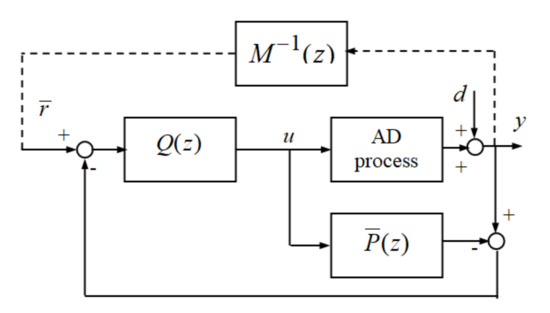
Figure 1.
ADP control using the IMC structure: reference model, —process linear model included in the IMC controller, —controller.
The control structure contains the controller itself, with the ideal transfer function , as well as the internal linear model of the process, . If then the setpoint is ideally transmitted at the output, in open loop, if . One can see that such a controller is not causal.
If a reference model, , is adopted so that the transfer function:
is invertible (i.e., to represent a system at the casual limit), then:
where is the discrete time, and notation of the form signifies the transfer through the system.
The control structure uses , as is unknown and, moreover, does not ideally reflect the properties of the nonlinear process. However, from the analysis of the idealized model of the system (see Equation (1)) it results that the controller has the function of compensating the dynamics of the process, so that the transfer is determined by the reference model .
Let be a controller that performs this function at a level of performance imposed by the design procedure. In this case, by analogy with Equation (1), valid in the hypothesis of idealized models, an approximation of is deduced. Let be this approximation, which is a component of the IMC control structure:
Therefore, if the reference model is chosen and there is a computation procedure for the transfer function , then the Equation (3) allows the computation of the second block in the IMC structure. In order to obtain the transfer function , first the reference is determined as a result of the transfer of through the inverted reference model:
and this reference is applied to the input of the controller. If, for the controller, a linear structure in the parameters are adopted, meaning an FIR system with the transfer function , then computation of the parameter vector is achieved by minimizing the criterion:
using the least squares method.
In conclusion, the data-based design of the controller uses the data and the collected in open loop operation of the ADP at a given operating point, as well as the “reference” computed with Equation (4), after choosing a reference model. Therefore, the optimal parameters obtained by minimizing the criterion given by Equation (5) are not affected by the colored noise . This noise is transmitted on the feedback pathway in closed loop operation when the controller input is , where is the setpoint of the IMC system.
A key issue in the data-driven design of the IMC structure is to ensure robust stability. This requirement is due to uncertainties in the adoption of the model in the control structure. It is considered that, when choosing the model, the upper limit of the multiplicative uncertainties expressed in the frequency domain, is :
If, in a closed loop system, the adopted model deviates from the real model without exceeding the limit given by Equation (6), then the system is robustly stable. The condition for the closed loop system to be robustly stable, given in [29] and also in [26,30] is:
3. Results and Discussion
3.1. The Choice of the Reference Model
The choice of the reference model was made based only on the input-output data available for the synthesis of the controller. Through this model the desired performances of the closed loop were imposed. The choice of is a key issue in the design of the control structure, as it determines the specifical expressions of the and transfer functions, as well as ensuring the robust stability. Checking the loop performances by simulation and particularly the robust stability analysis may lead to iterations in the synthesis of the control structure which would also lead to the correction of the reference model chosen initially.
The reference model must lay between two limits:
- (1)
- An invertible broadband model, the highest frequency of which is limited by the Shannon frequency required for data sampling. In this case, determining the ”reference” by the transfer function (see Equation (4)) leads to the use of a broadband derivative system, eventually multiple derivatives. By minimizing the criterion given in Equation (5), a controller, , with derivative components is obtained, defined in an excessive frequency band, which is inadequate since: (a) there are limitations to the variations of the command variable (derivations lead to large amplitude variations which are not physically achievable); (b) the noise is excessively amplified and (c) robust stability may be compromised;
- (2)
- An invertible low frequency model, at the limit, can be a static amplification theoretically equal to the inverse of the static amplification of the process: . In this case it is expected that the dynamic performance of the closed loop system is very modest.
The reference model must be between the two limits mentioned above. In an engineering approach, it is necessary to search for the starting from the modest dynamic performances imposed to the closed loop system (i.e., starting from an invertible low frequency model) then successively increasing the dynamic performance imposed by until obtaining a controller, , with a moderate dynamic component of the PD type. The specification “moderate dynamic component of PD type” applied to the block means the lack of higher order derivative components and the existence of a frequency band of about 1–1.5 decades in which the derivative component manifests. However, when physically implementing the IMC control, adjustment iterations of the controller are possible by adjusting the , in order to decrease/increase this frequency bandwidth. Within these iterations, the is determined for the current reference model and then the frequency properties of the obtained controller are analyzed.
Consideration was given to a process operating regime around the static operating point given by and . The input-output data are depicted in Figure 2.
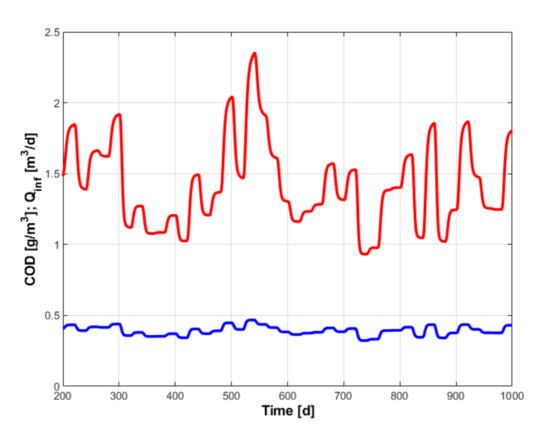
Figure 2.
Input (blue) and output (red) data collected by process simulation using the ADM1 model.
The transfer function of the used reference model is [31]:
where is the order of the model, is the parameter that determines the width of its frequency band, and is the sampling period. As the parameter increases, the duration of the dynamic regime of the reference model decreases.
The inverse model is:
The design of the IMC controller is based on the input-output data from the open loop operation of the process. To comment on some results of the command synthesis procedure, a linearized model of the process is used. This model is obtained by identification using the available input-output data without involving this model in the synthesis procedure. Figure 3 shows the variations from the average values of the output variables of the process and of the identified model. The identification was done using the least squares method and considering a fourth order linear model. The modest quality of the identification by least squares method is due to important nonlinearities of the process model, but the identified model allows the formulation of qualitative comments on the procedure for choosing the reference model.
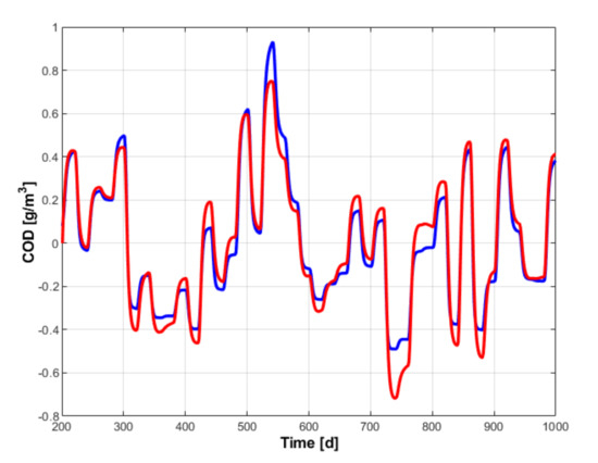
Figure 3.
Variations from the average values of the process output sizes (blue) and the identified pattern (red).
In the reference model given by Equation (6) is adopted, which ensures a dynamic without an overshoot. The choice of the parameter , which determines the settling time, is made based on prior information on the process dynamics. “Candidate” values are adopted: , which are tested in the following procedure.
- (1)
- A qualitative analysis of the step responses of the model is performed in relation to the dynamics reflected by the process data, but also with respect to the information from engineering practice regarding the response time of the closed-loop process. It is also useful to examinate the Bode plot of the inverse model to assess the bandwidth available to compensate the process dynamics. The candidate values adopted for in what follows are: . Figure 4 shows the step responses of the considered reference models and of the identified process model. The latter’s response illustrates the complexity of the process: the initial rapid variation is determined by hydraulic and biochemical processes, while the slow variation lasting up to days is determined by microbiological processes. A Bode plot of the inverted reference models, shown in Figure 5, highlights large frequency domains, with a double derivative character, which would create insurmountable difficulties for the problem of transfer through the of a noisy signal from the physical process. In the case of the control design procedure based on the data from the simulated process, there is practically no noise and the data transfer through the inverted model is done without problems.
- (2)
- Determine the fictitious reference by transferring the signal through .
- (3)
- Based on the data the linear model is identified:

Figure 4.
The process response for a step of amplitude 0.1 () and the unit step responses of reference models with .

Figure 5.
Bode plot of reference models with .
For example, for and , the identified parameters are represented in Figure 6.
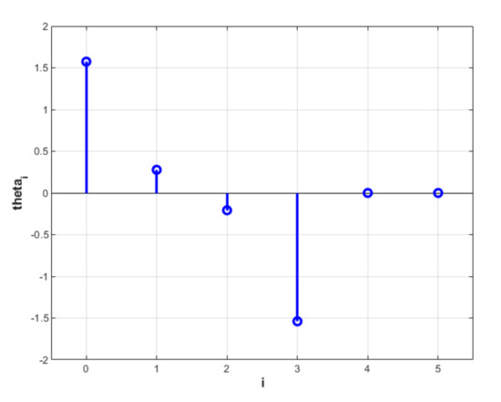
Figure 6.
Controller parameters for and .
- (4)
- The graphical representation of the frequency characteristics of is made, for all “candidate” values of the parameter of the reference model, considering in each case for the order of the controller. Thus, the representations given in Figure 7, Figure 8 and Figure 9 are obtained, which are made on the same scale to facilitate their comparative analysis.
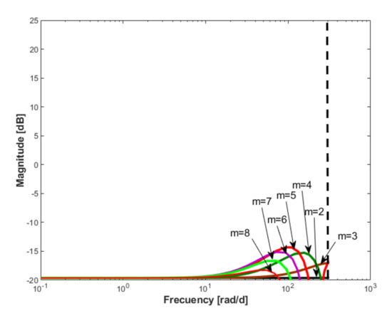 Figure 7. The Bode characteristics of the for and .
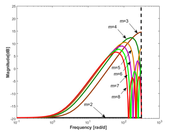 Figure 8. The Bode characteristics of the for and .
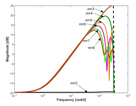 Figure 9. The Bode characteristics of the for and .
The resulting findings, presented below, are important not only for the selection of the reference model, but also for the choice of the preliminary form of the controller. Regarding the choice of the reference model, it is useful to correlate the obtained Bode characteristics of the controller with the responses of the given in Figure 4. The main findings are:
- For , the resulting Bode characteristics indicate a negligible dynamic, which manifests itself only in an area adjacent to the Shannon frequency. In this case, the controller is practically a constant, equal to the inverse of the process gain. The controller does not effectively perform a compensation function of the process dynamics and we can conclude that the choice of the reference model is not a satisfactory solution.
- If the order of is , the controller is basically a static gain equal to the inverse of the process gain, regardless of the value of the parameter.
- The excessive increase of the order of the controller is not appropriate, as it leads to a reduction of the frequency bandwidth with derivative effect. For and , the Bode characteristics are practically overlaid until near to the Shannon frequency.
- For , the Bode characteristics of the controller manage to compensate the dynamic characteristic of the process starting from a frequency that can be considered excessively low and are able to ensure a derivative behavior of the controller in a frequency band of more than two decades. Even if a filter is introduced in the final design phase of the controller in the area adjacent to the Shannon frequency, the solution seems debatable from the point of view of feasibility. This finding correlates with the response depicted in Figure 4, which indicates a closed loop system response time of about one day, which is an overly optimistic performance.
- The choice , for , seems to be an appropriate solution, because a compensation of the process dynamics is performed without performing this compensation in an excessive frequency bandwidth. Correlating the time response of the closed loop system of about 2–3 days reinforces this conclusion.
3.2. Design of the Control Structure
For better transparency of the correlation between the controller parameters with the parameters of the reference model, the digital-analog conversion of the transfer functions involved in the analysis of the control structure was performed.
The transfer function of the reference model for is:
After the identification of the model for , and reducing the order of the equivalent analog model, we obtain:
Figure 10 shows the Bode plot of the analog controller given in Equation (9) compared to that of the identified controller. In the same picture there is depicted the Bode characteristic obtained for the discretized controller given in Equation (9). Here, the frequency band with derivative effect extends over approximatively two decades, which leads to excessive noise amplification. In order to impose an extended derivative effect in a frequency band of approximatively one decade, the time constant is adopted at the denominator of the transfer function given in Equation (9), instead of . Under these conditions, the transfer function, obtained with Equation (3) and implemented in the control structure is:
It is known that the IMC structure implements a control law corresponding to a classical regulator with the transfer function:

Figure 10.
The Bode plot for: identified (red), low order analog (brown), low order digital (blue) and limited frequency digital (green).
The Bode characteristic of type PID of this controller is shown in Figure 11.
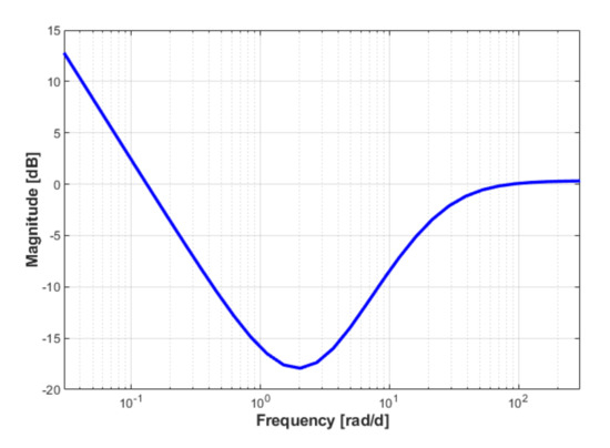
Figure 11.
The Bode characteristics of the controller achieved through the IMC control structure.
3.3. Checking Robust Stability
Checking the condition given by Equation (7) requires the assessment of the upper boundary of the multiplier uncertainties. Since the only available information on the controlled process are the input-output data , obtaining the transfer function based on these data and on the transfer functions from the control structure is done using the Empirical Transfer Function Estimate (ETFE) method, introduced in [32] and also used in [25,30]. Let us consider the general case of a system with transfer function, in which the discrete values of the input-output variables are known: , and, respectively, . In the above-mentioned papers, the estimate of the frequency response of the system is defined by:
where:
The discrete frequency values in the frequency response are: .
In [32], it is shown that such a computation procedure leads to an ETFE asymptotically unbiased with the increase of , but the ETFE variance does not decrease with the increase of . So, the presented procedure leads to a result affected by strong numerical noise, so that the use of a smoothing operation, adapted to the concrete application, is required.
Imposing in Equation (7) the condition, the closed loop system is robustly stable if:
In practice a security parameter is adopted, which is necessary given that is calculated as an estimate, so the existence of uncertainties justifies this approach. Let be this security parameter. In this case, the robust stability condition is:
The operations required for the effective verification of robust stability are included in the following algorithm, proposed in [25,30]:
Initial data: , , , , .
- Compute: ;
- Compute: ;
- Compute defined by as output and as input, using ETFE;
- Compute defined by as output and as input, using ETFE;
- Compute: ;
- For each the condition is checked.
The initial data, used to check the robust stability, came from the set, represented in Figure 1, which served to synthesize the command law. These data were extracted using the sampling period , resulting in samples. Obviously, this number is prohibitive in the ETFE calculation procedure. Consequently, a new data set with samples was extracted from the initial data, with the sampling period . Figure 12 shows a zoom of the data set which includes the signals and with the sampling period , represented in blue and red dashed line, respectively, as well as the impulses from those signals extracted with the sampling period.
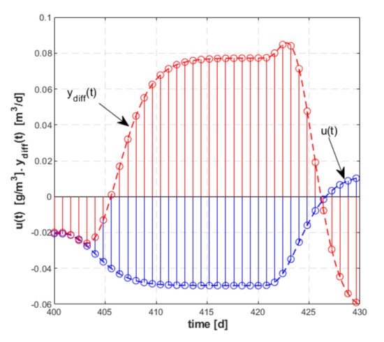
Figure 12.
The and signals with the sampling period (blue and red dashed line, respectively) and the impulses from these signals extracted with the sampling period.
Adopting , the robust stability condition given by Equation (19) is checked based on the representation in Figure 13 of the functions and .
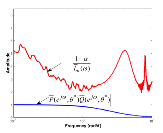
Figure 13.
Checking the robust stability of the system.
3.4. Validation by Simulation of the Designed Control Structure
Analysis by numerical simulation of the performances of the synthesized control law follows three aspects: (1) following the setpoint ; (2) the rejection of the disturbance and (3) the effect of the measurement noise on the controlled variable.
- (1)
- The setpoint tracking performances are illustrated in Figure 14a,b. The delay of the controlled variable with respect to the setpoint, when it has a variation close to a ramp, is less than one day, and the maximum error during the dynamic regime is ;
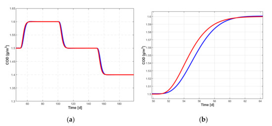 Figure 14. Setpoint tracking: setpoint (red), controlled variable ( —blue) (a); zoom (b).
 - (2)
- The rejection of disturbance was examined in relation to the variation of the influent concentration () presented in Figure 15. The evolution of the controlled variable, , and of the setpoint, , are shown in Figure 16. A performance evaluation must also be made considering the evolution of the command variable, , shown in Figure 17. Its variations around the stationary value related to the current operating regime, , are small enough, so that it can be appreciated that the hypothesis of linearizing the mathematical model of the process is valid. We can test and determine the maximum amplitude of the disturbance that would cause a major deterioration of the control quality. Thus, if the amplitude of the disturbance is doubled, then the results presented in Figure 16 and Figure 17 become those in Figure 18a,b, respectively. This shows that the quality of the control is not significantly affected, and the variation of the operating point in dynamic regime covers the interval where the nonlinearities are already significant.
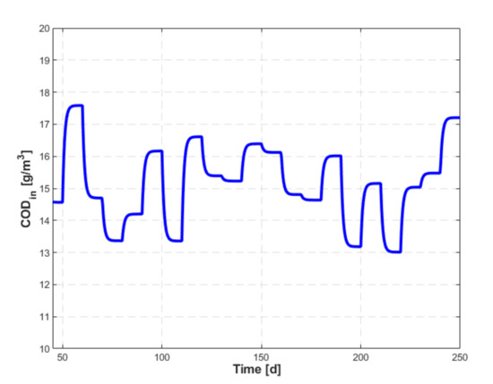 Figure 15. Evolution of the influent .
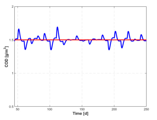 Figure 16. Evolution of the setpoint (red) and the controlled variable (blue).
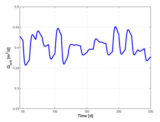 Figure 17. Command variable evolution.
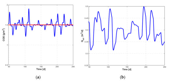 Figure 18. (a) The set point (red) and the controlled variable (blue); the command variable (b).
The presented results may suggest the testing of the designed command law around a more efficient reference model. If is adopted in Equation (8), the following transfer functions are obtained:
and
In this case the delay of the controlled variable in relation to the reference is reduced (see Figure 19). If the amplitude of the disturbance amplitude increases four-fold in relation to the regime illustrated in Figure 15, then the evolution of the controlled variable and the command variable are presented in Figure 20a,b, respectively, together with the evolution of the same variables (see Figure 16 and Figure 17) from the situation considered as reference. It is found that the dynamic errors are important, and the variations of the command variable in dynamic regime extend in the region of nonlinear variation from the static characteristics , without the system losing its stability.
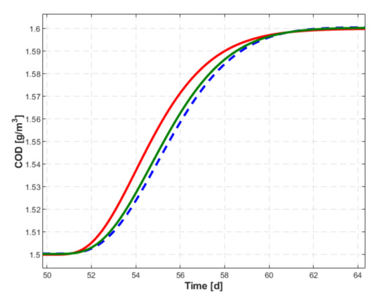
Figure 19.
Evolution of the controlled variable for (green) in relation to the set point (red). For the controlled variable is represented with dashed blue line.
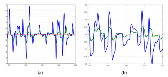
Figure 21 shows the functions and , for and . It is found that by adopting the new reference, decrease in the stability margin is insignificant.
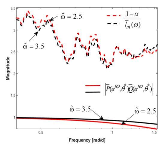
Figure 21.
Analysis of the robust stability margin for and .
- (3)
- The effect of a measurement noise with the standard deviation on the controlled variable was tested. Under these conditions, the standard deviation of the controlled variable is , and the evolution of this variable is given in Figure 22.
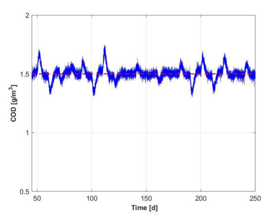 Figure 22. Effect of measurement noise on the controlled variable.
4. Conclusions
The key findings of this paper are:
- The IMC approach results in an extremely attractive solution for the data-based design of the control law for ADP. However, the adoption of these methods requires taking into consideration the specificity of these processes.
- Due to the nonlinearities of the process, the command law must be based on the gain scheduling strategy, and the design of the local regulators based on a procedure that, according to the results presented, ensures a good reserve of robust stability.
- An essential step of the data-based design procedure of the control law in the IMC structure is the choice of the reference model, which is involved in the calculation of the transfer functions and . Usually, the reference model is established following iterations of adjustment of the control structure. The main data used to select the reference model are the essential information on the dynamics of the closed-loop process, the level of dynamic errors resulting in a closed loop for the adopted reference model, the maximum amplitude of the disturbance that would cause a major deterioration of the regulator quality, and robust stability reserve.
Our future work will focus on obtaining a control solution based on the gain scheduling method, and validating this on an anaerobic digester.
Author Contributions
Authors contributed equally to this paper. All authors have read and agreed to the published version of the manuscript.
Funding
The work of Larisa Condrachi is supported by the project “ANTREPRENORDOC”, in the framework of Human Resources Development Operational Programme 2014–2020, financed from the European Social Fund under the contract number 36355/23.05.2019 HRD OP/380/6/13 – SMIS Code: 123847. Ramón Vilanova acknowledges the support of the Catalan Government under Project 2017 SGR 1202 and of the Spanish Government through the MICINN project PID2019-105434RB-C33.
Institutional Review Board Statement
Not applicable.
Informed Consent Statement
Not applicable.
Acknowledgments
The authors dedicate this paper to the memory of Emil Ceangă who was the initiator of the research on data-driven control at “Dunărea de Jos” University of Galaţi.
Conflicts of Interest
The authors declare no conflict of interest.
References
- Barbu, M.; Vilanova, R.; Meneses, M.; Santin, I. On the evaluation of the global impact of control strategies applied to wastewater treatment plants. J. Clean. Prod. 2017, 149, 396–405. [Google Scholar] [CrossRef]
- Barbu, M.; Santin, I.; Vilanova, R. Applying Control Actions for Water Line and Sludge Line to Increase Wastewater Treat-ment Plant Performance. Ind. Eng. Chem. Res. 2018, 57, 5630–5638. [Google Scholar] [CrossRef]
- Santin, I.; Barbu, M.; Pedret, C.; Vilanova, R. Control strategies for nitrous oxide emissions reduction on wastewater treat-ment plants operation. Water Res. 2017, 125, 466–477. [Google Scholar] [CrossRef] [PubMed]
- Revollar, S.; Meneses, M.; Vilanova, R.; Vega, P.; Francisco, M. Eco-Efficiency Assessment of Control Actions in Wastewater Treatment Plants. Water 2021, 13, 612. [Google Scholar] [CrossRef]
- Batstone, D.J.; Keller, J.; Angelidaki, I.; Kalyuzhnyi, S.V.; Pavlostathis, S.G.; Rozzi, A.; Vavilin, V.A. The IWA anaero-bic digestion model No 1 (ADM1). Water Sci. Technol. 2002, 45, 65–73. [Google Scholar] [CrossRef]
- Bernard, O.; Hadj-Sadok, Z.; Dochain, D.; Genovesi, A.; Steyer, J.-P. Dynamical model development and parameter identification for an anaerobic wastewater treatment process. Biotechnol. Bioeng. 2001, 75, 424–438. [Google Scholar] [CrossRef]
- Hassam, S.; Ficara, E.; Leva, A.; Harmand, J. A generic and systematic pro-cedure to derive a simplified model from the An-aerobic Digestion Model No. 1(ADM1). Biochem. Eng. J. 2015, 99, 193–203. [Google Scholar] [CrossRef]
- Giovannini, G.; Sbarciog, M.; Steyer, J.-P.; Chamy, R.; Wouwer, A.V. On the derivation of a simple dynamic model of anaer-obic digestion including the evolution of hydrogen. Water Res. 2018, 134, 209–225. [Google Scholar] [CrossRef]
- Petre, E.; Selişteanu, D.; Şendrescu, D. Adaptive and robust-adaptive control strategies for anaerobic wastewater treatment bioprocesses. Chem. Eng. J. 2013, 217, 363–378. [Google Scholar] [CrossRef]
- Petre, E.; Selisteanu, D.; Sendrescu, D.; Barbu, M.; Caraman, S. An adaptive control structure for an anaerobic digestion process with unknown inputs. In Proceedings of the 2017 18th International Carpathian Control Conference (ICCC), Sinaia, Romania, 28–31 May 2017; pp. 58–63. [Google Scholar]
- Simeonov, I.; Queinnec, I. Linearizing control of the anaerobic digestion with addition of acetate (control of the anaerobic digestion). Control. Eng. Pr. 2006, 14, 799–810. [Google Scholar] [CrossRef]
- Condrachi, L.; Ceanga, E.; Georgescu, L.P.; Murariu, G.; Vilanova, R.; Barbu, M. Model-based optimization of an an-aerobic digestion process. In Proceedings of the 2018 22nd International Conference on System Theory, Control and Computing, ICSTCC 2018, Sinaia, Romania, 10–12 October 2018. [Google Scholar]
- Condrachi, L.; Vilanova, R.; Ceanga, E.; Barbu, M. The Tuning of a Model-Free Controller for an Anaerobic Digestion Process using ADM1 as Virtual Plant. IFAC-Pap. 2019, 52, 99–104. [Google Scholar] [CrossRef]
- Caraman, S.; Barbu, M.; Ifrim, G.; Titica, M.; Ceanga, E. Anaerobic Digester Optimization Using Extremum Seeking and Model-Based Algorithms. A Comparative Study. IFAC-Pap. 2017, 50, 12673–12678. [Google Scholar] [CrossRef]
- Caraman, S.; Ifrim, G.; Ceanga, E.; Barbu, M.; Titica, M.; Precup, R.-E. Extremum seeking control for an anaerobic digestion process. In Proceedings of the 2015 19th International Conference on System Theory, Control and Computing (ICSTCC), Cheile Grădiştei, Romania, 14–16 October 2015; pp. 243–248. [Google Scholar]
- Barbu, M.; Ceangă, E.; Vilanova, R.; Caraman, S.; Ifrim, G. Extremum-Seeking Control Approach Based on the Influent Variability for Anaerobic Digestion Optimization. IFAC-Pap. 2017, 50, 12623–12628. [Google Scholar] [CrossRef]
- Jimenez, J.; Latrille, E.; Harmand, J.; Robles, Á.; Ferrer, J.; Gaida, D.; Wolf, C.; Mairet, F.; Bernard, O.; Alcaraz-Gonzalez, V.; et al. Instrumentation and control of anaerobic digestion processes: A review and some research challenges. Rev. Environ. Sci. Bio/Technol. 2015, 14, 615–648. [Google Scholar] [CrossRef]
- Condrachi, L.; Ceanga, E.; Vilanova, R.; Bichescu, C.; Barbu, M. The Anaerobic Digestion Process Control Using Data Driven Methods. In Proceedings of the 2019 23rd International Conference on System Theory, Control and Computing (ICSTCC), Sinaia, Romania, 9–10 October 2019; IEEE: Piscataway, NJ, USA, 2019; Volume 14, pp. 242–248. [Google Scholar]
- Condrachi, L.; Vilanova, R.; Barbu, M. Data-Driven Internal Model Control of an Anaerobic Digestion Process. In Proceedings of the 25th International Conference on System Theory, Control and Computing (ICSTCC), Iaşi, Romania, 20–23 October 2021. [Google Scholar]
- Garcia, C.E.; Morari, M. Internal model control. A unifying review and some new results. Ind. Eng. Chem. Process. Des. Dev. 1982, 21, 308–323. [Google Scholar] [CrossRef]
- Morari, M. Internal Model Control—Theory and Applications. IFAC Proc. Vol. 1983, 16, 1–18. [Google Scholar] [CrossRef]
- Rivera, D.E.; Morari, M.; Skogestad, S. Internal model control: PID controller design. Ind. Eng. Chem. Process. Des. Dev. 1986, 25, 252–265. [Google Scholar] [CrossRef]
- Manfred, M.; Evanghelos, Z. Robust Process Control; Prentice-Hall International: Hoboken, NJ, USA, 1989. [Google Scholar]
- Fujita, J.; Yamamoto, T. Design of a data-driven internal model controller. In Proceedings of the 2009 International Conference on Networking, Sensing and Control, Okayama, Japan, 26–29 March 2009; pp. 267–271. [Google Scholar]
- Rojas, J.D.; Vilanova, R. Data-driven robust PID tuning toolbox. IFAC Proc. Vol. 2012, 45, 134–139. [Google Scholar] [CrossRef]
- Rojas, J.D.; Vilanova, R. Data-driven based IMC control. Int. J. Innov. Comput. Inf. Control 2012, 8, 1557–1574. [Google Scholar]
- Rojas, J.D.; Arrieta, O.; Meneses, M.; Vilanova, R. Data-driven control of the activated sludge process: IMC plus feed-forward approach. Int. J. Comput. Commun. Control 2016, 11, 522–537. [Google Scholar] [CrossRef][Green Version]
- Rosen, C.; Jeppsson, U. Aspects on ADM1 Implementation within the BSM2 Framework; Lund University: Lund, Sweden, 2006. [Google Scholar]
- Morari, M.; Zafirou, E. Robust Process Control; Prentice-Hall International: Hoboken, NJ, USA, 1989. [Google Scholar]
- Rojas, J.D. Extensions and Applications of Virtual Reference Feedback Tuning. PhD Thesis, Universitat Autonoma de Barcelona, Bellaterra, Barcelona, Spain, 2011. [Google Scholar]
- Campi, M.C.; Lecchini, A.; Savaresi, S.M. Virtual reference feedback tuning: A direct method for the design of feed-back controllers. Automatica 2002, 38, 1337–1346. [Google Scholar] [CrossRef]
- Ljung, L. System Identification: Theory for the User, 2nd ed.; Prentice Hall: Hoboken, NJ, USA, 1999. [Google Scholar]
Publisher’s Note: MDPI stays neutral with regard to jurisdictional claims in published maps and institutional affiliations. |
© 2021 by the authors. Licensee MDPI, Basel, Switzerland. This article is an open access article distributed under the terms and conditions of the Creative Commons Attribution (CC BY) license (https://creativecommons.org/licenses/by/4.0/).