Seismic Response Analysis of Tunnel through Fault Considering Dynamic Interaction between Rock Mass and Fault

Abstract

In order to explore the influences of fault dislocations on tunnel stability under seismic action, a nonlinear dynamic simulation method for the rock–fault contact system is proposed. First, considering the deterioration effect of seismic action on the ultimate bearing load of the contact interface between rock mass and fault, a mathematical model is established reflecting the seismic deterioration laws of the contact interface. Then, based on the traditional point-to-point contact type in a geometric mesh, a point-to-surface contact type is also considered, and an improved dynamic contact force method is established, which considers the large sliding characteristics of the contact interface. According to the proposed method, a dynamic finite element calculation for the flow of the rock–fault contact system is designed, and the accuracy of the method is verified by taking a sliding elastic block as an example. Finally, a three-dimensional (3D) calculation model for a deep tunnel through a normal fault is built, and the nonlinear seismic damage characteristics of the tunnel under horizontal seismic action are studied. The results indicate that the relative dislocation between the rock mass and the fault is the main factor that results in lining damage and destruction. The seismic calculation results for the tunnel considering the dynamic interaction between the rock mass and the fault can more objectively reflect the seismic response characteristics of practical engineering. In addition, the influences of different fault thicknesses and dip angles on the seismic response of the tunnel are discussed. This work provides effective technical support for seismic fortification in a tunnel through fault.

1. Introduction

A large number of tunnel projects in China that are under construction or have already been built, are located in earthquake-prone areas, especially in the southwest. The seismic response of tunnels in areas of high earthquake intensity is a problem that must be faced in current tunnel construction, especially for tunnels through fault fracture zones [1,2,3]. The “5.12” Wenchuan earthquake indicated that tunnels with good engineering geological conditions show good seismic performance, while tunnels with complex geological conditions, including major changes of strata or poor rock properties, are more vulnerable to seismic damage. Therefore, the fault fracture zone is the main area where the tunnel′s seismic damage is concentrated [4,5,6]. Engineering practice indicates that once an earthquake occurs, relative dislocation is easily produced between the rock mass and the fault, which can lead to irreparable damage to the tunnel and can affect its normal operation. This also makes rescue work in the earthquake area much more difficult. Therefore, it is necessary to study the seismic damage characteristics of the tunnel through fault, which will have great practical engineering value and social economic benefit.

At present, model tests and numerical simulations are the main methods adopted to study the dynamic response laws of the tunnel through fault under seismic action. In a model test, Fang et al. [7] conducted a large-scale shaking table test study of a complex tunnel through fault constructed in Tibet and analyzed the propagation laws of seismic waves and the failure modes of the tunnel. Liu and Gao [8] studied the dynamic failure characteristics of the tunnel through fault compared with ordinary tunnels, using shaking table tests, and they analyzed the development process for lining cracks and the distribution laws of dynamic earth pressure. Fan et al. [9] designed a 3D sliding device representing an active fault and conducted a shaking table test to investigate the seismic performance of a tunnel under normal fault sliding. Although many scholars have achieved a great deal in shaking table test research on the seismic response behavior of the tunnel through fault, the development and application of model tests are still limited by many factors. For example, the engineering geological environment and the boundary conditions are difficult to grasp accurately, and the test cost is very high.

Relatively speaking, the prospects for the application of numerical simulations are more promising than those for model tests, due to their low cost and high efficiency. Li et al. [10] analyzed the displacement difference and plastic zone of a railway tunnel through fault under seismic excitation, using a solid element and a structural plane element to simulate the fault. Yang et al. [11] studied the changing process of stress and strain in a tunnel under the joint action of an earthquake and a fault, using the discrete element method. Ardeshiri et al. [12] conducted a nonlinear dynamic analysis of a cavern–fault system, using the hybrid finite difference–discrete element method. The key to the numerical simulation of seismic damage in the tunnel through fault lies in establishing a reasonable analysis method for the dynamic interaction between the rock mass and the fault. However, most current studies assume that the rock mass and the fault constitute a continuous system, which ignores the influence of discontinuous fault dislocations on the dynamic response of the lining structure. In fact, the dynamic contact force method proposed by Liu and Sharan [13] provides a good method for solving this kind of problem that does not need iteration and is easy to combine with the explicit central difference method [14,15]. However, the traditional dynamic contact force method assumes a small sliding displacement, which is clearly not perfect when simulating large dislocations between rock masses and faults.

In this paper, an improved dynamic contact force method is established that considers the seismic deterioration effect and the large sliding characteristics of the contact interface between the rock mass and the fault. A calculation formula for the vibration deterioration coefficient of the contact interface is obtained, taking into account the deterioration effect of seismic action on the ultimate bearing load of the contact interface. Based on the traditional point-to-point contact type, this method also takes the point-to-surface contact type into account, and the solving strategies for the contact force and methods of judging the contact state in the two cases are expounded. Then, the calculation flow of the improved dynamic contact force method suitable for the tunnel contact system is designed. The simulation results for the engineering case indicate that the proposed method reflects the nonlinear seismic damage characteristics of the tunnel through fault reasonably well.

2. Seismic Deterioration Effect of Contact Interface

The dynamic deterioration effect of the rock structural plane under seismic action has been confirmed by a large number of rock dynamic tests [16,17,18]. Through cyclic shear tests on the structural plane for iron-cemented fine sandstone from the Wenchuan earthquake area, Ni et al. [19] obtained a quantitative expression reflecting the vibration deterioration effect of the structural plane. By introducing the vibration deterioration model and making some appropriate modifications, this paper established a mathematical model suitable for studying the deterioration laws of the ultimate bearing load of the contact interface between the rock mass and the fault under seismic action.

2.1. Influencing Factors for the Seismic Deterioration of Contact Interface

The deterioration effect of seismic action on the contact interface is a complex, dynamically changing process, and the deterioration degree can be quantitatively described by the vibration deterioration coefficient $D^t$ (where t is the time). Summarizing previous research results [20,21,22], it is found that the influences of dynamic cyclic action on the shear properties of the structural plane mainly include the factors of relative velocity and vibration wear. This paper adopts the influence coefficient of relative velocity ${\gamma }^t$ and the influence coefficient of vibration wear ${\eta }^t$ to quantitatively describe the influences of relative velocity and cyclic action on the ultimate bearing load of the contact interface. Assuming that the relative velocity and the vibration wear are two independent factors throughout the whole duration of the earthquake process, the vibration deterioration coefficient can be expressed as

$$D^t={\gamma }^t{\eta }^t$$

(1)

2.2. Calculation Formula for the Vibration Deterioration Coefficient

Li et al. [23] conducted rock shear tests under different shear velocities, normal stresses, and undulating angles, using artificial concrete simulation samples. It was found that as the shear deformation velocity increased, the shear strength of the rock joint decreased, and the decreasing rate also decreased gradually. The attenuation laws of the joint strength presented negative exponential changing characteristics, so the influence coefficient of the relative velocity could be quantitatively described using a negative exponential model:

$${\gamma }^t=\alpha {(\left|\mathsf{\Delta }{\dot{U}}^t\right|+\beta )}^{-\lambda }$$

(2)

where α, β, and λ are undetermined coefficients and $\mathsf{\Delta }{\dot{U}}^t$ is the relative shear velocity in mm/s.

Experimental research [19] indicates that as the number of shear cycles increases, the shear strength of the structural plane decreases, and decreases rapidly in the initial stage. After several shear cycles, the strength value remains unchanged, which can also be described by negative exponential attenuation laws. Therefore, the influence coefficient of the vibration wear can be expressed as

$${\eta }^t=P_0+(1-P_0\left)\exp \right(-\xi \frac{t}{t_{\mathrm{w}}})$$

(3)

where ξ is an undetermined coefficient, $t_{\mathrm{w}}$ is the whole duration of the earthquake, and $P_0$ is a convergence constant.

Combining Equations (1)–(3), the calculation formula for the vibration deterioration coefficient of the contact interface can be obtained:

$$D^t=\left[\alpha {(\left|\mathsf{\Delta }{\dot{U}}^t\right|+\beta )}^{-\lambda }\right]\left[P_0+(1-P_0\left)\exp \right(-\xi \frac{t}{t_{\mathrm{w}}})\right]$$

(4)

The undetermined coefficients α, β, λ, $P_0$, and ξ in Equation (4) should be determined according to the shear tests of rock materials in practical engineering. The relative shear velocity $\mathsf{\Delta }{\dot{U}}^t$ of the contact interface is obtained by the time-step integration of finite elements, so that the vibration deterioration coefficient $D^t$ can be solved explicitly in each time step for seismic loading.

3. Contact Conditions and Contact States

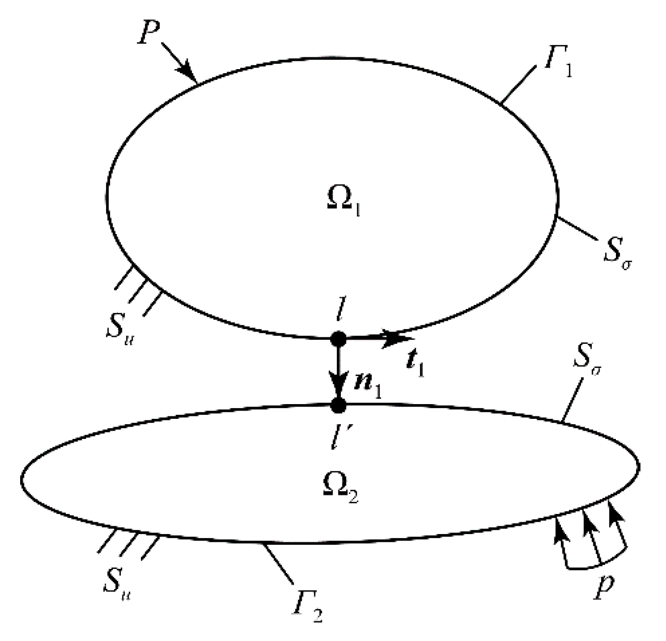
3.1. Contact Conditions

Figure 1 shows a typical contact problem. ${\mathsf{\Omega }}_1$ and ${\mathsf{\Omega }}_2$ are two objects, whose boundaries are ${\Gamma }_1$ and ${\Gamma }_2$, respectively. $S_u$ and $S_{\sigma }$ are the given displacement and stress boundaries, respectively. P and p are the external loads. $l$ and $l^{\prime }$ are a contact point pair and $n_1$ and $t_1$ are the unit normal and tangential vectors of the contact interface, respectively. When the two objects are in contact, the contact system should satisfy the contact displacement and contact force conditions in addition to the boundary and initial conditions. This paper assumes that there is no initial gap between the two objects.

(1)

Contact Displacement Conditions

For two squeezed objects, it is generally considered that they will not embed into each other, so the contact point pair $l$ and $l^{\prime }$ should satisfy the displacement condition of no embedding in the normal direction:

$$n_1^{\mathrm{T}}(U_{l^{\prime }}^{t+\Delta t}-U_l^{t+\Delta t})=0$$

(5)

where $U_{l^{\prime }}^{t+\Delta t}$ and $U_l^{t+\Delta t}$ are the displacement vectors of $l^{\prime }$ and $l$, respectively, at time t + Δt. The direction of $n_1$ is from $l$ to $l^{\prime }$.

For a contact point pair without relative sliding, the displacement condition of no relative sliding in the tangential direction within time t–t + Δt should be satisfied:

$$t_1^{\mathrm{T}}(U_{l^{\prime }}^{t+\Delta t}-U_l^{t+\Delta t})=t_1^{\mathrm{T}}(U_{l^{\prime }}^t-U_l^t)$$

(6)

(2)

Contact Force Conditions

For two objects in contact, the interaction forces between the contact point pair should satisfy Newton′s third law; that is, the following contact force conditions should be satisfied:

$$N_{l^{\prime }}^t=-N_l^t, T_{l^{\prime }}^t=-T_l^t$$

(7)

where $N_{l^{\prime }}^t$ and $N_l^t$ are the normal contact forces of $l^{\prime }$ and $l$, respectively. $T_{l^{\prime }}^t$ and $T_l^t$ are the tangential contact forces of $l^{\prime }$ and $l$, respectively.

3.2. Contact States

The above contact conditions only apply when two objects are in contact, and they do not exist at the same time. There are generally three types of contact states: bond contact, separation, and sliding contact. The static contact state is also considered in this paper.

(1)

Bond Contact State

In the bond contact state, the contact interface has good bond properties and has no relative sliding, so Equations (5)–(7) constitute the contact conditions. In addition, the normal and tangential contact forces should not exceed the ultimate tensile load and shear load, respectively:

$$\Vert N_l^t\Vert \le D^t{f}_{\mathrm{c}}{A}_1$$

(8)

$$\Vert T_l^t\Vert \le D^t({\mu }_{\mathrm{s}}\Vert N_l^t\Vert +f_{\mathrm{c}}{A}_1)$$

(9)

where $f_{\mathrm{c}}$ is the cohesive force of the contact interface, $A_1$ is the control area of $l$, and ${\mu }_{\mathrm{s}}$ is the static friction coefficient of the contact interface.

(2)

Separation State

In the separation state, the bond properties of the contact interface are destroyed, and there is no contact between the two objects. Therefore, the contact interface is not restricted by the contact conditions, giving

$$\Vert N_l^t\Vert =\Vert T_l^t\Vert =0$$

(10)

(3)

Sliding Contact State

In the sliding contact state, the bond properties of the contact interface are destroyed, and there is relative sliding. This state is a sliding friction state, so Equations (5) and (7) constitute the contact conditions. At this point, the tangential contact force should be calculated according to the dynamic friction law:

$$\Vert T_l^t\Vert =D^t{\mu }_{\mathrm{d}}\Vert N_l^t\Vert$$

(11)

where ${\mu }_{\mathrm{d}}$ is the dynamic friction coefficient of the contact interface.

(4)

Static Contact State

In the static contact state, the bond properties of the contact interface are destroyed, but there is no relative sliding. This state is a static friction state, so Equations (5)–(7) constitute the contact conditions. At this point, the tangential contact force should not exceed the ultimate shear load:

$$\Vert T_l^t\Vert \le D^t{\mu }_{\mathrm{s}}\Vert N_l^t\Vert$$

(12)

The above contact conditions are the relationships between the contact displacement and contact force that the contact interface should satisfy when the contact state is known. In the numerical calculation process, the contact state is often not known in advance, so it is necessary to assume and judge it in each calculation step.

4. Dynamic Contact Analysis Method for Rock Mass and Fault

In the seismic loading process of a system, the contact states between the rock mass and the fault can directly affect the seismic safety of the tunnel structure. Based on the point-to-point contact type in the traditional dynamic contact force method, the point-to-surface contact type is also considered in this paper, thus improving the method for studying the nonlinear dynamic large sliding problem between a rock mass and a fault.

4.1. Fundamental Theory of the Dynamic Contact Force Method

According to the basic theory of kinematics, the dynamic balance equation for the contact nodes can be obtained after the tunnel system is discretized using finite elements:

$$M\ddot{U}+F_{\mathrm{damp}}+F_{\mathrm{int}}=F+R$$

(13)

where M is the mass matrix, U is the displacement vector, $F_{\mathrm{damp}}$ is the damping force vector, $F_{\mathrm{int}}$ is the internal force vector, which is obtained by the stress integration of the elements, F is the load vector of the seismic wave, and R is the contact force vector, R = N + T.

When the movement states of the contact nodes are known at time t, the integration schemes of the movement variables at time t + Δt can be obtained, using the explicit central difference method to solve Equation (13):

$$U^{t+\Delta t}={\overline{U}}^{t+\Delta t}+\mathsf{\Delta }{U}^{t+\mathsf{\Delta }t}$$

(14)

$${\dot{U}}^{t+\Delta t}=\frac{2(U^{t+\Delta t}-U^t)}{\Delta t}-{\dot{U}}^t$$

(15)

$${\overline{U}}^{t+\Delta t}=U^t+\Delta t{\dot{U}}^t+\frac{\Delta t^2}{2}{M}^{-1}(F^t-F_{\mathrm{int}}^t-F_{\mathrm{damp}}^t)$$

(16)

$$\mathsf{\Delta }{U}^{t+\Delta t}=\frac{\mathsf{\Delta }{t}^2}{2}{M}^{-1}{R}^t$$

(17)

where ${\overline{U}}^{t+\Delta t}$ is the predicted displacement when ignoring the contact force $R^t$ and $\mathsf{\Delta }{U}^{t+\Delta t}$ is the modified displacement caused by $R^t$.

From the above integration schemes, we can see that the key to determining the movement states of the contact nodes at time t + Δt is solving for their contact force $R^t$. $R^t$ should be determined based on the contact states and the contact conditions between the rock mass and the fault within time t–t + Δt.

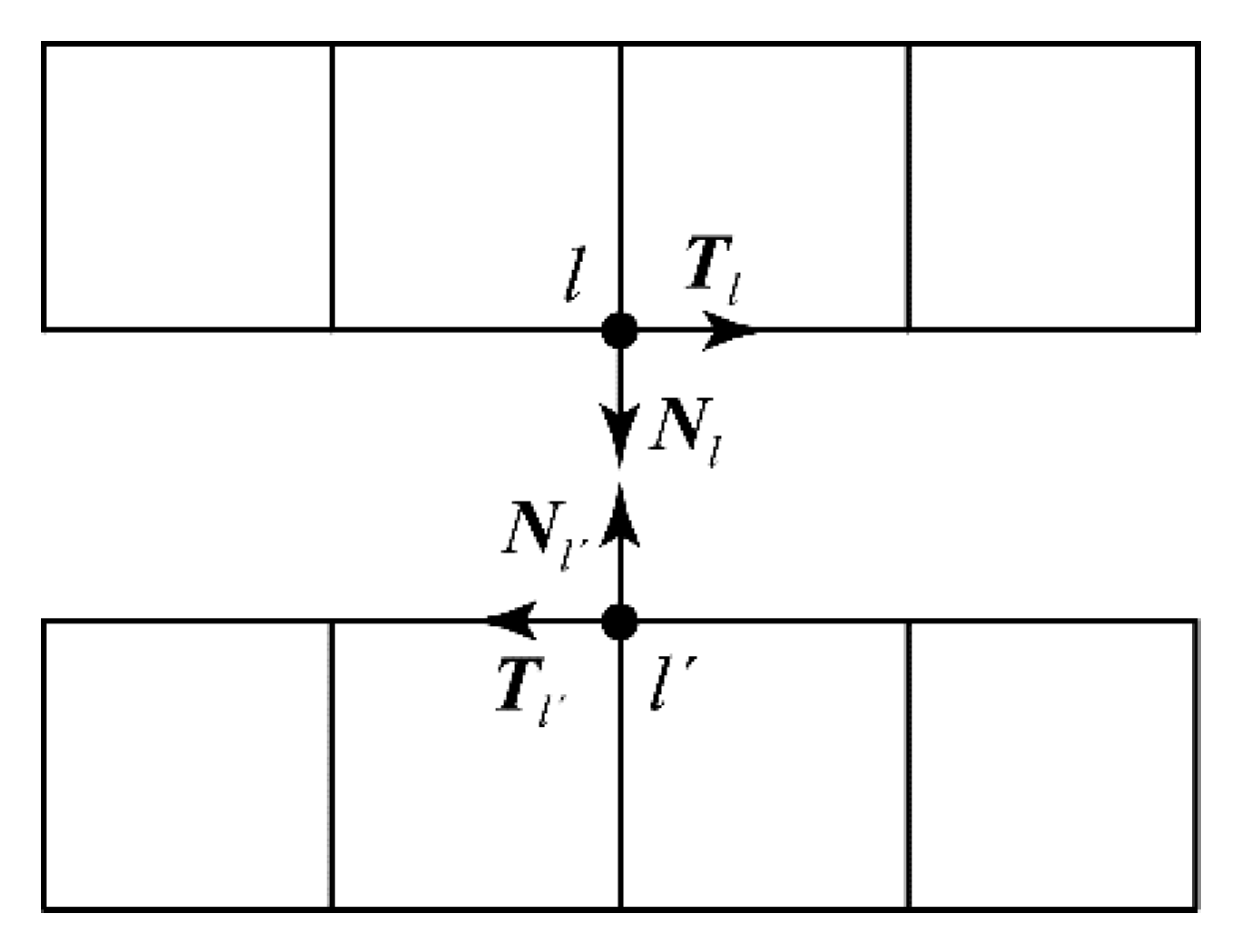
4.2. Solving for the Contact Force and Judging of the Contact State

The point-to-point contact is the most widely used contact type [14] and is very effective in simulating the small sliding problem, but it is difficult to simulate the large sliding problem well using this method. Based on the point-to-point contact type, the calculation formula for the contact force was derived, and methods of judging the contact state were designed. In order to simulate the large sliding problem between the rock mass and the fault, we needed to extend the point-to-point contact method to include the point-to-surface contact.

(1)

Point-to-Point Contact Type

When the contact point pair has no large relative sliding, it can be considered that the contact points are of the point-to-point type (as shown in Figure 2). In order to solve the contact force $R^t$ for this contact type, it can be assumed that the contact points are in the bond contact state. Then, they should satisfy the contact displacement conditions (Equations (5) and (6)). The normal and tangential contact gaps of the contact point pair are denoted ${\mathsf{\Delta }}_{\mathrm{n}}$ and ${\mathsf{\Delta }}_{\mathrm{t}}$, and hence

$${\mathsf{\Delta }}_{\mathrm{n}}=n_1^{\mathrm{T}}({\overline{U}}_{l^{\prime }}^{t+\Delta t}-{\overline{U}}_l^{t+\Delta t}),{ \mathsf{\Delta }}_{\mathrm{t}}=t_1^{\mathrm{T}}[({\overline{U}}_{l^{\prime }}^{t+\Delta t}-{\overline{U}}_l^{t+\Delta t})-(U_{l^{\prime }}^t-U_l^t)]$$

(18)

Combining Equations (5), (6), (14), (17), and (18), and according to the contact force conditions (Equation (7)), the expression for the contact force $R_l^t$ can be derived in the form of a normal component $N_l^t$ and a tangential component $T_l^t$:

$$N_l^t=\frac{2M_l{M}_{l^{\prime }}}{(M_l+M_{l^{\prime }})\mathsf{\Delta }{t}^2}{\mathsf{\Delta }}_{\mathrm{n}}{n}_1, T_l^t=\frac{2M_l{M}_{l^{\prime }}}{(M_l+M_{l^{\prime }})\mathsf{\Delta }{t}^2}{\mathsf{\Delta }}_{\mathrm{t}}{t}_1$$

(19)

where $M_{l^{\prime }}$ and $M_l$ are the lumped masses of $l^{\prime }$ and $l$, respectively.

If ${\mathsf{\Delta }}_{\mathrm{n}}>0$, this indicates that the contact points are in a tension state. If $N_l^t$ satisfies Equation (8), this assumption is correct; otherwise, the contact points enter a separation state, and then the contact force is modified according to Equation (10). If ${\mathsf{\Delta }}_{\mathrm{n}}\le 0$, this indicates that the contact points are in a compression state. If $T_l^t$ satisfies Equation (9), this assumption is correct; otherwise, the contact points enter a sliding contact state, and then the contact force is modified according to Equation (11).

(2)

Point-to-Surface Contact Type

When the contact point pair has large relative sliding, it can be considered that the contact points are of the point-to-surface type (as shown in Figure 3), and the cohesive force is no longer considered in this case. In order to solve for the contact force $R^t$, it can be assumed that the contact points are in a static contact state, so they should satisfy the contact displacement conditions (Equations (5) and (6)). Assuming that $l^{\prime }$ is the projection point of $l$ on the contact interface, the displacement of $l^{\prime }$ is given by

$$U_{l^{\prime }}^t={\displaystyle \sum _p{\Phi }_p{U}_p^t}$$

(20)

where p is the node number of the element to which the contact interface belongs, ${\Phi }_p$ is the shape-function value of p and $M_{l^{\prime }}$ is the equivalent lumped mass of $l^{\prime }$, as shown below [24].

$$M_{l^{\prime }}={\displaystyle \sum _p{m}_p}, m_p=\frac{M_p{\Phi }_p}{{\displaystyle \sum _q{\Phi }_q^2}}$$

(21)

where $m_p$ is the mass contribution of p, $M_p$ is the lumped mass of p, and q has the same meaning as p.

According to the contact conditions, the expression for the contact force $R_l^t$ can also be derived in the form of Equation (19). The contact force of p is calculated via

$$N_p^t=\frac{m_p}{M_{l^{\prime }}}{N}_{l^{\prime }}^t, T_p^t=\frac{m_p}{M_{l^{\prime }}}{T}_{l^{\prime }}^t$$

(22)

If ${\mathsf{\Delta }}_{\mathrm{n}}>0$, this indicates that the contact points enter a separation state, and then the contact force is modified according to Equation (10). If ${\mathsf{\Delta }}_{\mathrm{n}}\le 0$, this indicates that the contact points are in a compression state. If $T_l^t$ satisfies Equation (12), this assumption is correct; otherwise, the contact points enter a sliding contact state, and then the contact force is modified according to Equation (11).

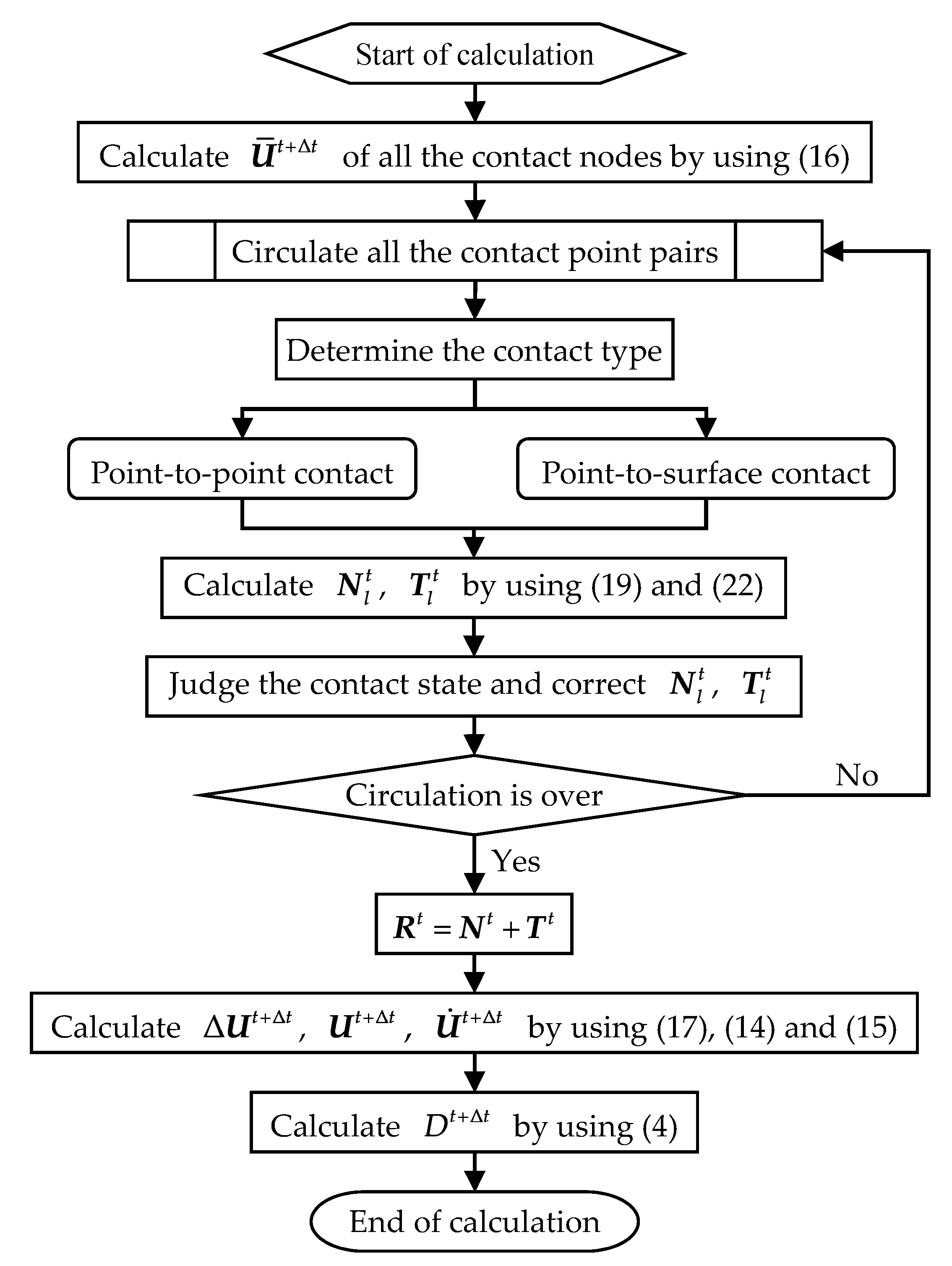
4.3. Calculation Flow of the Improved Dynamic Contact Force Method

Before the seismic action is applied, the discontinuity of the finite element model can be realized by adding common nodes on the contact interface between the rock mass and the fault. The main calculation procedures for the improved dynamic contact force method are: (1) calculate the predicted displacement ${\overline{U}}^{t+\Delta t}$, ignoring the contact force $R^t$; (2) determine the contact types of all the contact point pairs; (3) use the improved method to calculate and modify $R^t$; (4) calculate the modified displacement $\mathsf{\Delta }{U}^{t+\Delta t}$ caused by $R^t$; (5) calculate the vibration deterioration coefficient $D^{t+\mathsf{\Delta }t}$. The dynamic finite element calculation flow for the tunnel contact system at time t + Δt is shown in Figure 4.

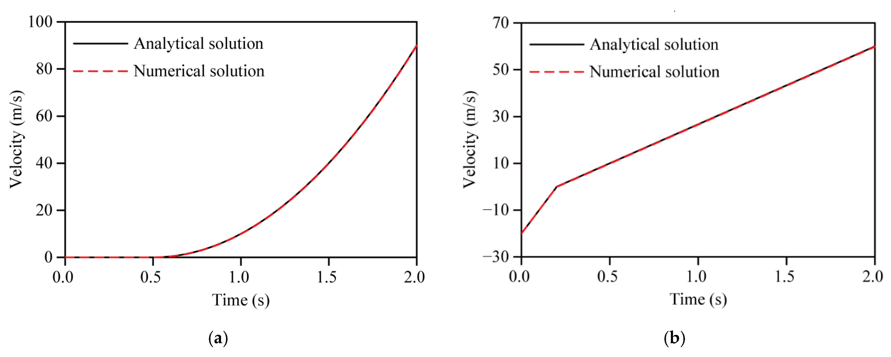
5. Verification of the Method

In order to verify the accuracy of the improved dynamic contact force method for simulating large sliding displacements, the movement response of a sliding block under external loads (as shown in Figure 5) was selected for analysis [25]. The block was a cube with an edge length of 1.0 m, and the sliding surface under the block was sufficiently large. The block and the bottom surface were made of the same linear elastic material, with an elastic modulus of 0.3 GPa, a Poisson ratio of 0.3, and a density of 300 kg/m³. The finite element mesh was composed of hexahedral elements with dimensions of 0.5 m × 0.5 m × 0.5 m. It was assumed that the gravity of the block, the cohesive force of the sliding surface, and the vibration deterioration effect of the sliding surface need not be considered. The static and dynamic friction coefficients of the sliding surface were approximately equal. In order to investigate the mutual transformation of different contact states, two calculation cases were designed, as shown in

Table 1. Design of calculation cases.

Case	Initial Displacement ${\mathit{U}}^0 \left(\mathrm{m}\right)$	Initial Velocity ${\dot{\mathit{U}}}^0 (\mathrm{m}·{\mathrm{s}}^{-1})$	Vertical Load ${\mathit{F}}_{\mathrm{N}} \left(\mathrm{kN}\right)$	Horizontal Load ${\mathit{F}}_{\mathrm{T}} \left(\mathrm{kN}\right)$	Friction Coefficient $\mu$
1	0	0	−30	24 t	0.4
2	0	−20	−25	20	0.4

(where t is the time).

Taking the bottom center of the block as a monitoring point (as shown by the red dot in Figure 5), the velocity and displacement time histories of the block, calculated by the method developed in this paper and the analytical method, are plotted in Figure 6 and Figure 7. In the two calculation cases, the numerical solutions of the velocity and displacement time histories of the block were basically consistent with the analytical solutions. The results show that under the above assumption, the improved dynamic contact force method is feasible, and is suitable for simulating different contact states of a contact system and the large sliding problem for contact interfaces.

6. Engineering Case Study

6.1. Engineering Profiles and Calculation Model

The water diversion project of Central Yunnan is a super-large inter-basin water transfer project, which takes water from the Shigu segment of the upper reaches of the Jinsha River to solve the water shortage problem in the Central Yunnan areas. The control project for the main canal is the Xianglushan tunnel in Dali section I, with a total length of 63.43 km and a buried depth of more than 300 m. Many active fault zones exist along the line, most of which intersect with the line at medium or large angles. The basic earthquake intensity degree of the tunnel area is degree 8, and the peak acceleration of the horizontal ground motion with 10% exceedance probability in 50 years is 0.2–0.3 g. A tunnel section with a fault and a buried depth of 400 m was selected for the seismic calculation in this study. The rock mass is type IV, and the tunnel diameter is 9.8 m. The thickness of the lining support is 55 cm, with a C30 concrete structure.

Due to the great depth of the tunnel, the number of elements would be very large and the dynamic calculation would take a great deal of time if the 3D finite element model was built to the ground surface. Therefore, a depth of only 55 m was used at the top of the tunnel, to save calculation time. A normal fault with a thickness of 20 m and a dip angle of 60° was considered, with an inclination parallel to the tunnel axis. The finite element model was composed of 69,888 rock mass elements, 17,472 fault elements, and 8640 lining elements, all of which were eight-node hexahedrons, as shown in Figure 8. The maximum mesh size was within 5 m, which satisfies the accuracy requirement of the dynamic calculation. The initial contact node pairs were set between the hanging wall, the fault, and the footwall, respectively. It should be noted that the contact interface between the concrete lining and the fault or the rock mass was not considered.

Based on a comprehensive analysis of in situ stress test results in the tunnel area, the lateral pressure coefficients of the rock mass were taken as: $k_X$ = 1.2, $k_Y$ = 0.74, $k_Z$ = 1.0. The values of the mechanical parameters of the tunnel materials are provided in

Table 2. Mechanical parameters of tunnel materials.

Material	Elastic Modulus (GPa)	Poisson Ratio	Internal Friction Angle (°)	Cohesive Force (MPa)	Tensile Strength (MPa)	Compressive Strength (MPa)	Density (g∙cm−3)
Fault	0.3	0.33	24.2	0.1	0.50	10.0	2.0
Lining	30.0	0.17	46.0	2.0	1.43	12.7	2.5
Rock	5.0	0.29	35.0	0.6	1.30	40.0	2.7

. The cohesive force of the contact interface between the rock mass and the fault was taken as 0.35 MPa, and the static and dynamic friction coefficients were both taken as 0.53. The undetermined coefficients in Equation (4) were taken as: α = 0.883, β = 0.02, λ = 0.032, $P_0$ = 0.8, ξ = 5. As the research was limited by current test conditions, the values of these undetermined coefficients were mainly based on the test fitting curves in [19,23].

6.2. Calculation Conditions

Based on the improved dynamic contact force method, a seismic response process simulation of the Xianglushan tunnel with a normal fault was performed, using the dynamic time history finite element analysis program for an underground cavern [26]. The same elastoplastic damage constitutive relation was applied to the rock mass and the concrete lining, and the Mohr–Coulomb yield function with a tensile cut-off limit was applied as the yield condition, expressed as

$$f^{\mathrm{s}}={\sigma }_1-{\sigma }_3{N}_{\phi }+2(1-D)c\sqrt{N_{\phi }},f^{\mathrm{t}}={\sigma }_3-{\sigma }^{\mathrm{t}}$$

(23)

where $f^{\mathrm{s}}=0$ and $f^{\mathrm{t}}=0$ represent the shear and tensile yield conditions, respectively, and ${\sigma }_3$ and ${\sigma }_1$ are the maximum and minimum principal stresses, respectively. It was assumed that tensile stress is positive and compressive stress is negative. In addition, c is the cohesive force, ${\sigma }^{\mathrm{t}}$ is the tensile strength and $N_{\phi }$ is a parameter expressed as

$$N_{\phi }=\frac{1+\sin \phi }{1-\sin \phi }$$

(24)

where φ is the internal friction angle. D is the damage coefficient, which is expressed as

$$D=\sqrt{D_1^2+D_2^2+D_3^2}$$

(25)

$$D_i=1-\exp (-R\sqrt{{\epsilon }_i^p{\epsilon }_i^p}), i=1,2, 3$$

(26)

where $D_i$ is the damage coefficient of the i-th principal stress direction, ${\epsilon }_i^p$ is the cumulative plastic deviator strain of the i-th principal strain direction and R is a dimensionless constant.

A free field artificial boundary condition was applied at the four vertical boundaries, and a viscoelastic artificial boundary condition was applied at the top and bottom of the finite element model.

In this study, a representative Kobe NS wave was selected for input to the model in the form of acceleration time histories. A duration section of 15 s with high amplitude was adopted to shorten the calculation time. Then, the amplitude of the input wave was adjusted to 0.15 g to meet the requirements of seismic fortification intensity and the amplitude reduction of a deep tunnel. The processed acceleration time histories are shown in Figure 9, where only the x-direction seismic excitation is considered.

In addition, a contrasting calculation case was designed, with no contact node pairs between the rock mass and the fault. In other words, the rock mass and the fault were regarded as a continuous structure. Then, the seismic responses of the tunnel in the two calculation cases (considering or ignoring the dynamic interaction between the rock mass and the fault (with RFI or without RFI)) were analyzed comparatively. In order to monitor the displacement and stress time histories of the lining, three monitoring points were set at typical parts of the lining: the bottom arch, the haunch, and the top arch at the middle position of the fault. It should be noted that the tunnel excavation and the lining support calculations should be performed before the seismic action is applied.

6.3. Analysis of Calculation Results

6.3.1. Relative Movement and Seismic Deterioration Analysis of the Contact Interface

In the seismic loading process of the system, the relative displacement and relative velocity between the rock mass and the fault leads to the seismic deterioration of the contact interface. A contact node pair close to the lining haunch was selected at the contact interface between the hanging wall and the fault, to monitor the relative movement characteristics of the rock mass and the fault. With the dynamic interaction included, the time histories for the relative x-direction movement of the contact interface between the hanging wall and the fault are plotted in Figure 10, and the time history of the vibration deterioration coefficient of the contact interface is plotted in Figure 11.

We can see from Figure 10a that the relative displacement of the contact interface was very small at time 0–1.5 s, and it fluctuated violently and increased sharply at time 1.5–6.0 s. The maximum relative displacement was −5.14 cm, appearing at time 4.9 s. After time 6.0 s, the relative displacement basically remained at −4.40 cm. This indicates that the movements of the rock mass and the fault were not synchronous under a large seismic action, and an obvious dislocation displacement appeared between them. That is to say, the rock mass and the fault were in a sliding contact state after time 6.0 s. We can see from Figure 10b that the relative velocity of the contact interface presented similar fluctuating change laws, due to the fluctuation of the input wave: the relative velocity fluctuated violently at time 1.5–6.0 s and fluctuated gently after time 6.0 s.

We can see from Figure 11 that the vibration deterioration coefficient of the contact interface presented clear negative exponential attenuation laws over time: the coefficient decreased rapidly at time 0–1.5 s, then decreased to a certain extent at time 1.5–6.0 s, tending to be stable after time 6.0 s. This indicates that the seismic deterioration effect of the contact interface accumulated gradually over time, and its deterioration degree can be directly reflected in the value of the vibration deterioration coefficient.

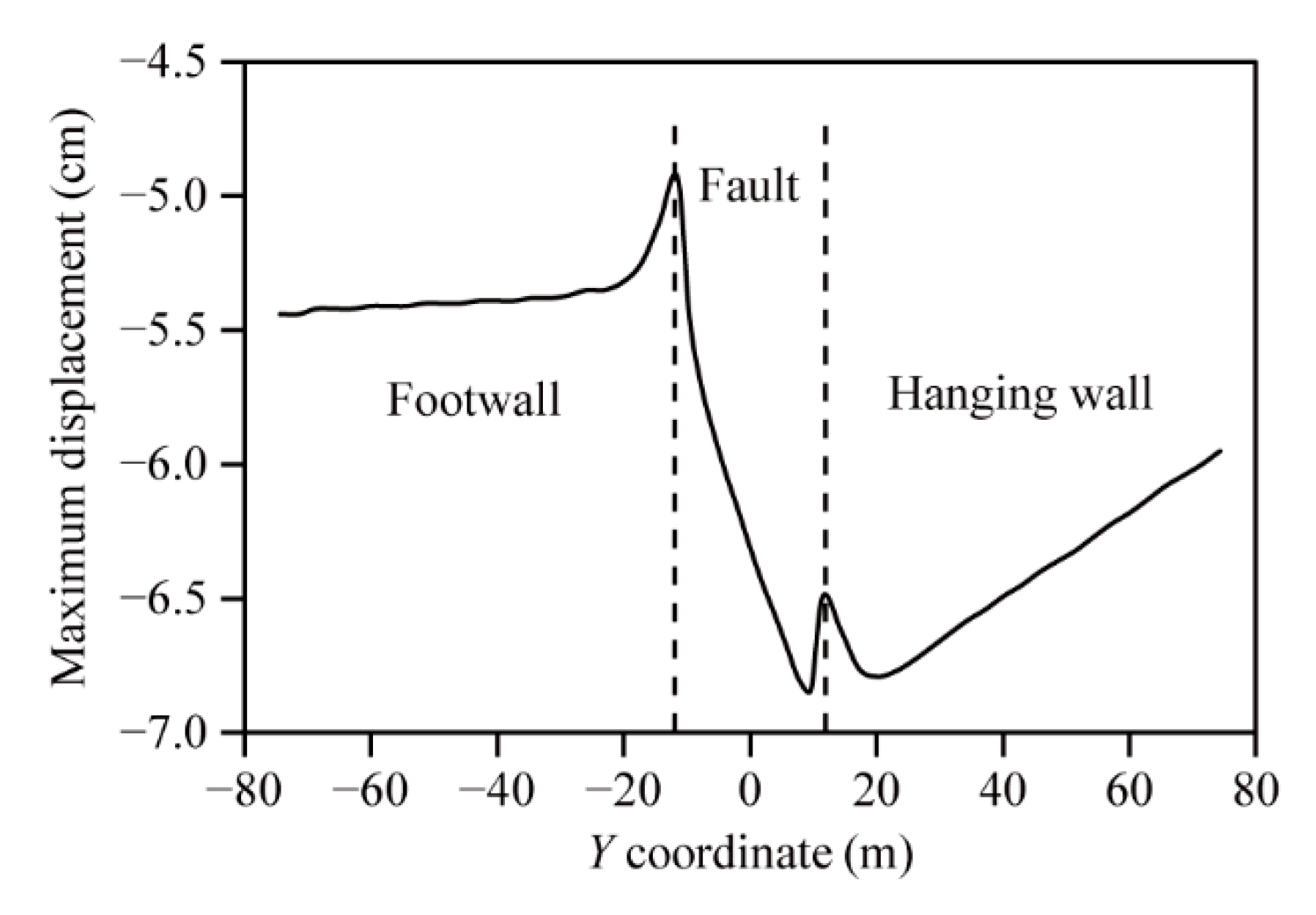
6.3.2. Displacement Analysis of the Lining

With the dynamic interaction between the rock mass and the fault considered or ignored, the time histories of the x-direction displacement of the lining monitoring points in the two calculation cases are plotted in Figure 12.

We can see from Figure 12 that the movement laws of the three typical parts were basically the same, and only the magnitudes at each point in time were somewhat different. On the whole, the displacement time histories of the bottom arch and the top arch were basically the same, while the displacement of the haunch along the x-direction was larger than that of the other parts. The main reason for this is that, influenced by the spatial structure of the tunnel, the seismic response of the haunch was more intense than that of the other parts under a transverse seismic wave. When the dynamic interaction between the rock mass and the fault was ignored, the maximum displacement of the haunch was −6.16 cm, appearing at time 3.0 s, and the maximum relative displacement between the haunch and the bottom arch was −0.33 cm. When the dynamic interaction was considered, the maximum displacement of the haunch was −6.31 cm, also appearing at time 3.0 s, and the maximum relative displacement between the haunch and the bottom arch was −0.64 cm. In the two calculation cases, the displacement responses of the lining are clearly different. The main reason for this is that an obvious transverse dislocation displacement appears between the rock mass and the fault under seismic action, which has an important influence on the seismic response of the lining monitoring section, especially the displacement of the haunch. This indicates that the transverse dislocation displacement between the rock mass and the fault leads to large relative deformations between different parts of the lining. Therefore, considering the dynamic interaction between the rock mass and the fault can more objectively reflect the displacement response characteristics of the tunnel structure.

According to the above analysis, the displacement of the lining haunch along the x-direction reached a maximum at time 3.0 s. With the dynamic interaction between the rock mass and the fault considered, the changing laws of the transverse maximum displacement of the haunch along the tunnel axis at time 3.0 s are plotted in Figure 13. Here, the minus sign indicates the direction.

We can see from Figure 13 that the maximum displacements of the haunch at different y coordinates of the footwall were basically the same. From the footwall to the fault, the displacement decreased sharply at the contact interface, and increased rapidly at the fault. From the fault to the hanging wall, the displacement appeared to change suddenly at the contact interface, decreasing slowly at the hanging wall. This indicates that the displacement of the lining was greatly affected by the fault dislocation, especially near the contact interface. Compared with the lining at the footwall, the fault was more likely to affect the lining at the hanging wall, which was characterized by a larger displacement.

6.3.3. Stress and Damage Analysis of the Lining

In view of the fact that the tensile strength of concrete is much smaller than its compressive strength, only the changing laws of the tensile stress of the lining were analyzed in this study, which is reflected in the maximum principal stress. With the dynamic interaction between the rock mass and the fault considered or ignored, the time histories of the maximum principal stress of the lining monitoring points in the two calculation cases are plotted in Figure 14.

We can see from Figure 14 that the changing laws of the maximum principal stress of the three typical parts were basically the same: the stress increased slowly at time 0–1.5 s, then changed and increased rapidly at time 1.5–6.0 s, changing little after time 6.0 s. On the whole, the tensile stress of the haunch was larger than that of the other parts. The maximum tensile stress of the lining was 1.05 MPa when the dynamic interaction between the rock mass and the fault was ignored, while the value was 1.43 MPa when the dynamic interaction was considered, which is clearly larger than that in the former case. In addition, when the dynamic interaction was considered, the maximum tensile stress of the haunch reached the tensile strength of concrete, and the haunch may then suffer damage. This indicates that the stress of the lining is greatly affected by the dislocation displacement between the rock mass and the fault.

According to the above analysis, tensile damage appears on the lining when the dynamic interaction between the rock mass and the fault is considered. Based on the damage constitutive relation of concrete, the distribution of the damage coefficient of the lining structure after the earthquake can be obtained, as shown in Figure 15, and the changing laws of the damage coefficient of the lining haunch along the tunnel axis after the earthquake are plotted in Figure 16.

We can see from Figure 15 and Figure 16 that the damage area of the lining was mainly distributed in a certain range near both sides of the fault and at the parts where the fault passes through, especially at the haunch. From the footwall to the fault, the damage coefficient of the haunch first increased and then decreased. From the fault to the hanging wall, the damage coefficient of the haunch also first increased and then decreased. Compared with the other parts, the damage to the lining at the contact interface between the rock mass and the fault was the most serious. Compared with the contact interface between the footwall and the fault, the damage to the lining at the contact interface between the hanging wall and the fault was more serious. The local damage coefficient of the haunch at this part was close to 1.0, and the haunch may then crack. Based on the above analysis, the influences of fault dislocations should be considered in the seismic design of a tunnel structure through a fault, from the perspective of engineering safety. In addition, according to the distribution length of the damage area of the lining, the longitudinal layout range of seismic fortification for the tunnel structure can be determined.

6.4. Discussion

The seismic response of the tunnel through fault is affected by many factors, including fault thickness and fault dip angle. In this section, when the influences of different fault thicknesses on the seismic response of the tunnel were considered, the fault dip angle was uniformly set at 60°. When the influences of different fault dip angles on the seismic response of the tunnel were considered, the fault thickness was uniformly set at 20 m. In all the above calculation cases, the other calculation conditions remained consistent, including the fact that the dynamic interaction between the rock mass and the fault was considered.

6.4.1. Influences of Fault Thickness on Seismic Response of the Lining

The maximum displacements and maximum tensile stresses of the lining monitoring points under different fault thicknesses are plotted in Figure 17, and the damage coefficients of the haunch monitoring point under different fault thicknesses are plotted in Figure 18.

We can see from Figure 17 that as the fault thickness increased, the maximum displacements of the three typical parts decreased gradually, tending to be stable when the thickness exceeded 30 m. Similarly, the changing of the maximum tensile stresses with fault thickness showed the same laws. This is mainly because the larger the fault thickness, the farther the lining monitoring section from the contact interface between the rock mass and the fault, so that the influence of the fault dislocation on the monitoring points is smaller. When the fault thickness exceeds a certain size, the influence of the fault dislocation on the monitoring points can be ignored. It should be noted that the maximum tensile stress of the haunch reached the tensile strength of concrete when the fault thickness did not exceed 20 m, and this part may then suffer damage. Furthermore, we can see from Figure 18 that as the fault thickness increased, the damage coefficient of the lining haunch decreased gradually, remaining at zero when the thickness exceeded 30 m.

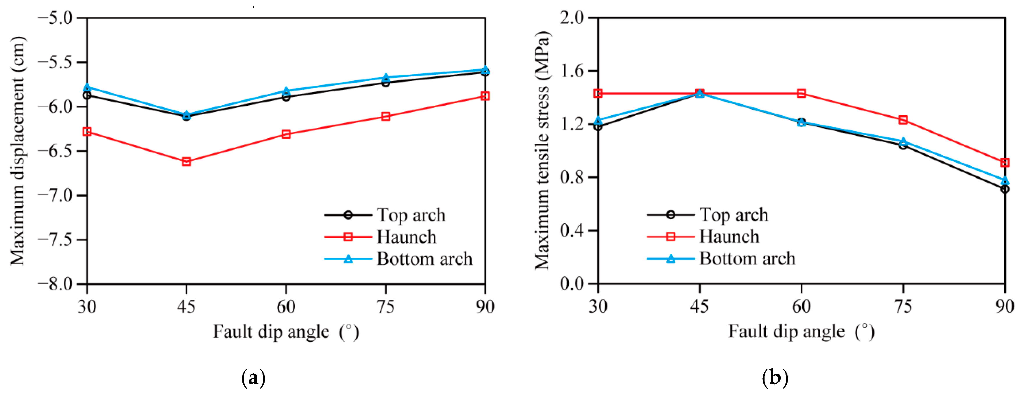
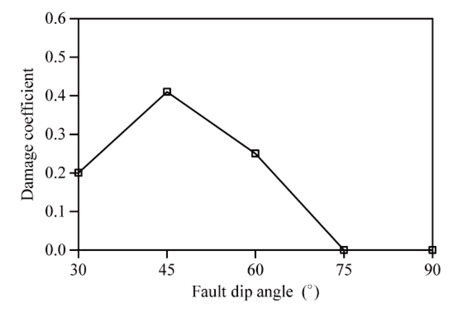
6.4.2. Influences of Fault Dip Angle on Seismic Response of the Lining

The maximum displacements and maximum tensile stresses of the lining monitoring points under different fault dip angles are plotted in Figure 19, and the damage coefficients of the haunch monitoring point under different fault dip angles are plotted in Figure 20.

We can see from Figure 19 that as the fault dip angle increased, both the maximum displacements and maximum tensile stresses of the three typical parts first increased and then decreased, reaching a maximum at 45°. This indicates that the fault dip angle had a great influence on the seismic response of the lining monitoring section. It should be noted that the maximum tensile stress of the haunch reached the tensile strength of concrete when the fault dip angle did not exceed 60°, and this part may then suffer damage. Furthermore, we can see from Figure 20 that as the fault dip angle increased, the damage coefficient of the lining haunch first increased and then decreased, reaching a maximum at 45°. When the fault dip angle exceeded 75°, the damage coefficient of the lining haunch remained zero.

7. Conclusions

(1) Considering the dynamic deterioration characteristics of a rock structural plane under seismic action, a mathematical model reflecting the seismic deterioration effect of the contact interface between the rock mass and the fault was established. Based on the point-to-point contact type in the traditional dynamic contact force method, the point-to-surface contact type was also considered, and an improved dynamic contact force method considering the large sliding characteristics of the contact interface was established. Then, a nonlinear dynamic simulation method for the rock–fault contact system was developed. The calculation flow of the improved dynamic contact force method was designed, and the accuracy of the method was verified using the example of a sliding elastic block.

(2) Based on the improved dynamic contact force method, the nonlinear seismic damage characteristics of a deep tunnel through a normal fault were studied. The relative movement and seismic deterioration effect of the contact interface between the rock mass and the fault, and the characteristics of displacement, stress, and damage to the lining, were analyzed. The results indicated that the movements of the rock mass and the fault were not synchronous under large seismic action, and the seismic deterioration effect of the contact interface accumulated gradually over time. The proposed method can effectively simulate the vibration deterioration degree of the contact interface and the nonlinear large sliding problem of the rock–fault contact system.

(3) When the dynamic interaction between the rock mass and the fault was considered, the displacement and stress responses of the lining were greatly affected by the transverse dislocation displacement between the two, shown by a clear increase in the values. Compared with the lining at the footwall, the displacement of the lining at the hanging wall was more easily affected by the fault. Tensile damage appeared on the lining in the seismic loading process, and the damage area of the lining was mainly distributed in a certain range near both sides of the fault and at the parts where the fault passes through, especially at the haunch. Compared with the contact interface between the footwall and the fault, the damage to the lining at the contact interface between the hanging wall and the fault was more serious. This indicates that considering the dynamic interaction between rock mass and fault can more objectively reflect the seismic response characteristics of the tunnel structure.

(4) The influences of different fault thicknesses and different fault dip angles on the seismic response of the tunnel structure were discussed. As the fault thickness increased, both the maximum displacements and the maximum tensile stresses of the lining monitoring points decreased gradually, tending to be stable when the thickness exceeded 30 m. The damage coefficient of the lining haunch decreased gradually, and remained zero when the fault thickness exceeded 30 m. As the fault dip angle increased, both the maximum displacements and maximum tensile stresses of the lining monitoring points first increased and then decreased, reaching a maximum at 45°. The damage coefficient of the lining haunch first increased and then decreased, reaching a maximum when the fault dip angle was 45° and remaining zero when the fault dip angle exceeded 75°.

References

1. Huang, J.Q.; Zhao, M.; Du, X.L. Non-linear seismic responses of tunnels within normal fault ground under obliquely incident P waves. Tunn. Undergr. Space Technol. 2017, 61, 26–39. [Google Scholar] [CrossRef]
2. Wang, Z.Z.; Zhang, Z. Seismic damage classification and risk assessment of mountain tunnels with a validation for the 2008 Wenchuan earthquake. Soil Dyn. Earthq. Eng. 2013, 45, 45–55. [Google Scholar] [CrossRef]
3. Yan, G.M.; Gao, B.; Shen, Y.S.; Zheng, Q.; Fan, K.X.; Huang, H.F. Shaking table test on seismic performances of newly designed joints for mountain tunnels crossing faults. Adv. Struct. Eng. 2020, 23, 248–262. [Google Scholar] [CrossRef]
4. Shen, Y.S.; Gao, B.; Yang, X.M.; Tao, S.J. Seismic damage mechanism and dynamic deformation characteristic analysis of mountain tunnel after Wenchuan earthquake. Eng. Geol. 2014, 180, 85–98. [Google Scholar] [CrossRef]
5. Li, T.B. Damage to mountain tunnels related to the Wenchuan earthquake and some suggestions for aseismic tunnel construction. Bull. Eng. Geol. Environ. 2012, 71, 297–308. [Google Scholar] [CrossRef]
6. Yu, H.T.; Chen, J.T.; Bobet, A.; Yuan, Y. Damage observation and assessment of the Longxi tunnel during the Wenchuan earthquake. Tunn. Undergr. Space Technol. 2016, 54, 102–116. [Google Scholar] [CrossRef]
7. Fang, L.; Jiang, S.P.; Lin, Z.; Wang, F.Q. Shaking table model test study of tunnel through fault. Rock Soil Mech. 2011, 32, 2709–2713. [Google Scholar]
8. Liu, Y.; Gao, F. Experimental study on the dynamic characteristics of a tunnel-crossing fault using a shake-table test. J. Vib. Shock. 2016, 35, 160–165. [Google Scholar]
9. Fan, L.; Chen, J.L.; Peng, S.Q.; Qi, B.X.; Zhou, Q.W.; Wang, F. Seismic response of tunnel under normal fault slips by shaking table test technique. J. Cent. South. Univ. 2020, 27, 1306–1319. [Google Scholar] [CrossRef]
10. Li, L.; He, C.; Geng, P.; Cao, D.J. Analysis of seismic dynamic responses of tunnel through fault zone in high earthquake intensity area. J. Chongqing Univ. Nat. Sci. Ed. 2012, 35, 92–98. [Google Scholar]
11. Yang, Z.H.; Lan, H.X.; Zhang, Y.S.; Gao, X.; Li, L.P. Nonlinear dynamic failure process of tunnel-fault system in response to strong seismic event. J. Asian Earth Sci. 2013, 64, 125–135. [Google Scholar] [CrossRef]
12. Ardeshiri-Lajimi, S.; Yazdani, M.; Langroudi, A.A. Control of fault lay-out on seismic design of large underground caverns. Tunn. Undergr. Space Technol. 2015, 50, 305–316. [Google Scholar] [CrossRef]
13. Liu, J.B.; Sharan, S.K. Analysis of dynamic contact of cracks in viscoelastic media. Comput. Methods Appl. Mech. Eng. 1995, 121, 187–200. [Google Scholar] [CrossRef]
14. Yang, Y.; Chen, J.T.; Xiao, M. Analysis of seismic damage of underground powerhouse structure of hydropower plants based on dynamic contact force method. Shock. Vib. 2014, 2014, 1–13. [Google Scholar] [CrossRef]
15. Zhou, H.; Xiao, M.; Yang, Y.; Liu, G.Q. Seismic response analysis method for lining structure in underground cavern of hydropower station. KSCE J. Civ. Eng. 2019, 23, 1236–1247. [Google Scholar] [CrossRef]
16. Hutson, R.W.; Dowding, C.H. Joint asperity degradation during cyclic shear. Int. J. Rock Mech. Min. Sci. 1990, 27, 109–119. [Google Scholar] [CrossRef]
17. Hou, D.; Rong, G.; Yang, J.; Zhou, C.B.; Peng, J.; Wang, X.J. A new shear strength criterion of rock joints based on cyclic shear experiment. Eur. J. Environ. Civ. Eng. 2016, 20, 180–198. [Google Scholar] [CrossRef]
18. Yang, Z.Y.; Di, C.C.; Yen, K.C. The effect of asperity order on the roughness of rock joints. Int. J. Rock Mech. Min. Sci. 2001, 38, 745–752. [Google Scholar] [CrossRef]
19. Ni, W.D.; Tang, H.M.; Liu, X.; Wu, Y.P. Dynamic stability analysis of rock slope considering vibration deterioration of structural planes under seismic loading. Chin. J. Rock Mech. Eng. 2013, 32, 492–500. [Google Scholar]
20. Crawford, A.M.; Curran, J.H. The influence of shear velocity on the frictional resistance of rock discontinuities. Int. J. Rock Mech. Min. Sci. 1981, 18, 505–515. [Google Scholar] [CrossRef]
21. Wang, Z.; Gu, L.L.; Shen, M.R.; Zhang, F.; Zhang, G.K.; Deng, S.X. Influence of shear rate on the shear strength of discontinuities with different joint roughness coefficients. Geotech. Test. J. 2020, 43, 683–700. [Google Scholar] [CrossRef]
22. Lee, H.S.; Park, Y.J.; Cho, T.F.; You, K.H. Influence of asperity degradation on the mechanical behavior of rough rock joints under cyclic shear loading. Int. J. Rock Mech. Min. Sci. 2001, 38, 967–980. [Google Scholar] [CrossRef]
23. Li, H.B.; Feng, H.P.; Liu, B. Study on strength behaviors of rock joints under different shearing deformation velocities. Chin. J. Rock Mech. Eng. 2006, 25, 2435–2440. [Google Scholar]
24. Wang, F.J.; Cheng, J.G.; Yao, Z.H.; Huang, C.J.; Kou, Z.J. A new contact algorithm for numerical simulation of structure crashworthiness. Eng. Mech. 2002, 19, 130–134. [Google Scholar]
25. Zhang, L.H.; Liu, T.Y.; Li, Q.B.; Chen, T. Modified dynamic contact force method under reciprocating load. Eng. Mech. 2014, 31, 8–14. [Google Scholar]
26. Zhang, Z.G.; Xiao, M.; Chen, J.T. Simulation of earthquake disaster process of large-scale underground caverns using three-dimensional dynamic finite element method. Chin. J. Rock Mech. Eng. 2011, 30, 509–523. [Google Scholar]
Figure 1. Contact sketch of two objects.
Energies 14 06700 g001
Figure 2. Point-to-point contact.
Energies 14 06700 g002
Figure 3. Point-to-surface contact.
Energies 14 06700 g003
Figure 4. Calculation flow for the dynamic contact system of tunnel at time t + Δt.
Energies 14 06700 g004
Figure 5. Contact model of the elastic block.
Energies 14 06700 g005
Figure 6. Velocity time histories of the elastic block: (a) case 1; (b) case 2.
Energies 14 06700 g006
Figure 7. Displacement time histories of the elastic block: (a) case 1; (b) case 2.
Energies 14 06700 g007
Figure 8. Three-dimensional calculation model of the tunnel with a normal fault: (a) whole model; (b) lining.
Energies 14 06700 g008
Figure 9. Time history of x-direction acceleration of the input wave.
Energies 14 06700 g009
Figure 10. Time histories of the relative movement of the contact interface between the hanging wall and the fault: (a) displacement; (b) velocity.
Energies 14 06700 g010
Figure 11. Time history of the vibration deterioration coefficient of the contact interface.
Energies 14 06700 g011
Figure 12. Time histories of the x-direction displacement of the monitoring points: (a) without RFI; (b) with RFI.
Energies 14 06700 g012
Figure 13. Changing laws of the maximum displacement of the haunch along the tunnel axis.
Energies 14 06700 g013
Figure 14. Time histories of the maximum principal stress of the monitoring points: (a) without RFI; (b) with RFI.
Energies 14 06700 g014
Figure 15. Distribution of the damage coefficient of the lining after the earthquake.
Energies 14 06700 g015
Figure 16. Changing laws of the damage coefficient of the lining haunch along the tunnel axis.
Energies 14 06700 g016
Figure 17. Maximum response values of the monitoring points under different fault thicknesses: (a) displacement; (b) tensile stress.
Energies 14 06700 g017
Figure 18. Damage coefficients of the haunch monitoring point under different fault thicknesses.
Energies 14 06700 g018
Figure 19. Maximum response values of the monitoring points under different fault dip angles: (a) displacement; (b) tensile stress.
Energies 14 06700 g019
Figure 20. Damage coefficients of the haunch monitoring point under different fault dip angles.
Energies 14 06700 g020