
Evaluation of Ground Motion Amplification Effects in Slope Topography Induced by the Arbitrary Directions of Seismic Waves


Abstract
:1. Introduction
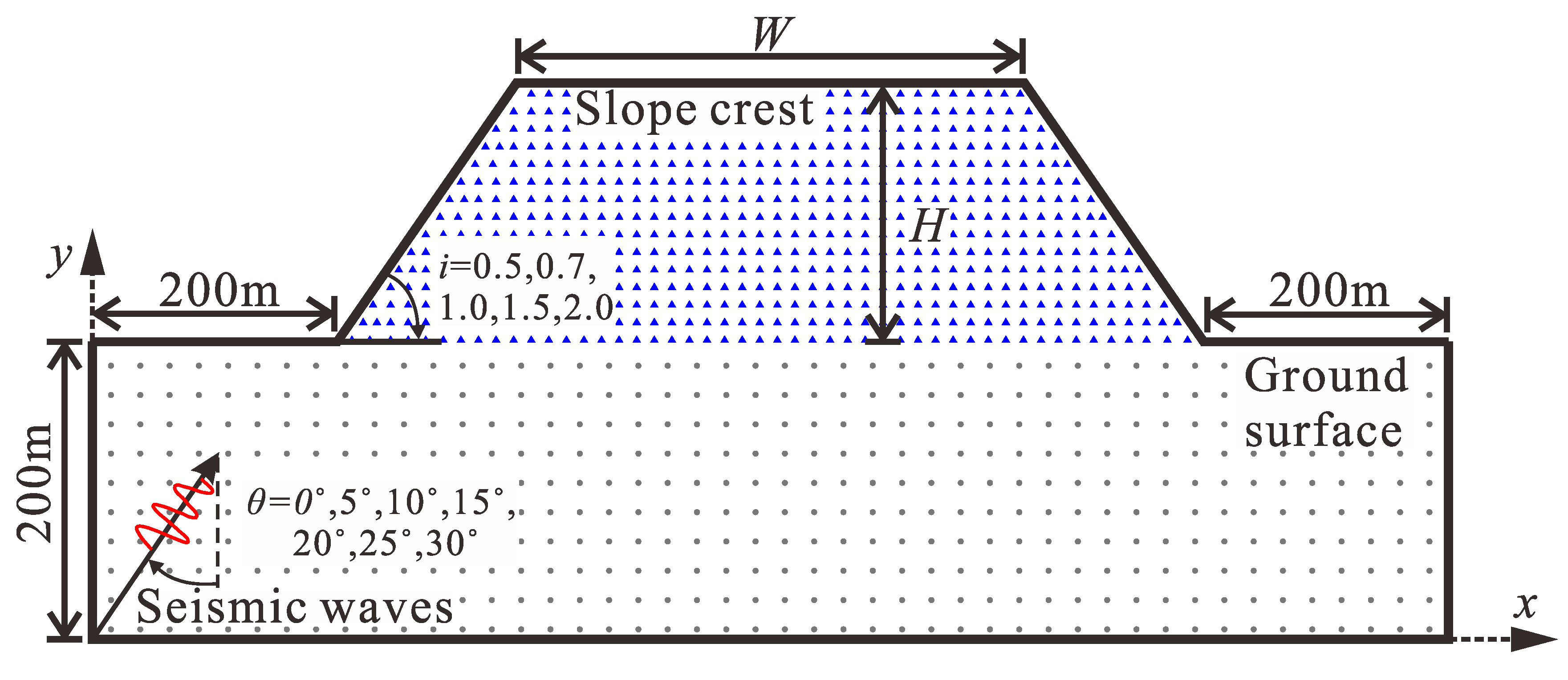
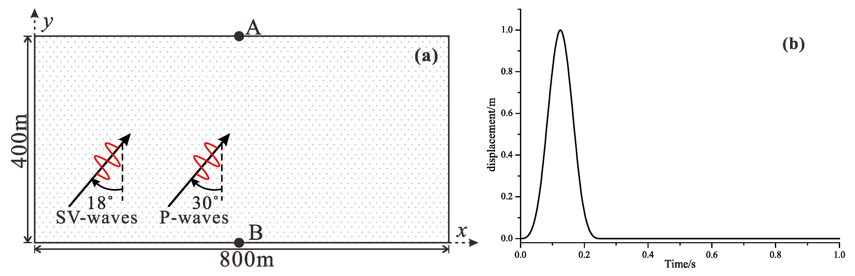
2. Problem Layout and Model Establishment
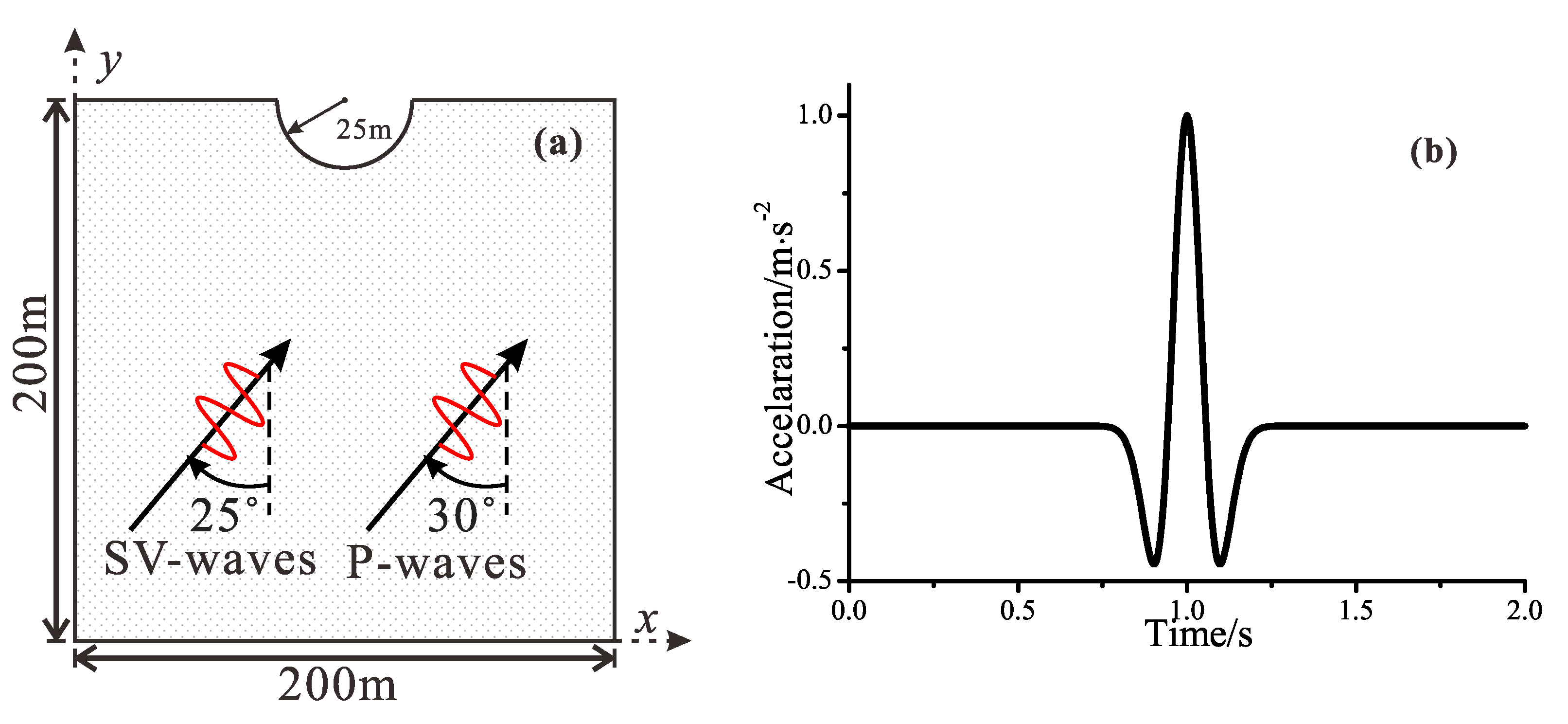
3. Input of Seismic Waves in Numerical Simulation
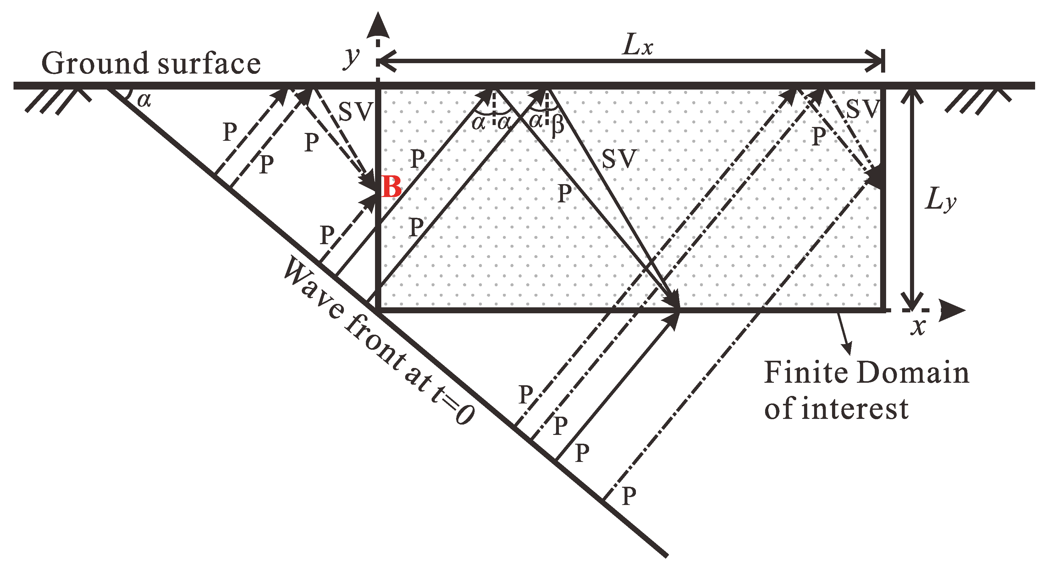
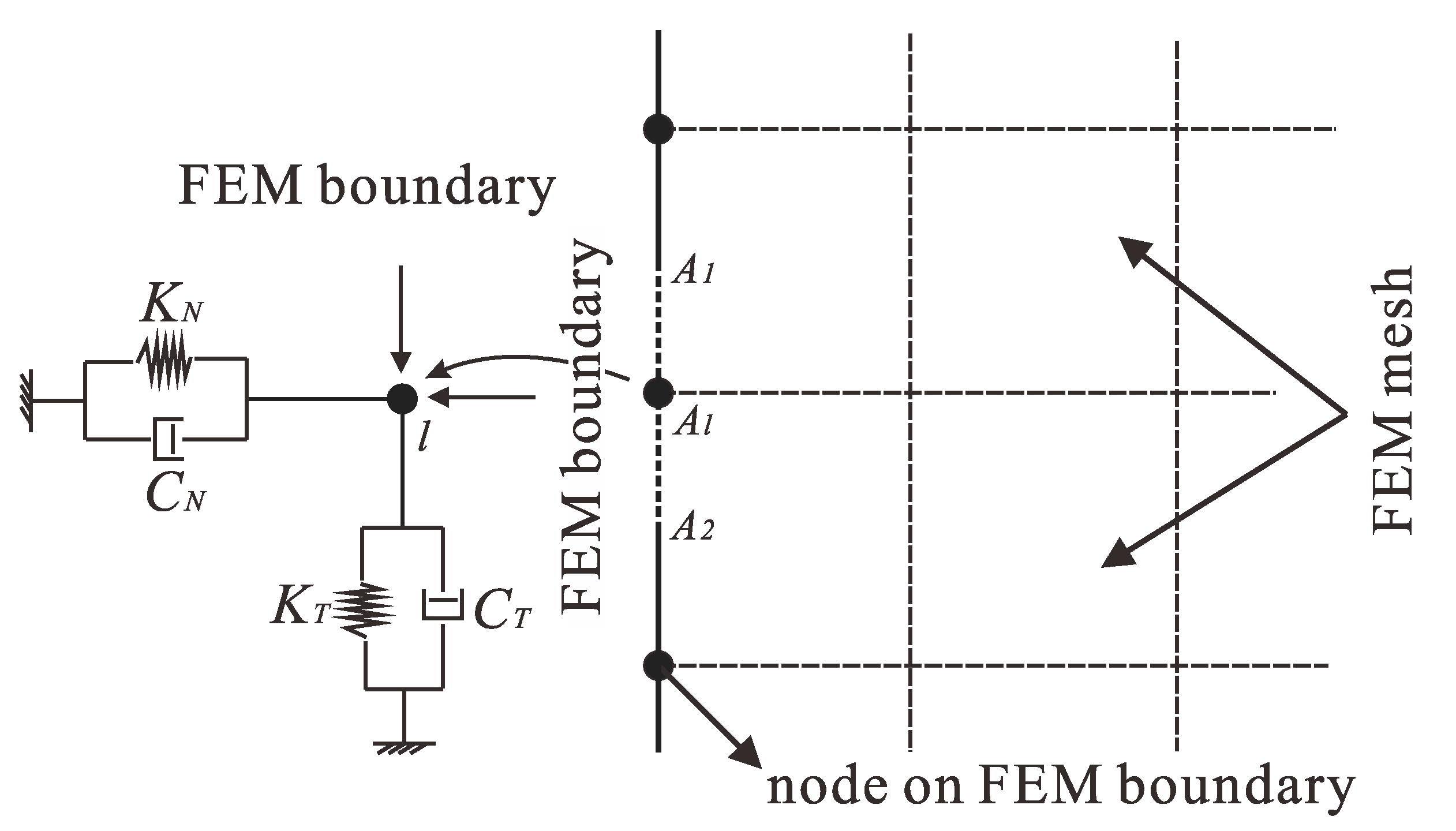
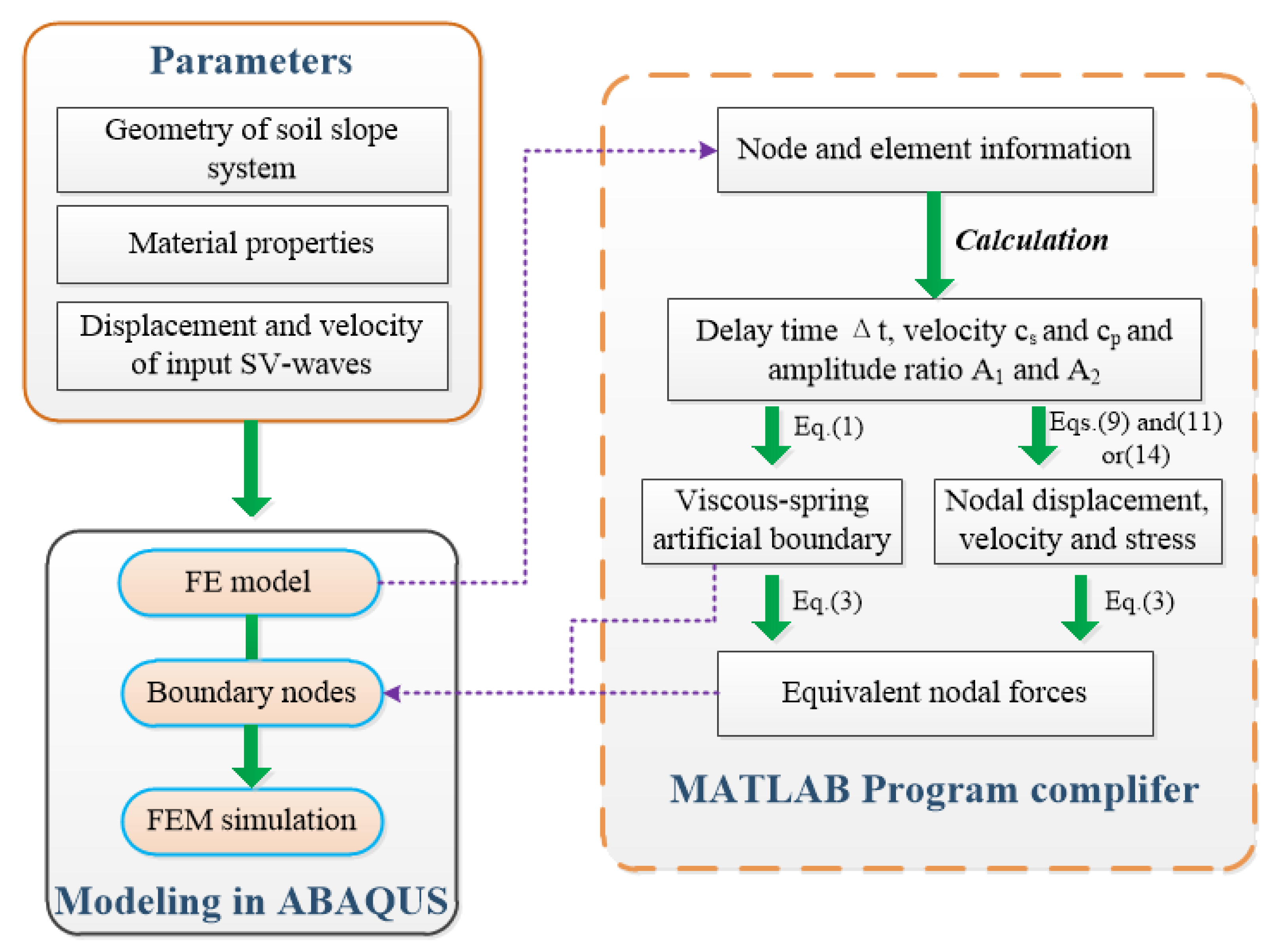
3.1. Establishment of the Artificial Boundary and the Input Method
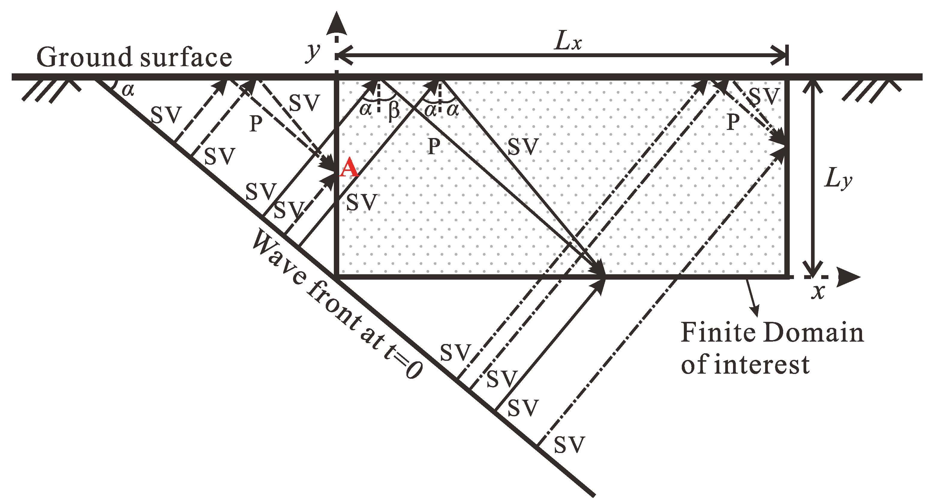
3.2. Implementation of Oblique Incident Waves
3.2.1. SV Waves
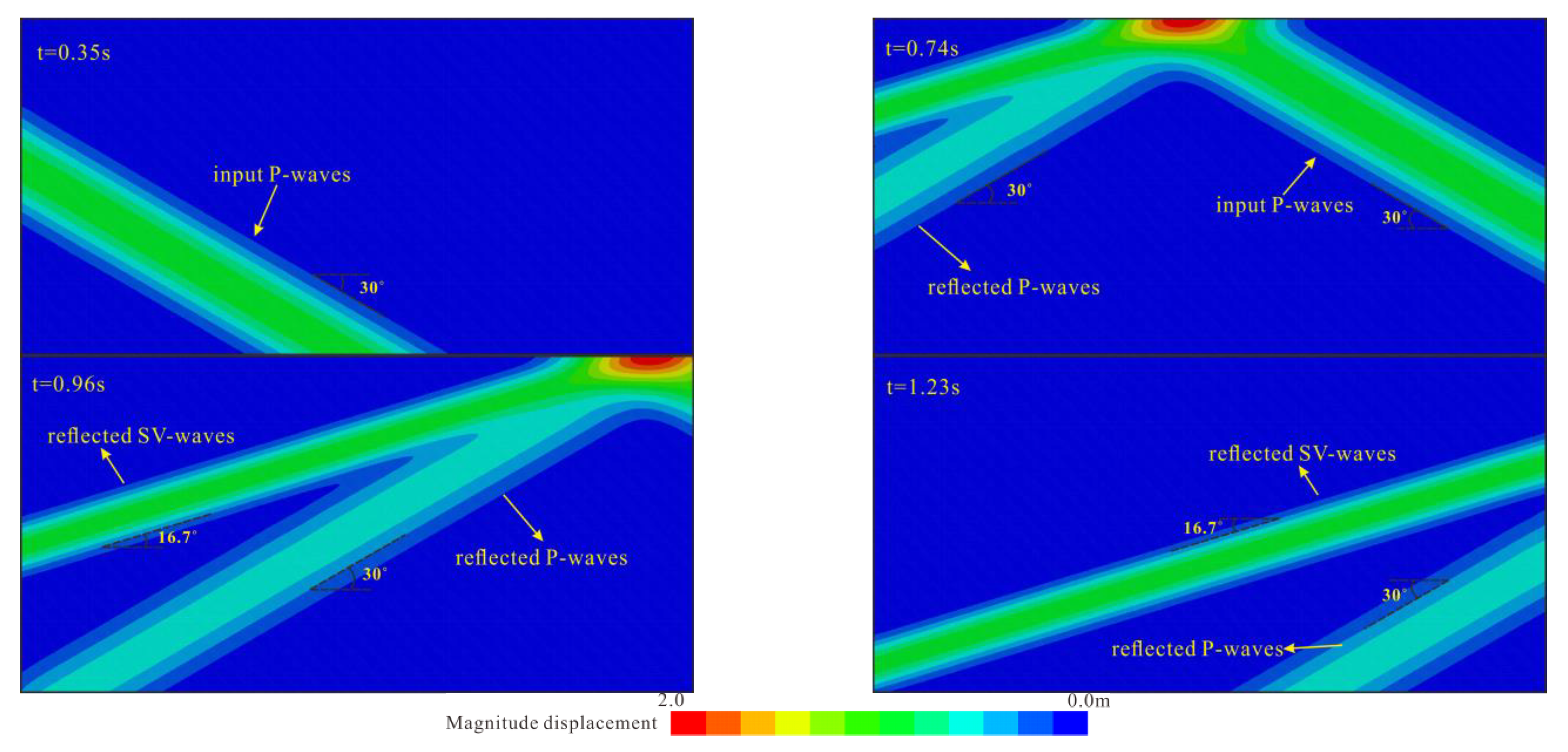
3.2.2. P Waves
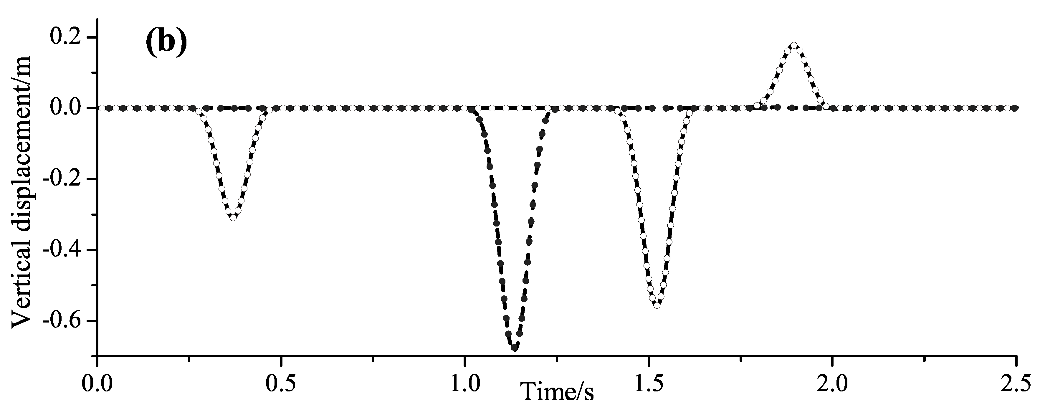
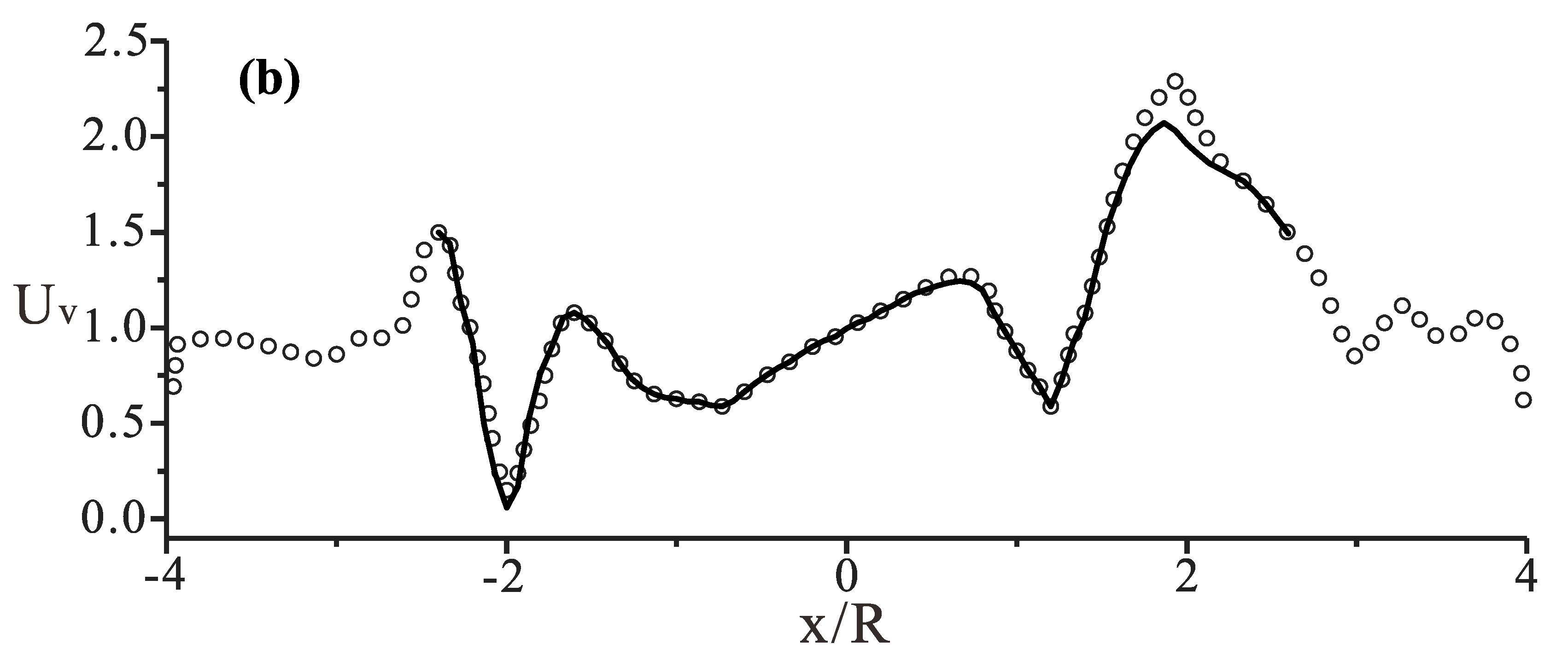
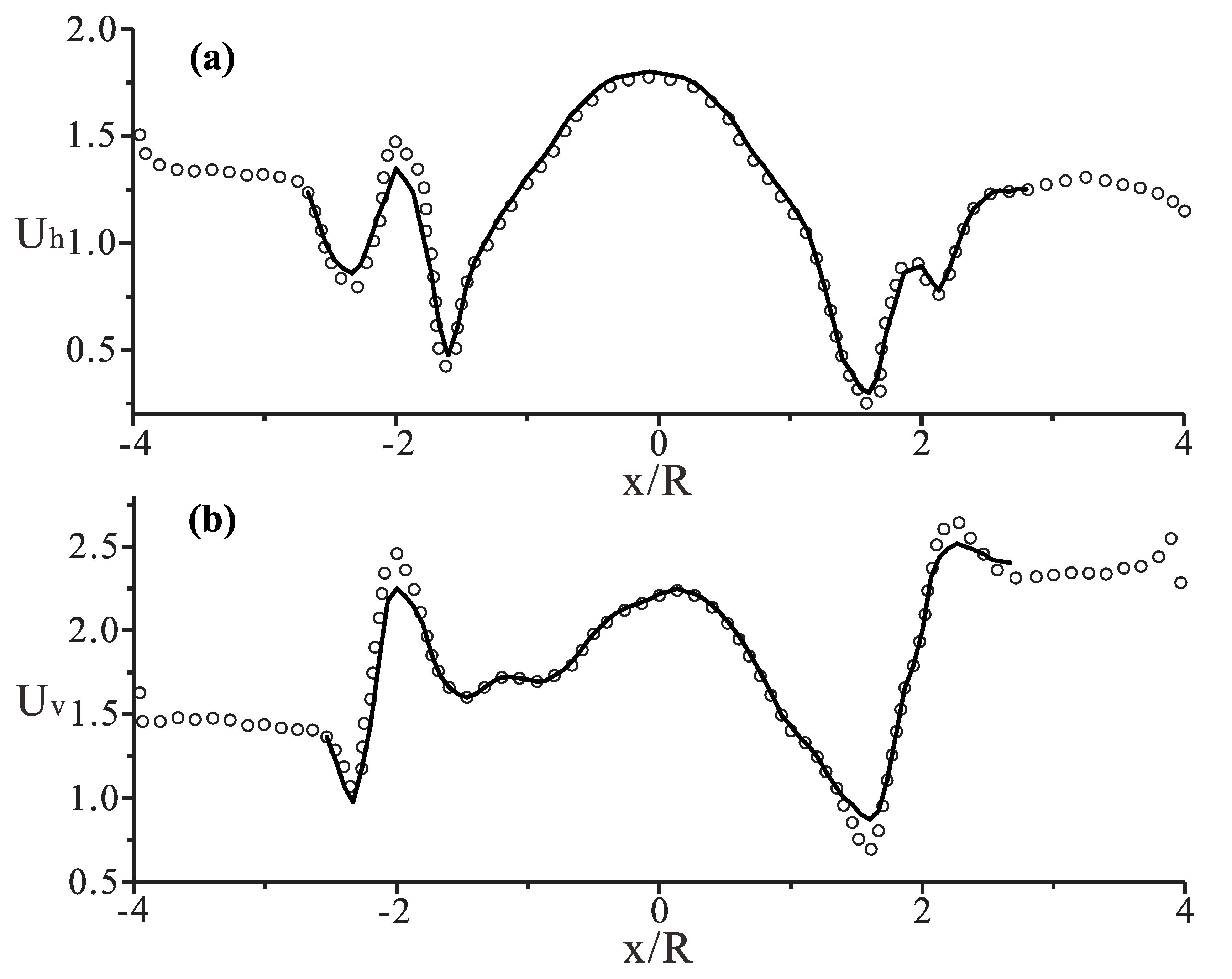
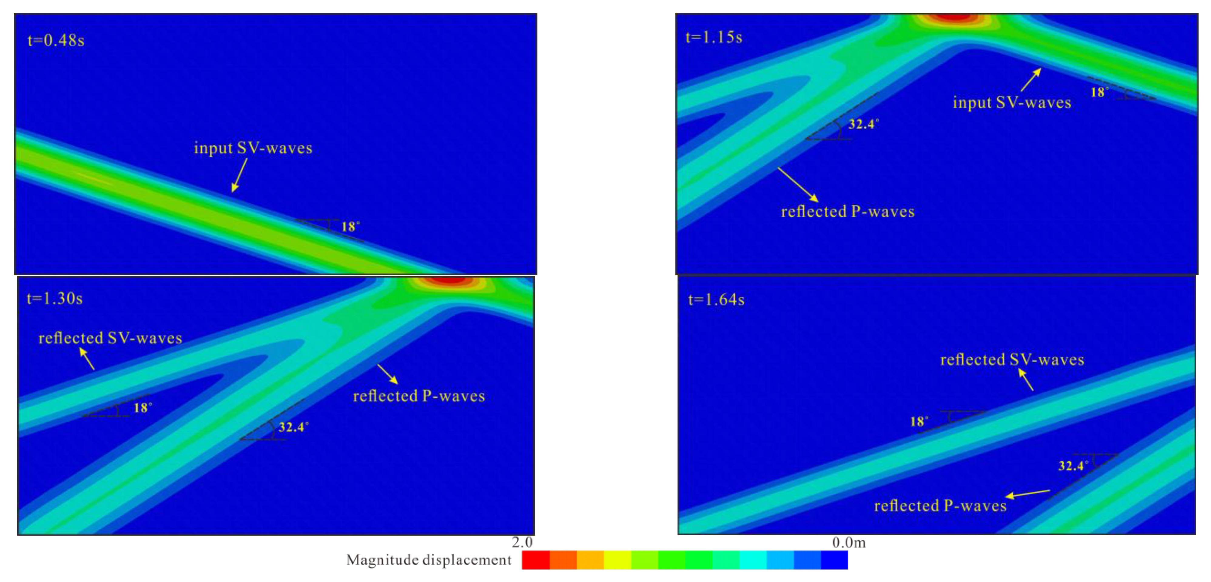
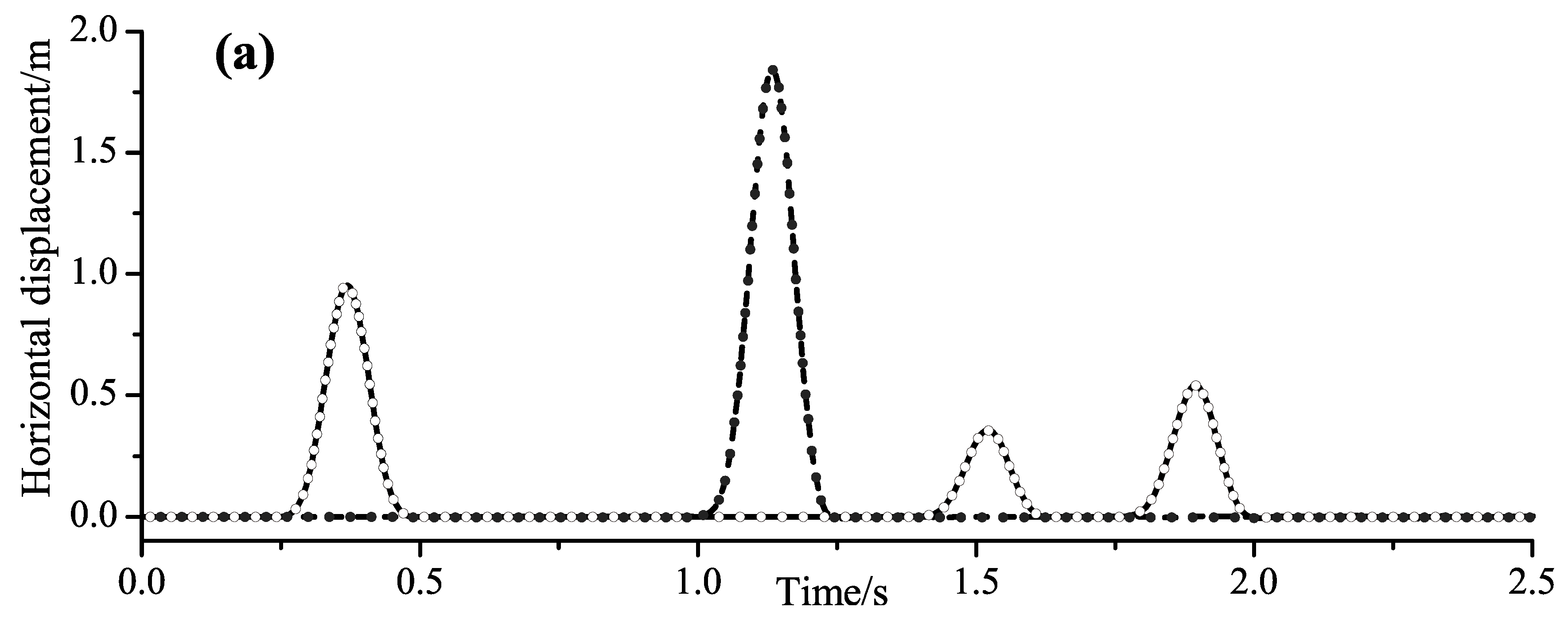
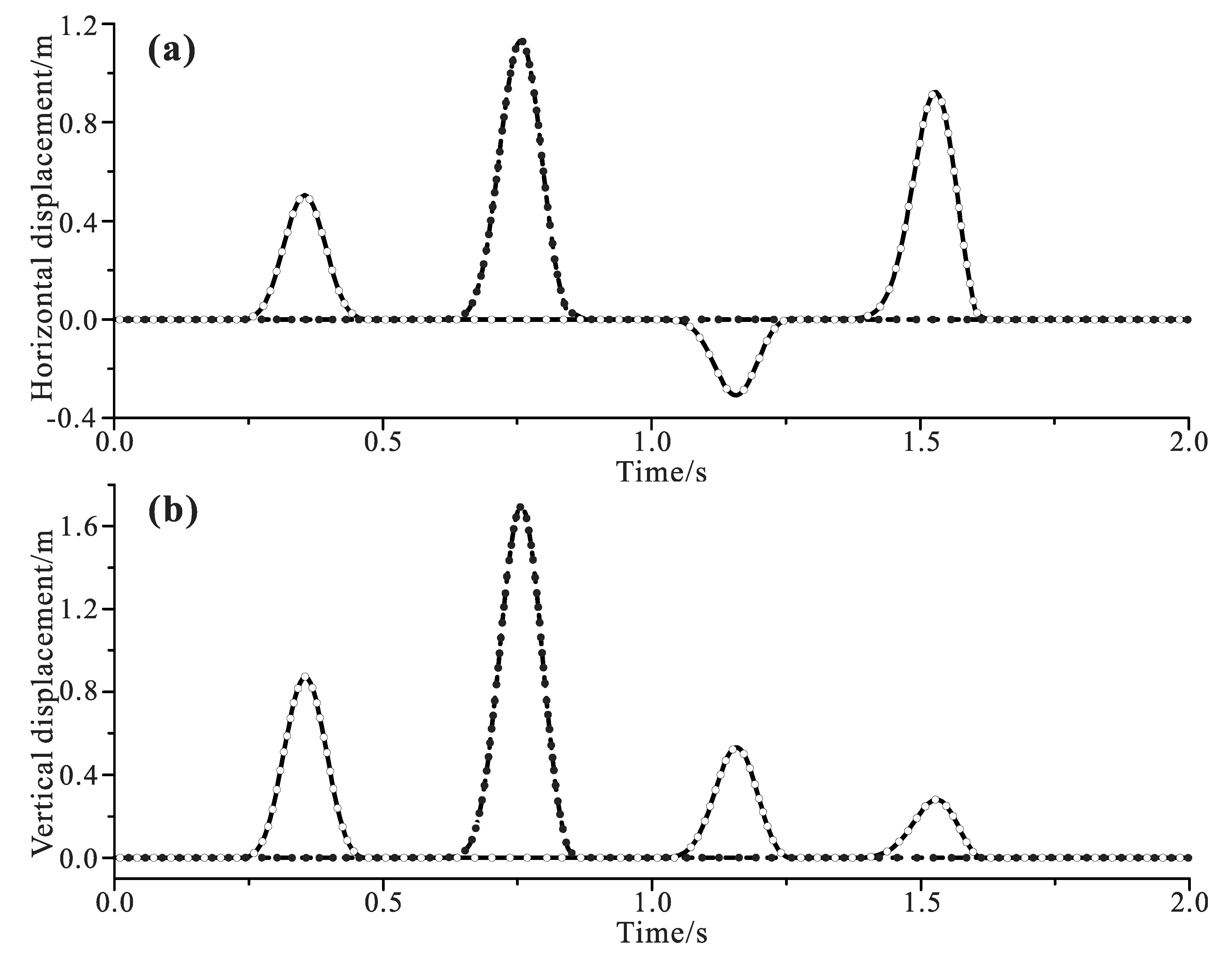
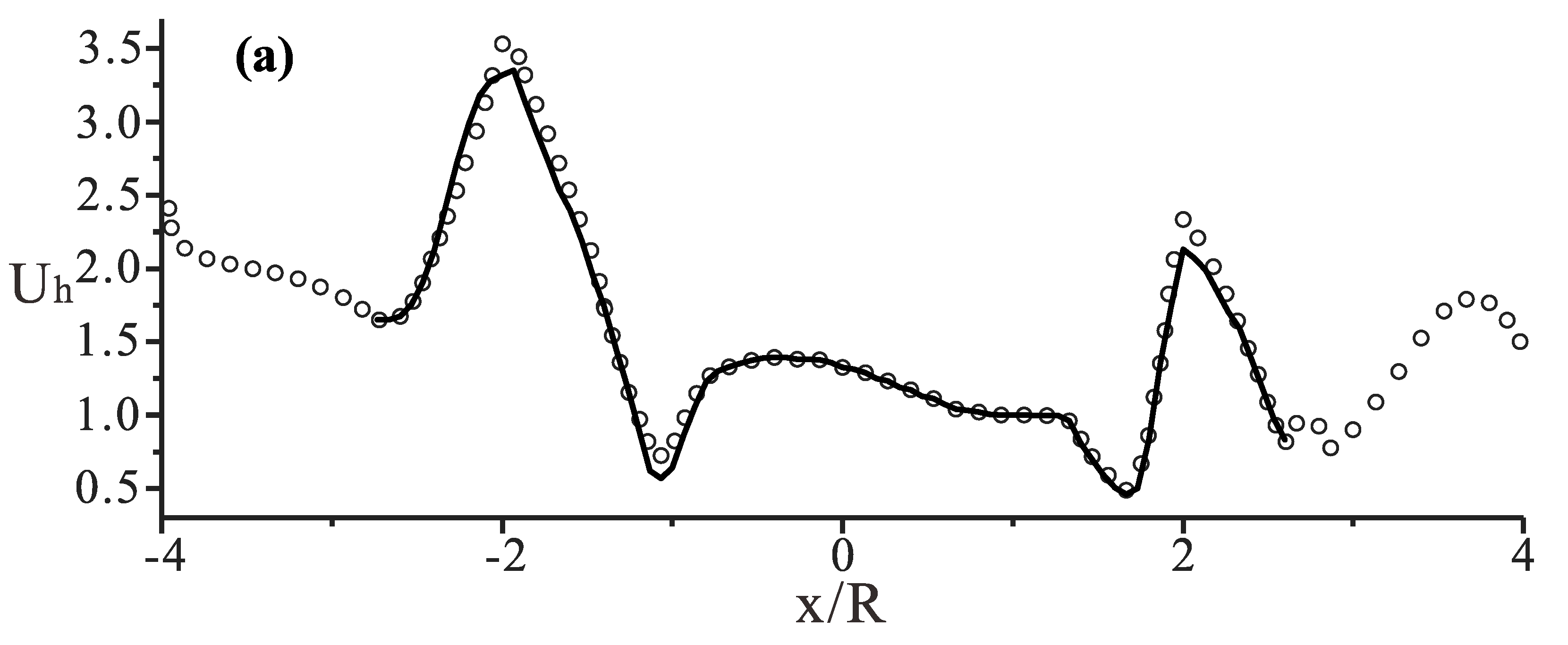
3.3. Verification
3.3.1. Test Example 1
3.3.2. Test Example 2
4. Discussion and Results
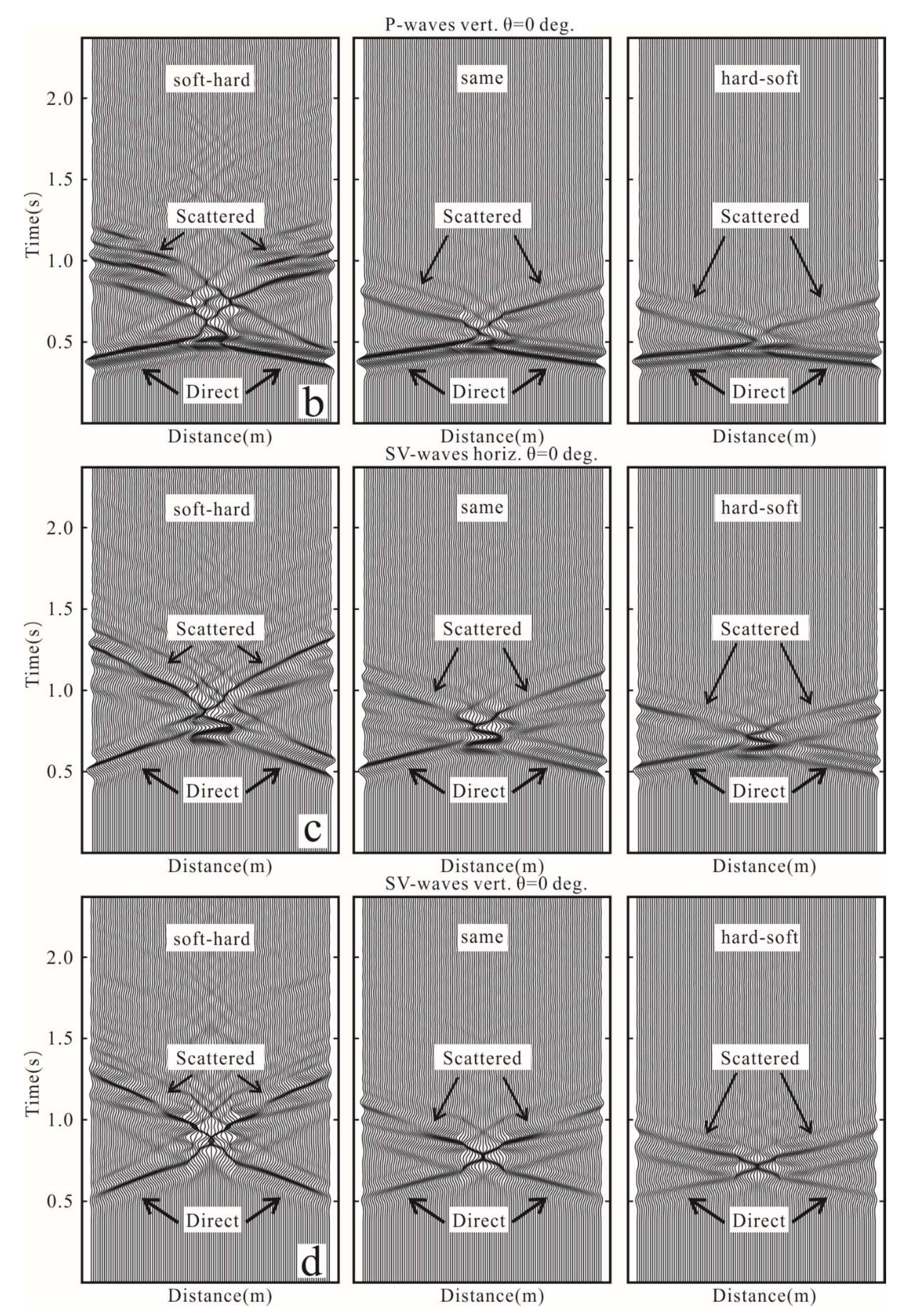
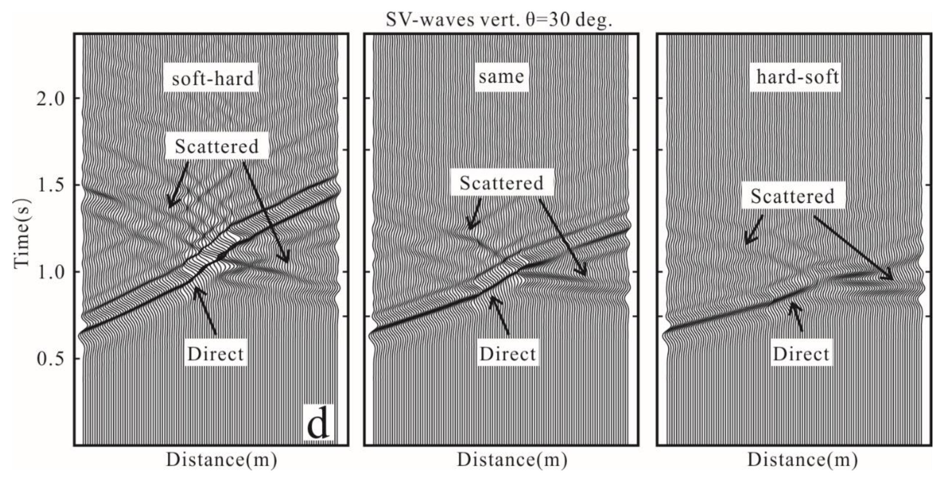
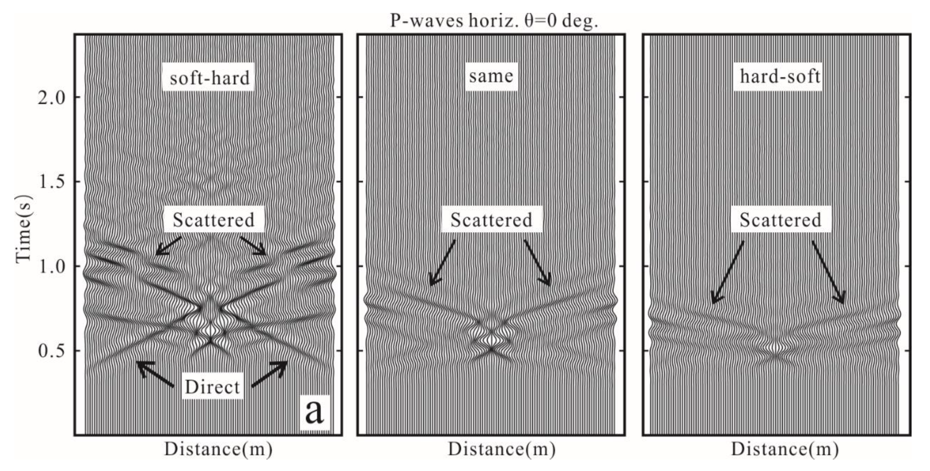
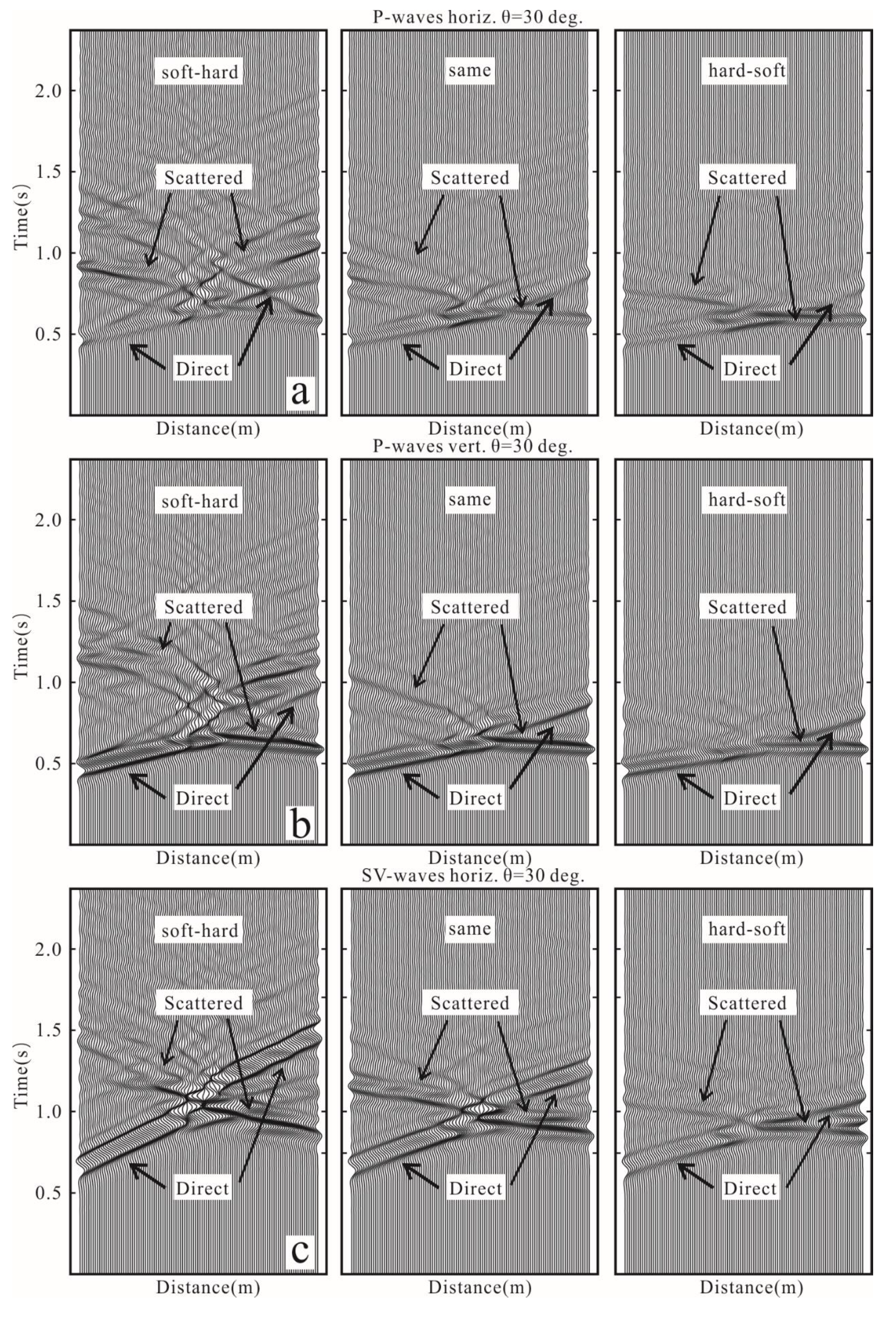
4.1. Effects of Wave Patterns
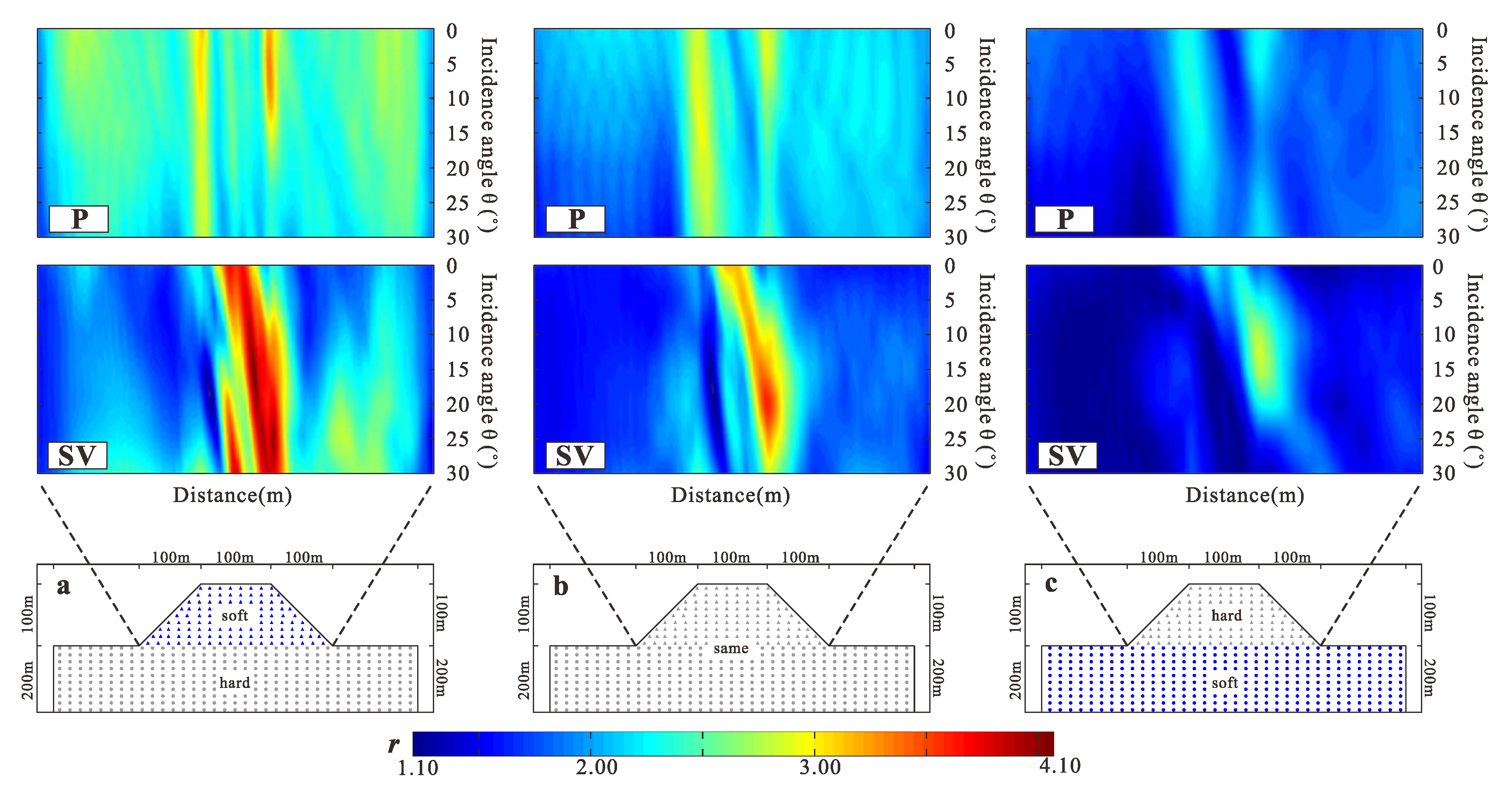
4.2. Effects of Materials
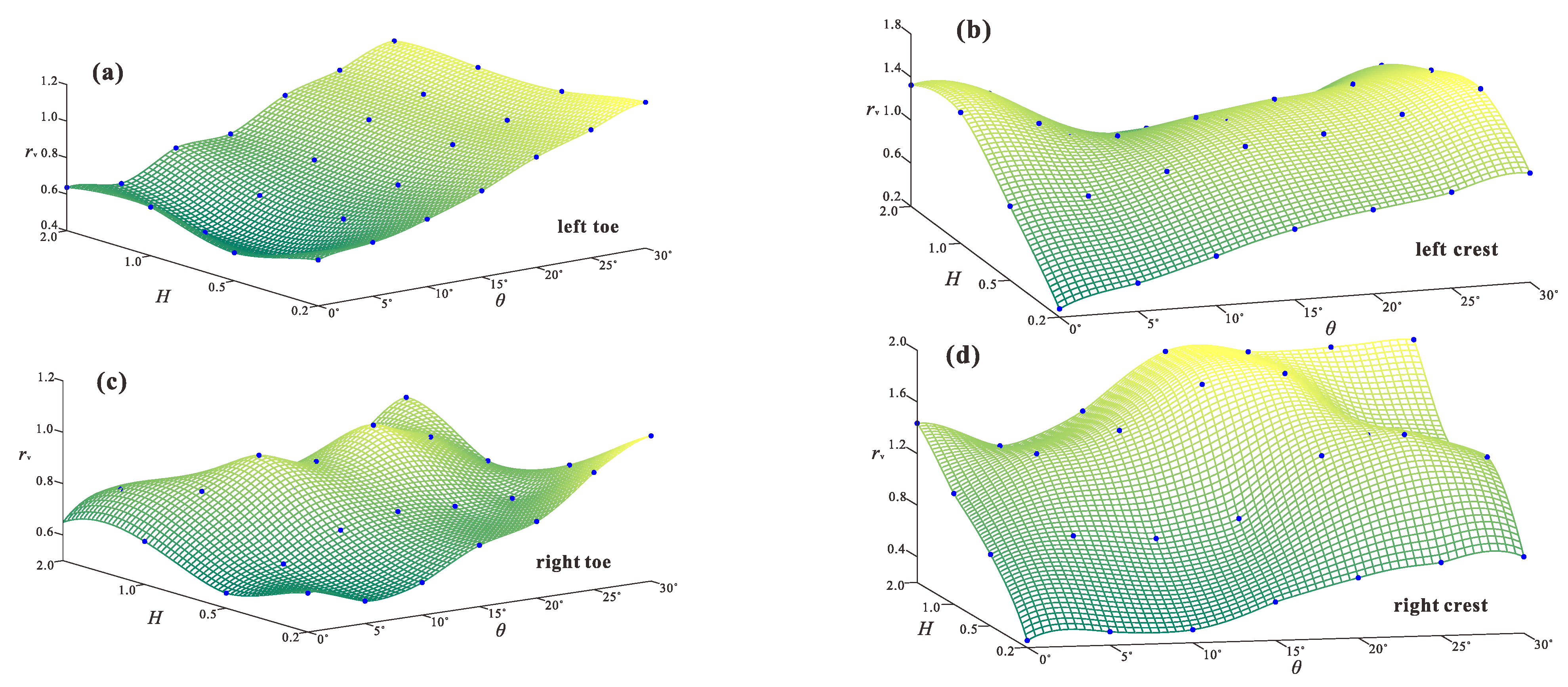
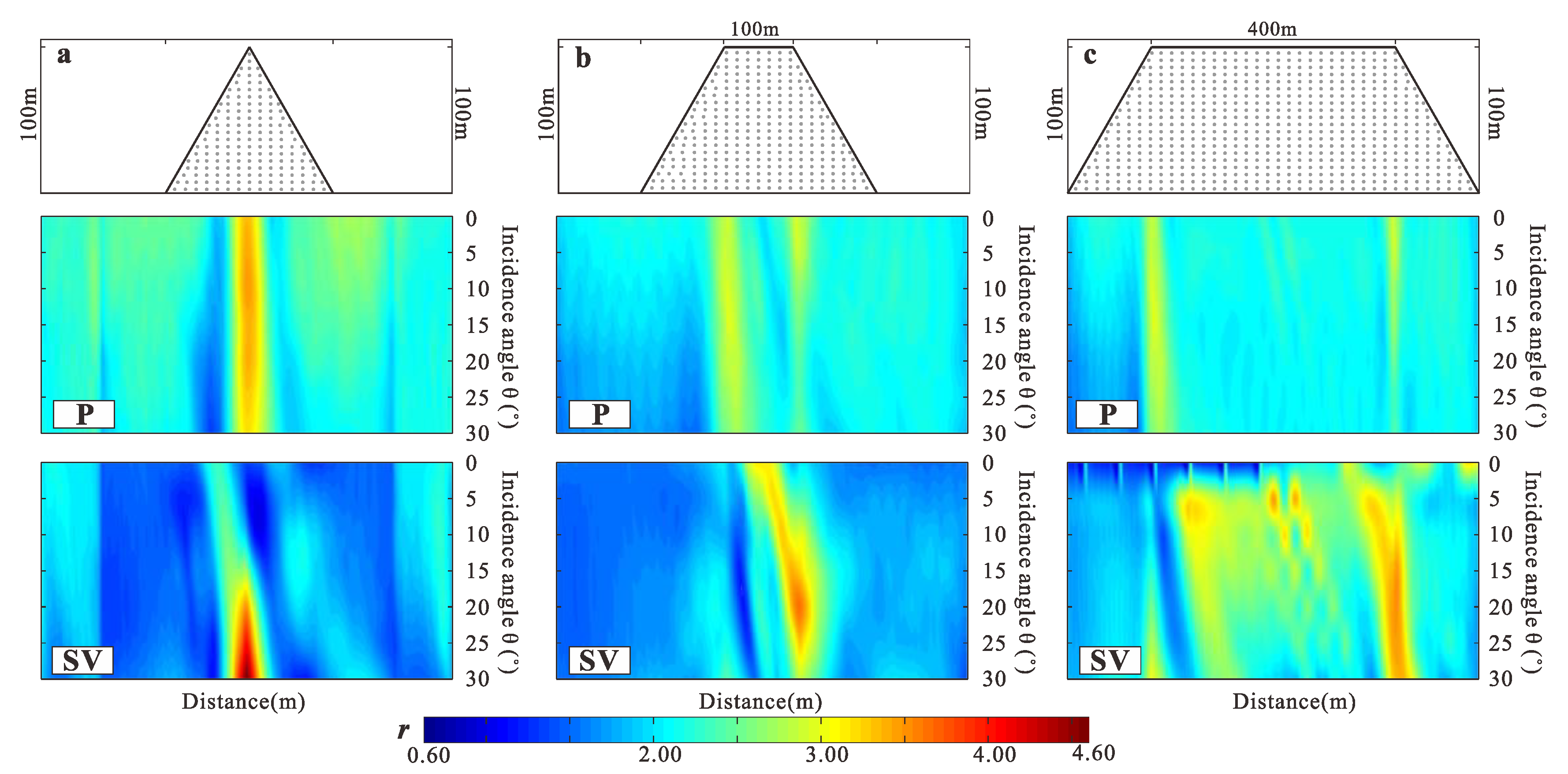
4.3. Effects of Slope Geometries
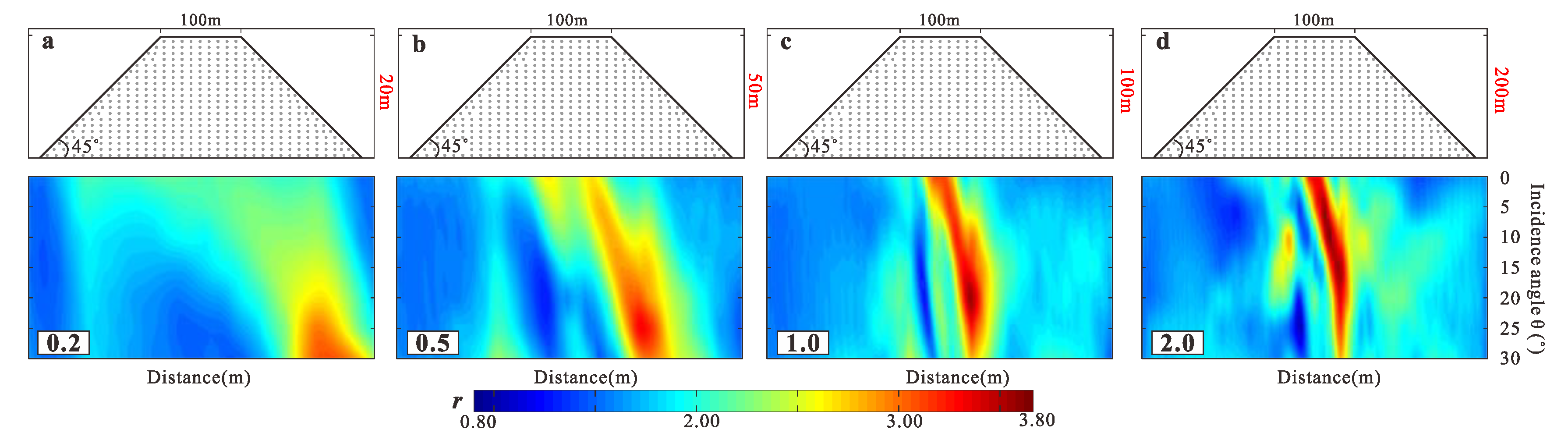
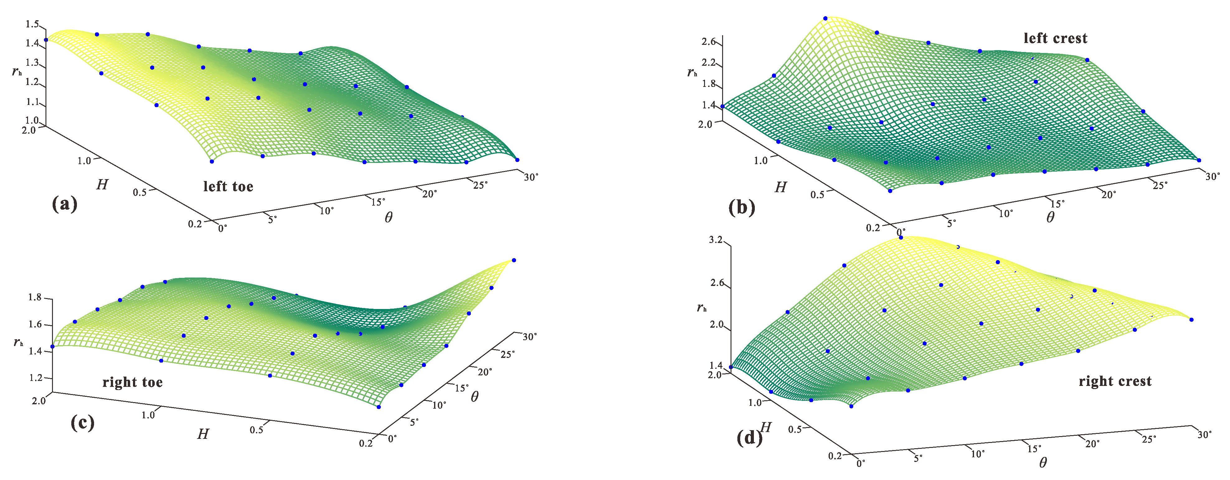
4.3.1. Influence of Slope Height H
4.3.2. Influence of the Width of Slope Crest W
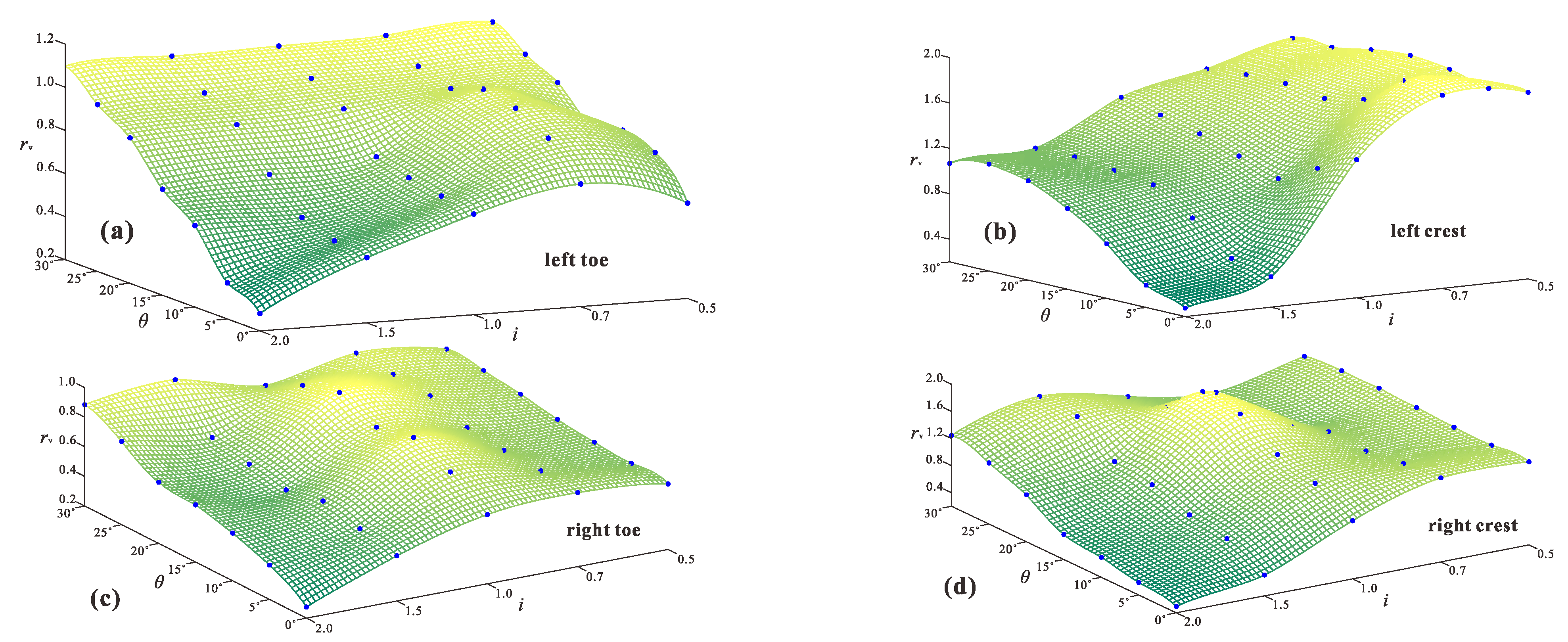
4.3.3. Influence of Slope Inclination I
5. Summary and Conclusions
Author Contributions
Funding
Institutional Review Board Statement
Informed Consent Statement
Data Availability Statement
Conflicts of Interest
References
- Alfaro, P.; Delgado, J.; García-Tortosa, F.J.; Lenti, L.; López, J.A.; López-Casado, C.; Martino, S. Widespread landslides induced by the Mw 5.1 earthquake of 11 May 2011 in Lorca, SE Spain. Eng. Geol. 2012, 137-138, 40–52. [Google Scholar] [CrossRef]
- Collins, B.D.; Kayen, R.; Tanaka, Y. Spatial distribution of landslides triggered from the 2007 Niigata Chuetsu–Oki Japan Earthquake. Eng. Geol. 2012, 127, 14–26. [Google Scholar] [CrossRef]
- Delgado, J.; García-Tortosa, F.J.; Garrido, J.; Loffredo, A.; López-Casado, C.; Martin-Rojas, I.; Rodríguez-Peces, M.J. Seismically-induced landslides by a low-magnitude earthquake: The Mw 4.7 Ossa De Montiel event (central Spain). Eng. Geol. 2015, 196, 280–285. [Google Scholar] [CrossRef] [Green Version]
- Tang, C.; Ma, G.C.; Chang, M.; Li, W.L.; Zhang, D.D.; Jia, T.; Zhou, Z.Y. Landslides triggered by the 20 April 2013 Lushan earthquake, Sichuan Province, China. Eng. Geol. 2015, 187, 45–55. [Google Scholar] [CrossRef]
- Wartman, J.; Dunham, L.; Tiwari, B.; Pradel, D. Landslides in eastern Honshu induced by the 2011 Tohoku earthquake. Bull. Seism. Soc. Am. 2013, 103, 1503–1521. [Google Scholar] [CrossRef]
- Xu, C.; Xu, X.W.; Shyu, J.B.H. Database and spatial distribution of landslides triggered by the Lushan, China Mw 6.6 earthquake of 20 April 2013. Geomorphology 2015, 248, 77–92. [Google Scholar] [CrossRef] [Green Version]
- Dunning, S.A.; Mitchell, W.A.; Rosser, N.J.; Petley, D.N. The Hattian Bala rock avalanche and associated landslides triggered by the Kashmir Earthquake of 8 October 2005. Eng. Geol. 2007, 93, 130–144. [Google Scholar] [CrossRef]
- Owen, L.A.; Kamp, U.; Khattak, G.A.; Harp, E.L.; Keefer, D.K.; Bauer, M.A. Landslides triggered by the 8 October 2005 Kashmir earthquake. Geomorphology 2008, 94, 1–9. [Google Scholar] [CrossRef]
- Yin, Y.P.; Wang, F.W.; Sun, P. Landslide hazards triggered by the 2008 Wenchuan earthquake, Sichuan, China. Landslides 2009, 6, 139–152. [Google Scholar] [CrossRef]
- Huang, R.; Pei, X.; Fan, X.; Zhang, W.; Li, S.; Li, B. The characteristics and failure mechanism of the largest landslide triggered by the Wenchuan earthquake, May 12, 2008, China. Landslides 2011, 9, 131–142. [Google Scholar] [CrossRef]
- Sepúlveda, S.A.; Murphy, W.; Jibson, R.W.; Petley, D.N. Seismically induced rock slope failures resulting from topographic amplification of strong ground motions: The case of Pacoima Canyon, California. Eng. Geol. 2005, 80, 336–348. [Google Scholar] [CrossRef]
- Sepúlveda, S.A.; Murphy, W.; Petley, D.N. Topographic controls on coseismic rock slides during the 1999 Chi-Chi earthquake, Taiwan. Q. J. Eng. Geol. Hydrogeol. 2005, 38, 189–196. [Google Scholar] [CrossRef]
- Bourdeau, C.; Havenith, H.B. Site effects modelling applied to the slope affected by the Suusamyr earthquake (Kyrgyzstan, 1992). Eng. Geol. 2008, 97, 126–145. [Google Scholar] [CrossRef]
- Bozzano, F.; Lenti, L.; Martino, S.; Paciello, A.; Mugnozza, G.S. Self-excitation process due to local seismic amplification responsible for the reactivation of the Salcito landslide (Italy) on 31 October 2002. J. Geophys. Res. Space Phys. 2008, 113, 1–21. [Google Scholar] [CrossRef] [Green Version]
- Del Gaudio, V.; Coccia, S.; Wasowski, J.; Gallipoli, M.R.; Mucciarelli, M. Detection of directivity in seismic site response from microtremor spectral analysis. Nat. Hazards Earth Syst. Sci. 2008, 8, 751–762. [Google Scholar] [CrossRef] [Green Version]
- Bozzano, F.; Lenti, L.; Martino, S.; Paciello, A.; Mugnozza, G.S. Evidences of landslide earthquake triggering due to self-excitation process. Int. J. Earth. Sci. 2011, 100, 861–879. [Google Scholar] [CrossRef]
- Lenti, L.; Martino, S. The interaction of seismic waves with step-like slopes and its influence on landslide movements. Eng. Geol. 2012, 126, 19–36. [Google Scholar] [CrossRef]
- Athanasopoulos, G.A.; Pelekis, P.C.; Leonidou, E.A. Effects of surface topography on seismic ground response in the Egion (Greece) 15 June 1995 earthquake. Soil. Dyn. Earthq. Eng. 1999, 18, 135–149. [Google Scholar] [CrossRef]
- Çelebi, M. Topographical and geological amplification: Case studies and engineering implications. Struct. Saf. 1991, 10, 199–217. [Google Scholar] [CrossRef]
- Wang, W.; Liu, B.D.; Liu, X.; Yang, M.L.; Zhou, Z.H. Analysis on the hill topography effect based on the strong ground motion records of Wenchuan Ms8.0 earthquake. Acta. Seismol. Sinica. 2015, 37, 452–462. [Google Scholar]
- Zaslavsky, Y.; Shapira, A. Experimental study of topographic amplification using the Israel seismic network. J. Earthq. Eng. 2000, 4, 43–65. [Google Scholar] [CrossRef]
- Bakavoli, M.K.; Haghshenas, E. Experimental and numerical study of topographic site effect on a hill near Tehran. In Proceedings of 5th International Conference on Recent Advances in Geotechnical Earthquake Engineering and Soil Dynamics, San Diego, CA, USA, 24 May 2010; pp. 1–10. [Google Scholar]
- Trifunac, M.D. Scattering of plane SH waves by a semi-cylindrical canyon. Earthq. Eng. Struct. Dyn. 1973, 1, 267–281. [Google Scholar] [CrossRef]
- Wong, H.L.; Trifunac, M.D. Scattering of plane SH waves by a semi-elliptical canyon. Earthq. Eng. Struct. Dyn. 1974, 3, 157–169. [Google Scholar] [CrossRef]
- Lee, V.W. Three-dimensional diffraction of plane P, SV & SH waves by a hemispherical alluvial valley. Soil Dyn. Earthq. Eng. 1984, 3, 133–144. [Google Scholar] [CrossRef]
- Lee, V.W. Scattering of plane SH-waves by a semi-parabolic cylindrical canyon in an elastic half-space. Geophys. J. Int. 1990, 100, 79–86. [Google Scholar] [CrossRef] [Green Version]
- Yuan, X.M.; Men, F.L. Scattering of plane SH waves by a semi-cylindrical hill. Earthq. Eng. Struct. Dyn. 1992, 21, 1091–1098. [Google Scholar] [CrossRef]
- Du, X.L.; Xiong, J.G.; Guan, H.M. Boundary integration equation method to scattering of plane SH-waves. Acta Seism. Sin. 1993, 6, 609–618. [Google Scholar] [CrossRef]
- Ashford, S.A.; Sitar, N. Analysis of topographic amplification of inclined shear waves in a steep coastal bluff. Bull. Seismol. Soc. Am. 1997, 87, 692–700. [Google Scholar] [CrossRef]
- Ashford, S.A.; Sitar, N.; Lysmer, J.; Deng, N. Topographic effects on the seismic response of steep slopes. Bull. Seism. Soc. Am. 1997, 87, 701–709. [Google Scholar]
- Han, F.; Wang, G.Z.; Kang, C.Y. Scattering of SH-waves on triangular hill joined by semi-cylindrical canyon. Appl. Math. Mech. 2011, 32, 309–326. [Google Scholar] [CrossRef]
- Yang, Z.L.; Xu, H.N. Ground motion of two scalene triangle hills and a semi-cylindrical canyon under incident SH-waves. Appl. Mech. Mater. 2012, 21–126, 862–866. [Google Scholar] [CrossRef]
- Lee, V.W.; Liu, W.Y. Two-dimensional scattering and diffraction of P- and SV-waves around a semi-circular canyon in an elastic half-space: An analytic solution via a stress-free wave function. Soil Dyn. Earthq. Eng. 2014, 63, 110–119. [Google Scholar] [CrossRef]
- Zhang, N.; Gao, Y.F.; Pak, R.Y.S. Soil and topographic effects on ground motion of a surficially inhomogeneous semi-cylindrical canyon under oblique incident SH waves. Soil. Dyn. Earthq. Eng. 2017, 95, 17–28. [Google Scholar] [CrossRef]
- Meunier, P.; Hovius, N.; Haines, J.A. Topographic site effects and the location of earthquake induced landslides. Earth Planet. Sci. Lett. 2008, 275, 221–232. [Google Scholar] [CrossRef]
- Bouckovalas, G.D.; Papadimitriou, A.G. Numerical evaluation of slope topography effects on seismic ground motion. Soil Dyn. Earthq. Eng. 2005, 25, 547–558. [Google Scholar] [CrossRef]
- Pagliaroli, A.; Lanzo, G.; Beniamino, E. Numerical evaluation of topographic effects at the nicastro ridge in Southern Italy. J. Earthq. Eng. 2011, 15, 404–432. [Google Scholar] [CrossRef]
- Narayan, J.P.; Kumar, V. Study of combined effects of sediment rheology and basement focusing in an unbounded viscoelastic medium using P-SV-Wave finite-difference modeling. Acta Geophys. 2014, 62, 1214–1245. [Google Scholar] [CrossRef]
- Hailemikael, S.; Lenti, L.; Martino, S.; Paciello, A.; Rossi, D.; Mugnozza, G.S. Ground-motion amplification at the Colle di Roio ridge, Central Italy: A combined effect of stratigraphy and topography. Geophys. J. Int. 2016, 206, 1–18. [Google Scholar] [CrossRef]
- Assimaki, D.; Gazetas, G.; Kausel, E. Effects of local soil conditions on the topographic aggravation of seismic motion: Parametric investigation and recorded field evidence from the 1999 Athens earthquake. Bull. Seism. Soc. Am. 2005, 95, 1059–1089. [Google Scholar] [CrossRef]
- Assimaki, D.; Kausel, E.; Gazetas, G. Wave propagation and soil structure interaction on a cliff crest during the 1999 Athens earthquake. Soil. Dyn. Earthq. Eng. 2005, 25, 513–527. [Google Scholar] [CrossRef]
- Lo Presti, D.C.F.; Lai, C.; Puci, I. ONDA: Computer code for nonlinear seismic response analyses of soil deposits. J. Geotech. Geoenviron. Eng. 2006, 132, 223–235. [Google Scholar] [CrossRef]
- Di Fiore, V. Seismic site amplification induced by topographic irregularity: Results of a numerical analysis on 2D synthetic models. Eng. Geol. 2010, 114, 109–115. [Google Scholar] [CrossRef]
- Tripe, R.; Kontoe, S.; Wong, T.K.C. Slope topography effects on ground motion in the presence of deep soil layers. Soil Dyn. Earthq. Eng. 2013, 50, 72–84. [Google Scholar] [CrossRef]
- Rizzitano, S.; Cascone, E.; Biondi, G. Coupling of topographic and stratigraphic effects on seismic response of slopes through 2D linear and equivalent linear analyses. Soil Dyn. Earthq. Eng. 2014, 67, 66–84. [Google Scholar] [CrossRef]
- Nguyen, K.V.; Gatmiri, B. Evaluation of seismic ground motion induced by topographic irregularity. Soil Dyn. Earthq. Eng. 2007, 27, 183–188. [Google Scholar] [CrossRef]
- Pagliaroli, A.; Avalle, A.; Falcucci, E.; Gori, S.; Galadini, F. Numerical and experimental evaluation of site effects at ridges characterized by complex geological setting. Bull. Earthq. Eng. 2015, 13, 2841–2865. [Google Scholar] [CrossRef]
- Gischig, V.S.; Eberhardt, E.; Moore, J.R.; Hungr, O. On the seismic response of deep-seated rock slope instabilities—Insights from numerical modeling. Eng. Geol. 2015, 193, 1–18. [Google Scholar] [CrossRef]
- Narayan, J.P.; Kumar, V. A numerical study of effects of ridge-weathering and ridge-shape-ratio on the ground motion characteristics. J. Seism. 2015, 19, 83–104. [Google Scholar] [CrossRef]
- Li, H.; Liu, Y.; Liu, L.; Liu, B.; Xia, X. Numerical evaluation of topographic effects on seismic response of single-faced rock slopes. Bull. Int. Assoc. Eng. Geol. Environ. 2017, 1873–1891. [Google Scholar] [CrossRef]
- Jin, X.; Liao, Z.P. Statistical research on S-wave incident angle. Earthq. Resear. Chin. 1994, 8, 121–131. [Google Scholar]
- Takahiro, S.; Kazuhiko, K.; Yoichi, S.; Dai, K.; Toru, M.; Ryoichi, T.; Chiaki, Y.; Takeshi, U. Estimation of earthquake motion incident angle at rock site. In Proceedings of the 12th World Conference Earthquake Engineering, NZ National Society for Earthquake Engineering, Auckland, New Zealand, 16 April 2000; pp. 1–8. [Google Scholar]
- Kuhlemeyer, R.L.; Lysmer, J. Finite element method accuracy for wave propagation problems. J. Soil Mech. Found. Div. 1973, 99, 421–427. [Google Scholar] [CrossRef]
- Deeks, A.J.; Randolph, M.F. Axisymmetric time-domain transmitting boundaries. J. Eng. Mech. 1994, 120, 25–42. [Google Scholar] [CrossRef]
- Liu, J.B.; Lv, Y.D. A direct method for analysis of dynamic soil-structure interaction based on interface idea. Chin. Civ. Eng. J. 1998, 83, 261–276. [Google Scholar] [CrossRef]
- Du, X.L.; Zhao, M.; Wang, J.T. A stress artificial boundary in FEA for near-field wave problem. Chin. J. Theor. Appl. Mech. 2006, 38, 49–56. [Google Scholar]
- Yin, C.; Li, W.H.; Zhao, C.G.; Kong, X.A. Impact of tensile strength and incident angles on a soil slope under earthquake SV-waves. Eng. Geol. 2019, 260, 1–11. [Google Scholar] [CrossRef]
- Eringen, A.C.; Suhubi, E.S. Elastodynamics; Academic Press: New York, NY, USA, 1975. [Google Scholar]
- Ewing, W.M.; Jardetzky, W.S.; Press, F.; Beiser, A. Elastic Waves in Layered Media; McGraw-Hill: New York, NY, USA, 1957. [Google Scholar]
- Wong, H.L. Effect of surface topography on the diffraction of P, SV, and Rayleigh waves. Bull. Seismol. Soc. Am. 1982, 72, 1167–1183. [Google Scholar]
- Lenti, L.; Martino, S. A parametric numerical study of the interaction between seismic waves and Landslides for the evaluation of the susceptibility to seismically induced displacements. Bull. Seismol. Soc. Am. 2013, 103, 33–56. [Google Scholar] [CrossRef]


| Soil Types | Mass Density (kg/m3) | Poison’s Ratio | Elastic Modulus E (MPa) | P Wave Velocity cp (m/s) | S Wave Velocity cs (m/s) |
|---|---|---|---|---|---|
| Foundation | 2000 | 0.2 | 768 | 653.1 | 400 |
| Slope I | 2000 | 0.2 | 768 | 653.1 | 400 |
| Slope II | 2000 | 0.3 | 425 | 534.8 | 285.9 |
| Slope III | 2000 | 0.25 | 1370 | 906.4 | 523.4 |
Publisher’s Note: MDPI stays neutral with regard to jurisdictional claims in published maps and institutional affiliations. |
© 2021 by the authors. Licensee MDPI, Basel, Switzerland. This article is an open access article distributed under the terms and conditions of the Creative Commons Attribution (CC BY) license (https://creativecommons.org/licenses/by/4.0/).
Share and Cite
Yin, C.; Li, W.-H.; Wang, W. Evaluation of Ground Motion Amplification Effects in Slope Topography Induced by the Arbitrary Directions of Seismic Waves. Energies 2021, 14, 6744. https://doi.org/10.3390/en14206744
Yin C, Li W-H, Wang W. Evaluation of Ground Motion Amplification Effects in Slope Topography Induced by the Arbitrary Directions of Seismic Waves. Energies. 2021; 14(20):6744. https://doi.org/10.3390/en14206744
Chicago/Turabian StyleYin, Chao, Wei-Hua Li, and Wei Wang. 2021. "Evaluation of Ground Motion Amplification Effects in Slope Topography Induced by the Arbitrary Directions of Seismic Waves" Energies 14, no. 20: 6744. https://doi.org/10.3390/en14206744
APA StyleYin, C., Li, W.-H., & Wang, W. (2021). Evaluation of Ground Motion Amplification Effects in Slope Topography Induced by the Arbitrary Directions of Seismic Waves. Energies, 14(20), 6744. https://doi.org/10.3390/en14206744