Article

Impact of Charging Electric Vehicles under Different State of Charge Levels and Extreme Conditions

1
Canada Excellence Research Chair Team, Concordia University, Montreal, QC H3G 1M8, Canada
2
Department of Electrical Engineering, Faculty of Technology, University of Batna 2, Fesdis, Batna 05078, Algeria
3
Electrical and Computer Engineering Department, Miami University, 260Q Garland Hall, 650 East High Street, Oxford, OH 45056, USA
4
School of Engineering Technology, College of the North Atlantic, Al Tarafa, Jelaiah Street, Duhail North, Doha P.O. Box 24449, Qatar
*
Author to whom correspondence should be addressed.
Energies 2021, 14(20), 6589; https://doi.org/10.3390/en14206589
Submission received: 24 September 2021 / Revised: 9 October 2021 / Accepted: 11 October 2021 / Published: 13 October 2021
(This article belongs to the Special Issue Electric Vehicle Charging Networks)

Abstract

:
High penetration levels of Plug-in Electric Vehicles (PEVs) could cause stress on the network and might violate the limits and constraints under extreme conditions, such as exceeding power and voltage limits on transformers and power lines. This paper defines extreme conditions as the state of a load or network that breaks the limits of the constraints in an optimization model. Once these constraints are violated, the optimization algorithm might not work correctly and might not converge to a feasible solution, especially when the complexity of the system increases and includes nonlinearities. Hence, the algorithm may not help in mitigating the impact of penetrating PEVs under extreme conditions. To solve this problem, an original algorithm is suggested that is able to adapt the constraints’ limits according to the energy demand and the energy needed to charge the PEVs. Different case scenarios are studied for validation purposes, such as charging PEVs under different state of charge levels, different energy demands at home, and different pricing mechanisms. Results show that our original algorithm improved the profiles of the voltage and power under extreme conditions. Hence, the algorithm is able to improve the integration of a high number of PEVs on the distribution system under extreme conditions while preserving its stability.

1. Introduction

1.1. Motivation and Background

The future of the transportation sector relies heavily on the deployment of a high number of plug-in electric vehicles (PEVs) in smart cities and districts [1,2,3]. Since PEVs depend only on electricity to work, they need battery storage systems (BSSs) to store and deliver energy to the vehicles. The main problem of BSSs is that their energy density is lower than conventional fuel [4]. Therefore, the size of a BSS is much bigger than a fuel tank since the only way to charge the battery is by connecting it to the electricity network. Hence, high demand might be created on the network during a short period of time (e.g., 19.2 kW @ level 2) [5,6,7]. Moreover, the car owner may not need to fully charge his PEV for a certain trip; maybe 60% or 80% is enough. Some questions come to mind as follows. Is it necessary to fully charge the battery for a certain trip? What will be the impact of charging the battery to 80% instead of 100% on the network? What will happen if there are power and energy limits in which PEVs cannot fully charge or can only charge to a certain desired State of Charge (SOC) level? All these questions motivated us to write this paper.

1.2. Literature Review

In recent years, PEVs have become a hot topic, especially when it comes to their impact on the distribution network [8,9,10]. Many papers have developed algorithms to schedule their charging at the home level [11,12,13], while others have studied their scheduling in parking lots [14,15], and charging stations [16,17]. In [18], authors developed a sophisticated algorithm to foresee the final desired SOC for a specific journey considering many factors such as distance, road conditions, etc. The estimation of the final SOC at the destination allows the car owner to know how much energy is needed for the trip and how much the initial SOC should be. The findings were interesting; however, the techno-economic impact of considering different State of Charge levels on the distribution systems was not considered. Many attempts have been made to study the impact of the high penetration level of PEVs on the network [19,20,21,22]. For instance, high power demand may perturb the voltage stability on the network [23,24,25], and sophisticated algorithms are needed to mitigate the impact of PEVs during peak periods [26,27,28,29]. However, it is not known what the impact will be when considering different SOC levels and not just the penetration level of PEVs. In addition, to the best of the authors’ knowledge, studying the optimal scheduling of PEVs under extreme conditions has not been done yet. In this paper, extreme conditions can be defined as the state of a load or network that breaks the limits of the constraints in an optimization model. However, such constraints are highly dependent on a specific application and the optimization model. If the constraints are physical ones, such as the circuit breaker limit at home (e.g., 32 A @ 230 V, or ≈7.4 kW), any violation of these constraints will result in activating protection devices such as tripping the circuit breaker in order to avoid any overload. Therefore, the optimization process will stop working correctly since the physical constraints are violated. On the other hand, if non-physical constraints are violated (such as a virtual power limit which is lower than the real circuit breaker limit, e.g., 5 kW < 7.4 kW), in this case, the physical system works; however, some perturbation might happen to the optimization process, and it might not give optimal results or solutions. Therefore, the power losses might increase, and the electricity price might not be minimized. For example, if the constraint of the maximum energy demand on a particular transformer is 1 MWh/day, an energy demand of 1.5 MWh/day is considered an extreme condition in which the constraints of the optimization model are not satisfied. Hence, there is a high possibility that the algorithm will not converge to an optimal solution. Therefore, there is a high risk that the optimal scheduling of PEVs may not be correct or precise. Consequently, the PEVs tend to charge during peak demand which will worsen the situation of the network. From this place, it is important to propose an algorithm that takes into account all these anomalies or extreme conditions in the optimization model. Hence, the algorithm will be capable of detecting the anomalies and modifying some parameters in the optimization model in order to avoid any constraint violations, either physical or non-physical.

1.3. Contributions

This paper tries to answer the previously mentioned questions and solve the highlighted problems. To do so, the contributions in this paper are presented as follows:
  • A novel optimization algorithm is proposed to schedule the charging of EVs under extreme conditions. Hence, the problem of divergence is solved.
  • The impact of different SOC levels at home is studied. The main goal is to show how much the final SOC affects the techno-economic aspects at home and answer the question of whether it is necessary to fully charge PEVs or not.
For validation purposes, different scenarios are considered: (a) three pricing mechanisms are considered, which are flat price, time-of-use (TOU), and dynamic price; (b) two SOC levels are studied and compared, 80% and 100%; (c) the impact on the power and voltage profiles is studied; (d) power losses, voltage drop, and line currents are calculated.

1.4. Paper Organization

The problem formulation is presented in Section 2, including the optimization model and algorithm. Section 3 shows the results for a single home. Finally, the conclusion is presented in Section 4.

2. Problem Formulation

The mathematical equations of the optimization model are presented. In addition, an algorithm is proposed to eliminate the divergence from the simulation and always find solutions under extreme conditions. However, before going deeper into the mathematical modeling, it is important to mention why the desired final SOC was chosen to be studied for this paper. What are the advantages and disadvantages of fully charging the battery, and what is the impact on the voltage drop and power losses?

2.1. Advantages and Disadvantages of Fully Charging the PEV

Many papers have considered that the final SOC of a PEV should be equal to the unity (SOC = 1 or 100%) [30,31,32,33], while PEV owners may not need this level for a certain trip and a lower SOC level could be enough. Full charging can be resumed later at the destination point or even on the way, which will reduce the stress on the network in peak hours. A fully charged EV can have some advantages and disadvantages, as will be discussed in this subsection. It is important to mention that the initial SOC should be considered. Therefore, in this paper, the term used to describe the energy needed to charge the PEV to a certain State of Charge level is called “desired SOC level” ( SOC D ), which is equal to the difference between the final and initial SOC as in Equation (1). Hence, a fully charged EV is not the reference since the initial SOC can be 95%, and the final is 100%, in which 5% might not have any impact on the network. In addition, the energy should be considered since 5% in a small battery is not the same for a larger battery.
SOC D = SOC f SOC i
The advantages of a high SOC D can be presented as follows:
  • The traveling distance becomes longer,
  • Less range anxiety of the car owner,
  • The lifetime of the battery is increased in case the charging power rate is low.
On the other side, a high SOC D may have disadvantages and can cause many problems, such as:
  • Increasing the stress on the battery in case a high-power rate is used for charging,
  • Increasing the charging power rate, which will increase the internal temperature of the battery, thus reducing its lifetime.
  • Increasing the stress on the network, buses, parking lot, charging station, or even at home, in which the scheduling becomes more compressed and complicated, causing the charging of PEVs to occur during an on-peak time, or even creating peak demand during an off-peak time, therefore creating many problems on the network, such as voltage deviation and high peak demand.
  • Creating a high peak demand, which may cause severe problems to the transformer, such as overheating and overloading, and may cause it to disconnect and reduce its lifetime.
  • In case the electricity price is variable, the charging may occur during high electricity price times; thus, an unnecessary additional cost will be charged to the PEV owner. The remaining amount of energy could be charged later when the electricity price is low.

2.2. Advantages of the Desired SOC Level

To solve the problems mentioned in the previous subsection, this paper defines the desired SOC level ( SOC D ) as the needed SOC for a particular trip without the necessity to fully charge the PEV. SOC D has many advantages, as follows:
  • Decreases the stress on the energy storage system, such as the battery, during the charging process in which the charging power rates become lower, causing less tear on the battery,
  • Allows more PEVs to take part in the charging process in parking lots,
  • Reduces the life loss of the battery caused by high charging rates,
  • Reduces the charging cost of PEV, in which an algorithm shifts the charging of PEV to a later period when the electricity price is lower,
  • Reduces the time of charging of a single PEV,
  • Reduces the stress on the network and parking lots caused by the high charging demand,
  • The charging process of the PEV better respects the restraints and limits enforced by the parking lot, transformer, and bus and the charging power rates respect these constraints. Charging during the on-peak time is reduced, and there is no new peak during an off-peak time.
  • If the time for charging the battery to the desired level is not enough, the charging power rate is increased until the SOC D is satisfied.

2.3. Optimization Model

The objective function of the optimization model is presented in Equation (2). It schedules the charging power rate of a PEV in the presence of a baseload at home. Where C t Elec is the electricity price at instant t during the period T . Three electricity prices were chosen in this paper, namely fixed cost (or flat rate), time-of-use (TOU), and dynamic price. P t BL is the home’s baseload power profile, which cannot be controlled. P t PEV is the power demand of the PEV, which is controlled in the optimization process. Δ t is the time interval for simulation purposes (e.g., Δ t = 0.5   h ) .
ObjFun = Minimize   t T C t Elec · P t BL + P t PEV · Δ t
Equations (3)–(7) presents the constraints of the optimization model. Where Equation (3) shows the maximum power limit ( P t Max ) at home that should not be exceeded, including the baseload ( P t BL ) and the charging power of the PEV ( P t PEV ); η c is the charging efficiency of the battery; P t Max is described in Equation (4); P MCB represents the main circuit breaker power rating (e.g., 6.4 kW ≈ 32 A × 230 V, for cos(φ) = 1); P t RL is the reference power limit determined by the Distribution System Operator (DSO) or the distribution aggregator on the network (e.g., P t RL = 8   kW at t = 3 h, and P t RL = 9   kW at t = 5 h); P t RL is used in order to increase or decrease the power consumption at home, which is highly dependent on the requirements of the distribution system operator or the distribution aggregator. For instance, any excess of power demands on the transformer might reduce its lifetime drastically; therefore, the system operator may decrease P t RL for a specific period. As a consequence, the power demand of all consumers on the same transformer will be eventually reduced in order to maintain the stability of the network, or at least to minimize the losses and the damages that might occur due to the high power demand of the end-users. On the other hand, the system operator may increase P t RL limit when needed, which allows end-users to increase their electricity consumption during a certain period, which might support the network to maintain its stability and a balance between power generation and consumption. Equation (5) shows the minimum ( B Cap SOC Min ) and maximum ( B Cap SOC D ) energy limits of the battery, respectively. B Cap is the capacity of the battery (i.e., B Cap = 100   kWh ). Equation (6) represents the home’s energy demand limit for a specific time interval T i T located between the minimum ( E T i Min ) and maximum ( E T i Max ) limits. Finally, the minimum discharging limit ( P t Min   Disch ) and the maximum charging limit ( P t Max   Ch ) at instant “t” of the PEVs are presented in Equation (7).
P t BL + P t PEV η c P t Max
P t Max = min P MCB ,   P t RL
B Cap SOC Min t T P t PEV Δ t B Cap SOC D
E T i Min t T i P t BL + P t PEV Δ t E T i Max
P t Min   Disch P t PEV P t Max   Ch

2.4. Proposed Algorithm

In the previous section the optimization model was proposed, which schedules the charging of the PEV based on the electricity price while respecting the power limit P t Max . However, the optimization fails to work correctly if at least one of the constraints is violated, especially Equation (3). The violation could happen when the car’s owner wants to charge his PEV to a higher SOC level (e.g., 100%) within a very short period of time (e.g., 1 h), especially when there is already a peak demand at home. In this case, the optimization might not give accurate scheduling since the solution does not converge. From this place, it is important to create an algorithm that updates and changes the value of some parameters in the optimization model in order to get a feasible solution. To do so, the algorithm in Figure 1 is proposed to solve the problem of divergence while respecting the constraints. The first step is to collect data from the user, system operator, and PEV. Then, the algorithm calculates the needed energy to charge the battery ( E needed PEV ), and the maximum power limit ( P t Max ). Then, the algorithm calculates the available energy at home in period T , which is not used. Afterward, the algorithm compares the available energy to the needed energy to charge the battery. In case the first one is lower, the algorithm asks the user if he can reduce the desired SOC level; if not, the algorithm modifies the limit of the reference limit ( P t RL ) until E av E needed PEV . Next, the algorithm starts the optimization, and if the final SOC is less than the desired SOC level, the algorithm increases the charging power rate until the SOC D is attained.
Usually, there are two types of constraints, physical (such as circuit breaker limits, e.g., 32 A @ 230 V, or ≈7.4 kW), and non-physical (such as a virtual power limit which is lower than the real circuit breaker limit, e.g., 5 kW < 7.4 kW). Violating physical constraints may result in the interruption or failure of the system or by activating protection devices such as tripping the circuit breaker in order to avoid any overload. In this case, any violation in the physical constraints may stop the system and deactivate the optimization process. On the other hand, violating non-physical constraints may result in some perturbation in the optimization process. It is always possible to obtain results; however, they might not be the best ones or the optimal ones. In some cases, the algorithm might diverge, and results become worse than without optimization. From this place, introducing the reference limit ( P t RL ), as in Equation (8), will modify the constraint in Equation (4) in a way to increase the power limit at home and allow the PEV to have enough energy to charge its battery to the desired level. In this way, constraint violations become less probable, which will allow the optimization model to find the best or the optimal solution.
P t RL P t RL α + 1 ,   α > 0
On the other hand, if there is enough available energy to charge the PEV to the desired level and the charging power limit might not be high enough to satisfy the needs of the PEV, in this case the algorithm increases the maximum charging power limit ( P t Max   Ch ) as in Equation (9). The increase in P t Max   Ch limit will allow the PEV to charge its battery with a higher power rate. Therefore, the desired SOC level can be attained in a shorter period without violating the constraints of the optimization model.
P t Max   Ch P t Max   Ch β + 1 ,   β > 0

3. Results and Discussion

3.1. Assumptions

  • In this paper, two case studies are considered. The first one considers that the available energy in period T is enough to charge the PEV to the desired SOC level at home. In the second case, the available energy at home in period T is insufficient to charge the PEV to the desired State of Charge level.
  • Two different SOC levels are considered for each case, 80% and 100%.
  • Three different pricing mechanisms are considered for each case, as presented in Figure 2.
  • MATLAB is considered to solve the presented optimization model, which is regarded as a Mixed Integer Linear Programming (MILP) problem since the objective function and constraints are convex and global optimal solution can achieved. The solver used in MATLAB is “intlinprog”.
  • Voltage drops, power losses, and profiles are presented for each case scenario.

3.2. Case 1: Charging Time Is Enough to Charge the PEV to the Desired State of Charge Level

In this subsection, the charging time is considered large enough to charge the PEV to the desired SOC level. Two different SOC levels are studied for the same period of time. SOC D = 1 , and SOC D = 0.8 , in which the rest of the energy (1 − 0.8 = 0.2) is charged later when the PEV arrives at the destination, on the way, or when it comes back home. 
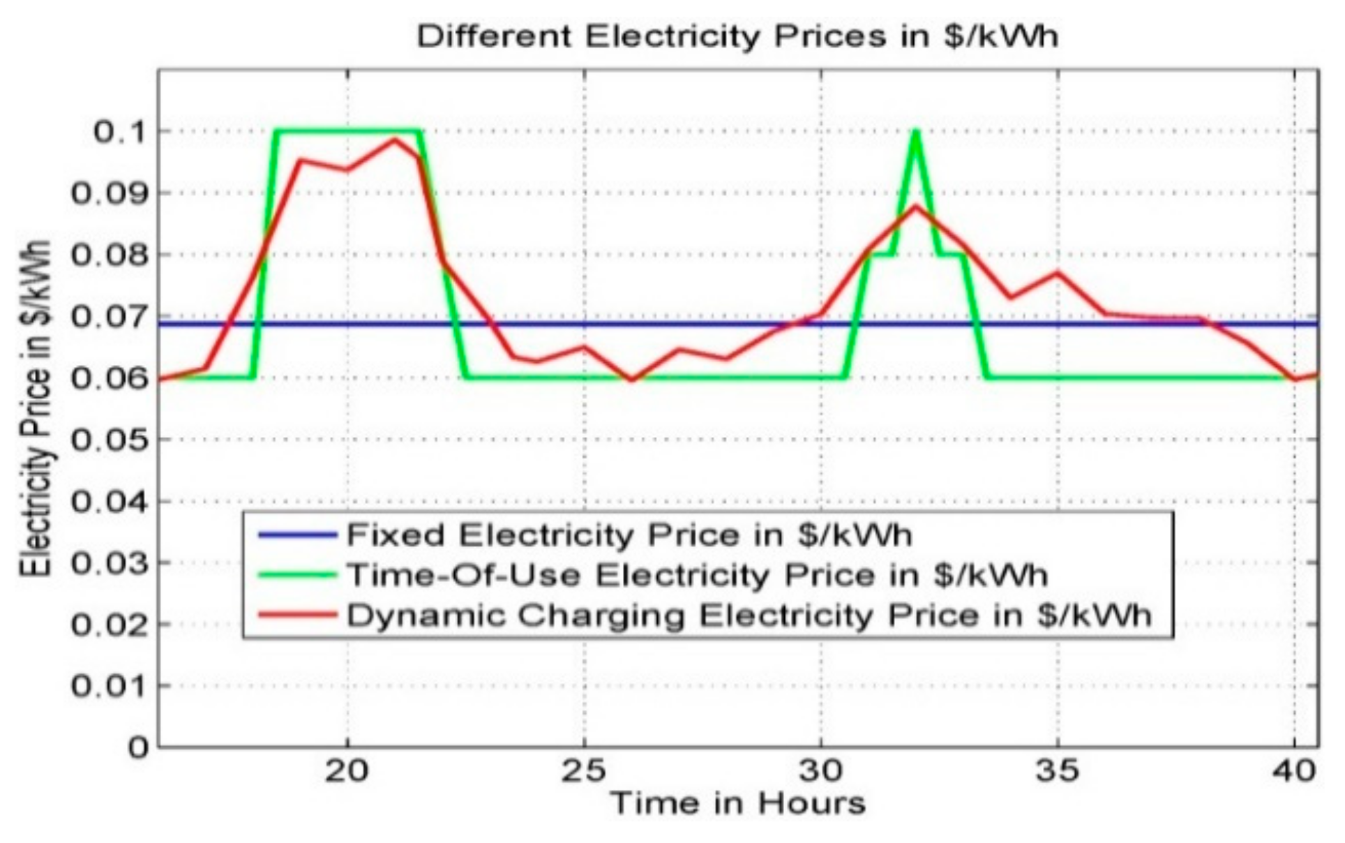
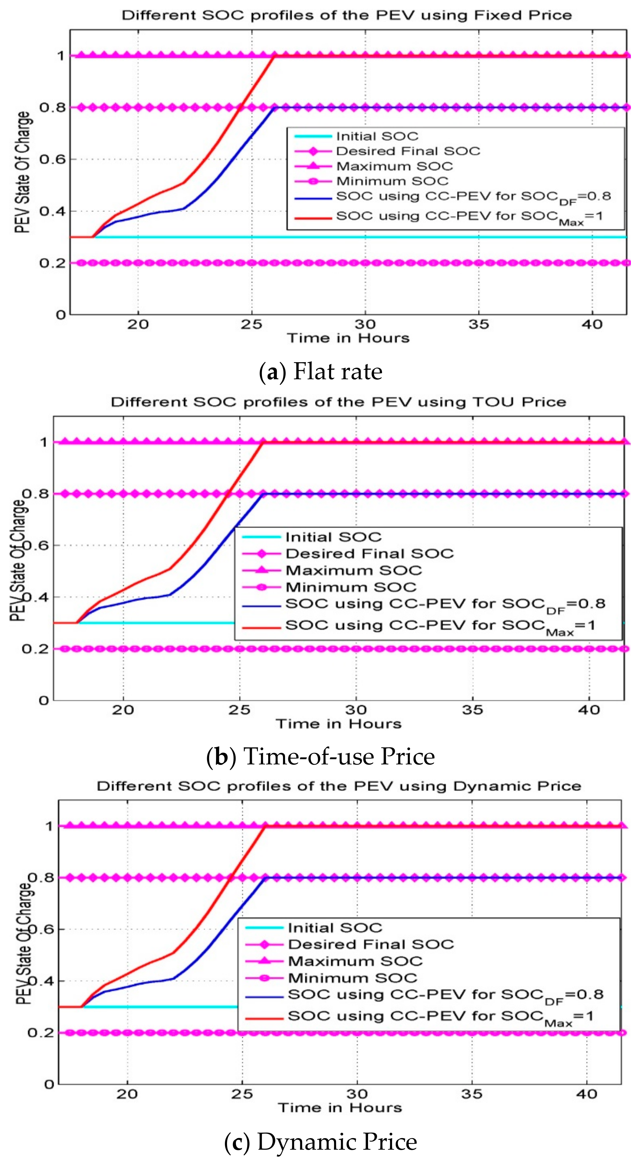
Figure 3 shows the SOC profile under three different pricing mechanisms and for two SOC levels. It can be remarked how much the electricity price affects the SOC profile during the charging process. In addition, the car owner is satisfied because the final SOC level is equal to the desired one.
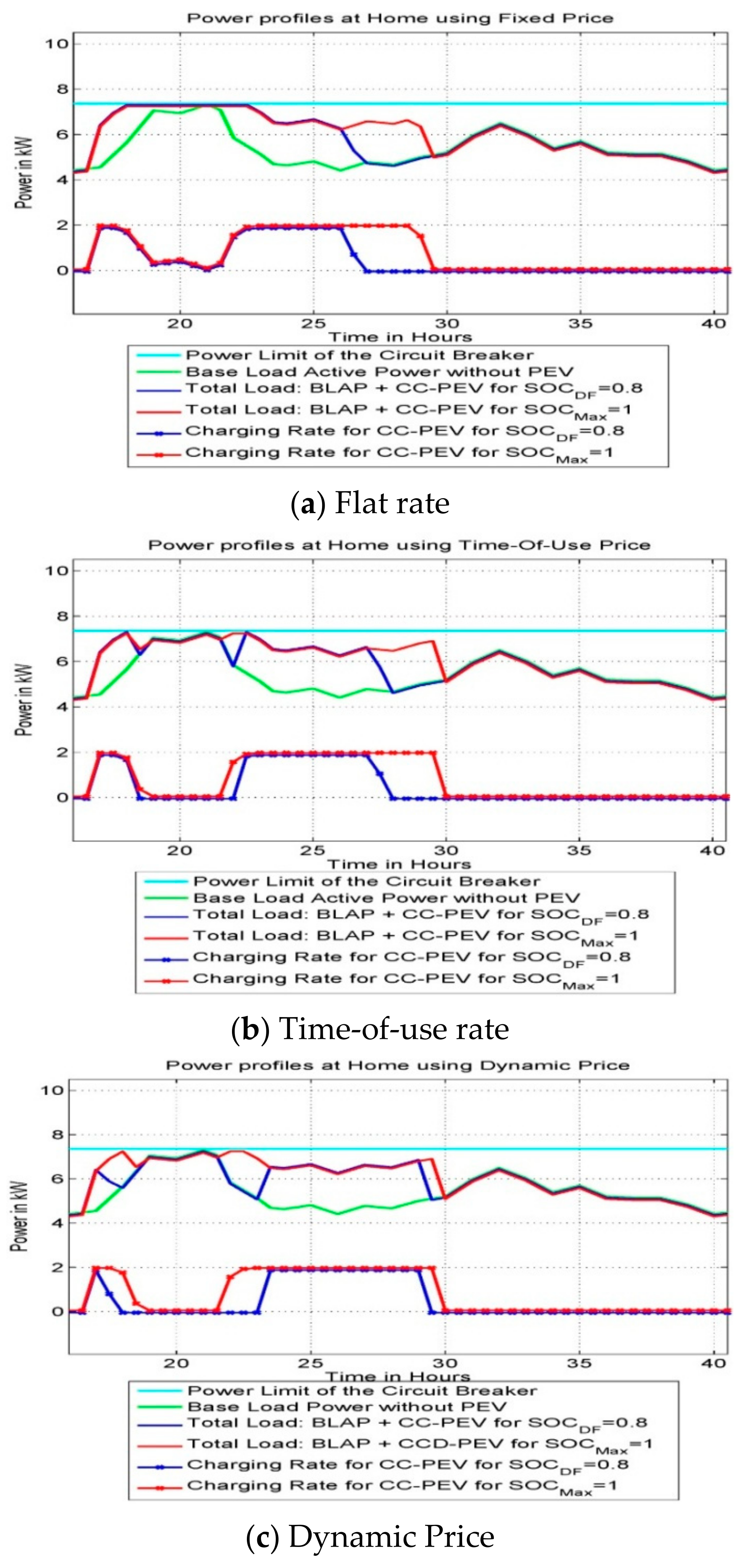
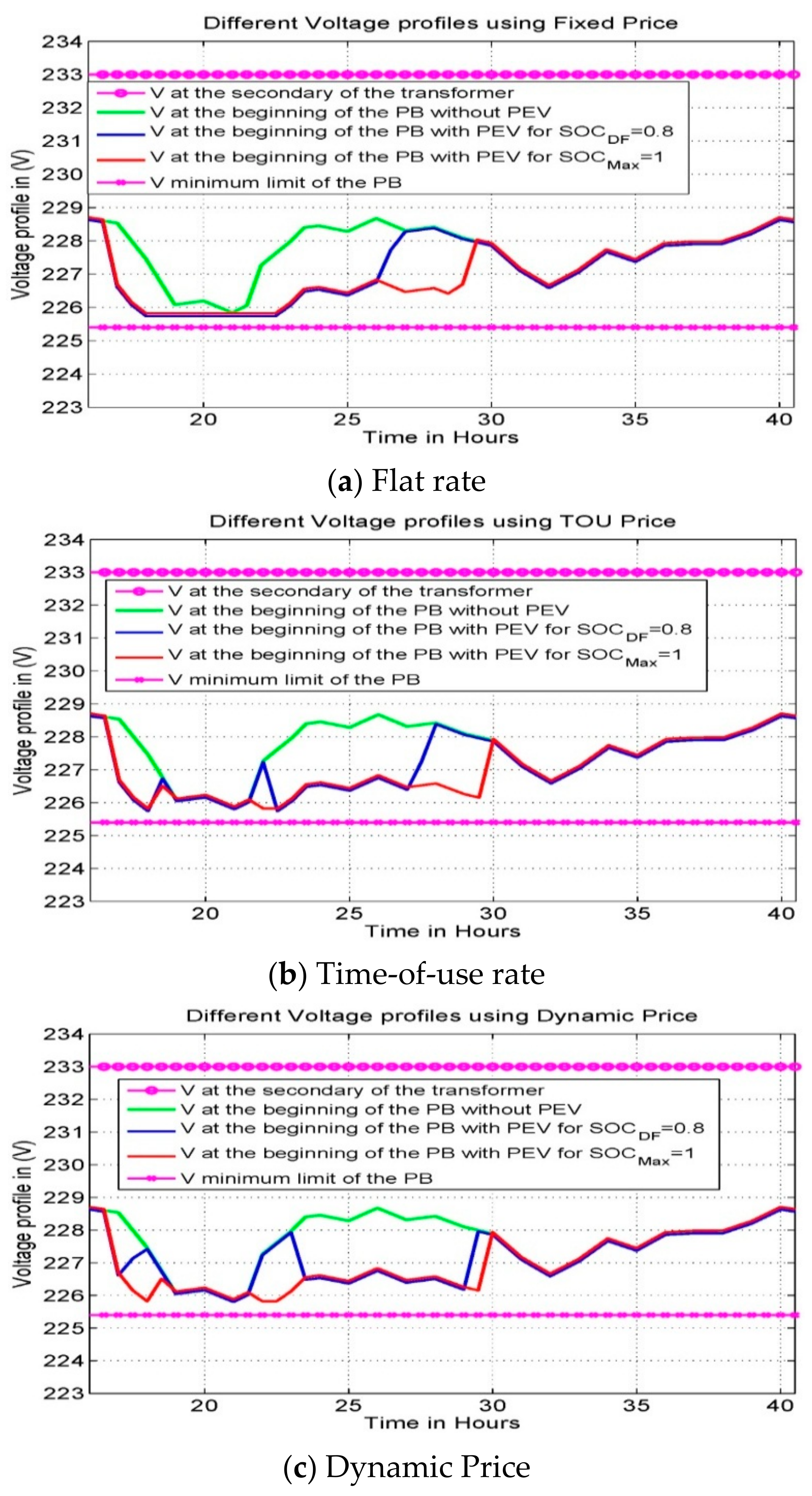
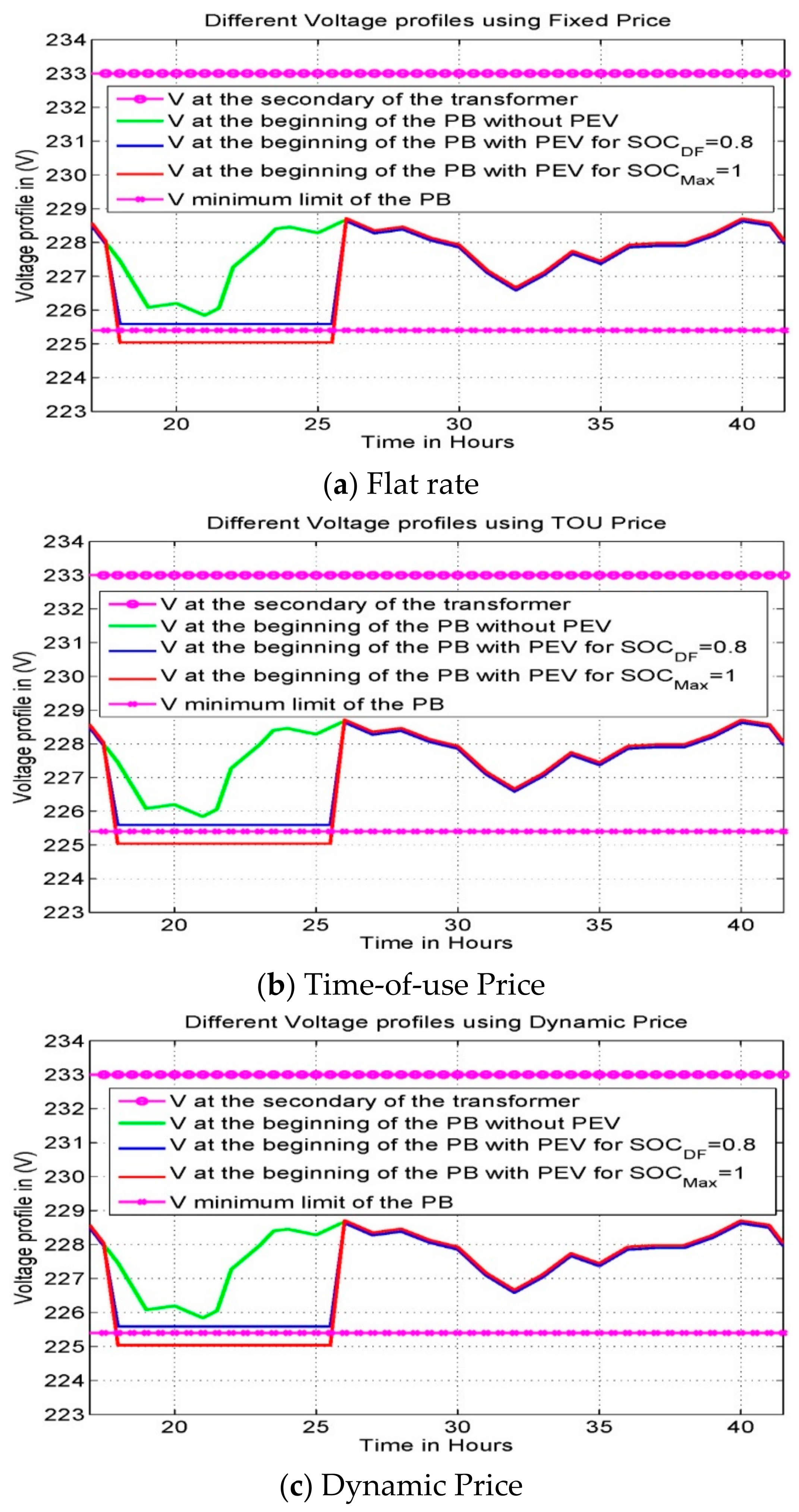
Figure 4 and Figure 5 show the profiles of the power and voltage at the home level for three cases, the baseload (BLAP), the total load with PEV and SOC D = 0.8 , and the total load with PEV and SOC D = 1 . At this point, everything seems well since the available energy at home is enough to charge the PEV. It can be remarked that the baseload power (power at home without PEV) is considered within the respected limit; the charging of PEV for SOC Max = 1 and SOC D = 0.8 respects the power limit imposed by the circuit breaker. For the TOU and dynamic pricing mechanisms, and for SOC Max = 1 , the PEV is obliged to charge during high price to reach the desired SOC level which will increase the cost of charging, while for SOC D = 0.8 the PEV is not charging during high prices, which will relax the charging mode and allow the algorithm to charge the PEV during low energy prices. The remaining SOC (1 − 0.8 = 0.2) will be charged later when the energy price is low.
Table 1, Table 2 and Table 3 represent the power quality under three different pricing mechanisms. It can be seen that the power losses and voltage drops are the least for the dynamic price compared to the TOU and fixed cost. Hence, results show how it is important to shift from the fixed cost to more sophisticated pricing mechanisms such as dynamic pricing. It can also be seen that charging the PEV to 80% instead of 100% reduced the power losses by 6.6%.
Table 4 presents the energy demand cost at home considering three distinct pricing mechanisms, (i) flat rate, (ii) time-of-use, and (iii) dynamic price. The second column shows the minimum, maximum, and total energy cost at home without PEV for each pricing mechanism. The third column represents the values of the home with PEV using coordinated charging, and the desired final SOC is SOC D = 0.8 . The remaining SOC (0.2) is charged later. The fourth column shows the results for the home with PEV using coordinated charging, and the final SOC is SOC Max = 1 . From Table 4, it is seen that when time-of-use and dynamic price are applied, and for the SOC D = 0.8 , the total energy cost is improved by 0.23% and 0.61%, respectively. If the owner charges his PEV every day, the gain per year for the time-of-use price is $0.0213 × 365 = $7.77, and for the dynamic price it is $0.06 × 365 = $21.9. The improvement is small because, in both cases, the optimization technique is used to find the best solution.

3.3. Case 2: Charging Time Is Insufficient to Charge the PEV within the Initial Constraints

In this subsection, the charging time is reduced and it is not sufficient for the PEV to fully charge its battery at the same power rate. Therefore, the PEV needs a higher power rate to charge its battery, and the recommended limit of the power may not be respected. The algorithm is modeled in a way to charge the PEV to the desired SOC level with the least power rate. Two different final SOCs are studied. The first one is when the PEV is charged to a SOC Max = 1 , and the second one is when the PEV is charged to a SOC D = 0.8 for the same period of time, but the rest of the energy (1 − 0.8 = 0.2) is charged later.
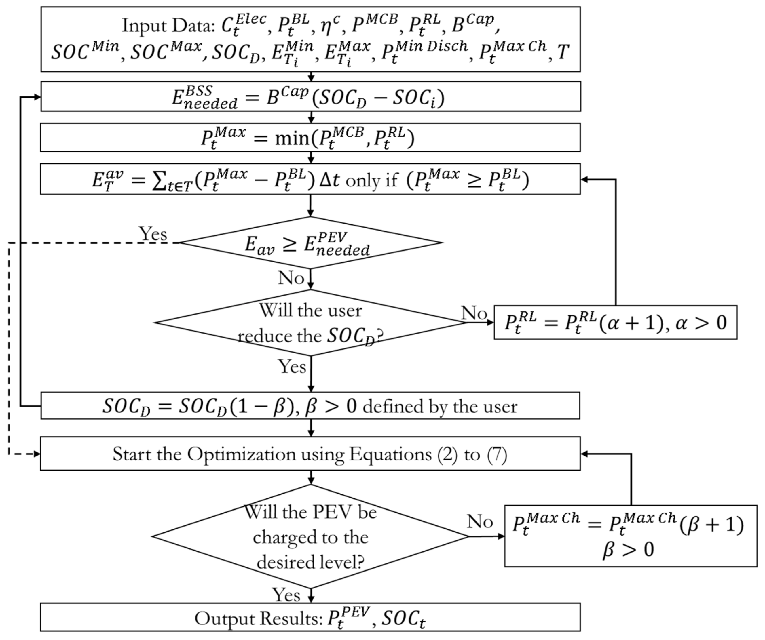
In this part, our proposed algorithm plays an important role in reducing the impact on the network and at-home levels. To calculate the available energy at home or transformer level, Equation (10) is used, which is more detailed than the one presented in the algorithm. The equation considers only the values of P t RL P t BL 0 , if a value of P t RL P t BL < 0 it will not be counted in the summation. This equation is valid for both SOC Max and SOC D .
t = t A t D Δ t 1 U P t BL P t RL · P t RL P t BL · Δ t SOC D SOC i · B Cap / η c
The left side of the equation represents the available energy on the bus, transformer, or at home to charge the PEV, while the right side represents the needed energy to charge the battery to the desired SOC level. If the equation on the left side is greater or equal to the equation on the right side, it means that there is sufficient energy to charge the battery. If the battery is not charged to the desired SOC level, it means that the charging power rate should be increased. However, if the equation on the left side is smaller than the equation on the right side, it means that there is no sufficient energy to charge the battery to the desired SOC level. To solve the problem, the P t RL should be increased in a way that the total available energy should be greater or equal to the needed energy to charge the battery. If the P t RL is increased and the battery is not charged to the desired SOC level, the charging power level should be increased. Hence, our proposed algorithm can solve all these problems.
In this subsection, the charging time is considered very small in that the PEV cannot charge its battery with the same power rate. Therefore, a higher power rate is recommended to attain the desired SOC level. Two different final SOCs are studied; the first one is when the PEV is charged to a SOC Max = 1 , and the second one is when the PEV is charged to a SOC D = 0.8 for the same period of time, but the rest of the energy (1 − 0.8 = 0.2) is charged later. Figure 6 represents the curves of two different SOCs. The first one is for SOC Max = 1 , and second one is for SOC D = 0.8 . It is clear that all curves for different pricing mechanisms have the same form due to the reduced period for charging. The algorithm is obliged to charge with the maximum power in order to attain the desired SOC level for difference pricing mechanisms.
In Figure 7, the baseload (load at home without PEV) is considered within the respected limit; the charging of PEV for SOC Max = 1 and SOC D = 0.8 could overpass the recommended limit because the PEV owner needs to charge his PEV to the desired SOC level, but the period for charging is small and not enough to charge the battery to the desired level with the current charging rate. Therefore, the P t RL is increased within the period of charging, and some power rates are also increased, as mentioned before. Hence, the PEV is charging at a high price, which will increase the electricity bill. For SOC D = 0.8 , the remaining SOC (1 − 0.8 = 0.2) will be charged later when the energy price is low.
In Figure 8, the voltage profile of the baseload respects the voltage limit imposed by the standard because the cable size is chosen to maintain the voltage drop within the respected limits when the power is less or equal to the circuit breaker nominal rate. The voltage profiles for the total load for SOC Max = 1 and SOC D = 0.8 may not respect the voltage limits imposed by the standards. This is due to the power, which has increased and overpassed the recommended limit in order to charge the battery to the desired SOC level during a short period of time. If the voltage drop is less but close to the recommended limit, it may not cause problems to home appliances, but a high voltage drop may cause problems at home, such as improper operation, and may damage some equipment and cause loss of energy and heating in some equipment. It can be seen that by reducing the SOC the voltage is maintained within the recommended limit, which emphasizes the importance of reducing the SOC.
Table 5, Table 6 and Table 7 present the power quality and losses at home. The first column represents the values of the home without PEV. The second column represents the values of the home with PEV when the desired final SOC is SOC D = 0.8 . The third column represents the values of the home with PEV, when the final SOC is SOC Max = 1 . It can be observed that charging the PEV to 80% instead of 100% reduces the power losses by 9% and the voltage drop by 14.5%, which is considered a good improvement.
Table 8 presents the energy demand cost at home considering three distinct pricing mechanisms, (i) flat rate, (ii) time-of-use, (iii) and dynamic price. The second column shows the minimum, maximum, and total energy cost at home without PEV for each pricing mechanism. The third column represents the values of the home with PEV, for SOC D = 0.8 . The remaining SOC (0.2) is charged later. The total cost is calculated. The fourth column shows the results of the home with PEV using coordinated charging, and the final SOC is SOC Max = 1 . From Table 8, it can be seen that when time-of-use and dynamic price are applied, and for SOC D = 0.8 , the total energy cost is improved by 0.916% and 0.81%, respectively. If the owner charges his PEV every day, the gained cost per year for the time-of-use price is ($10.515 − $10.4187) × 365 = $35.15, and for the dynamic price it is ($11.132 − $11.042) × 365 = $32.85. The improvement is not negligible. When the PEV needs a higher charging power rate to attain the desired SOC level, and for the TOU and dynamic prices, the PEV owner reduces the cost of charging if he charges his PEV to a SOC < 1, then the remaining energy is charged later when the energy price is low.
In this section, for the mentioned example, both studies do not respect the P t RL imposed by the circuit breaker of the home. The impact of the SOC D = 0.8 on the power profile is less than the SOC Max = 1 , where both studies overpass the required limit, but for SOC D = 0.8 , the limit is overpassed by a very small value. In both cases, the circuit breaker is tripped, but the case will be different for a bus, in which the transformer may not trip for SOC D = 0.8 , but it may trip for SOC Max = 1 because the limit is overpassed by a large value. For the voltage profile, the SOC D = 0.8 may not pass the limit imposed by the standards, while for the SOC Max = 1 , the limit may pass the standards. For the case of a transformer, overloading could increase the temperature of the transformer, thus decreasing its lifetime. Therefore, it is recommended to respect the limits imposed by the transformer’s limits and find other factors that will help the PEV to charge the battery to the desired SOC level without negatively affecting the circuit breaker and the transformer or other components on the network and home.

4. Conclusions

This paper investigated the impact of charging a Plug-in Electric Vehicle (PEV) at home under different State of Charge (SOC) levels and extreme conditions. An optimization algorithm was proposed that optimally schedules the charging process of a PEV and improves the convergence of the optimal solution even if the constraints are violated under extreme conditions, which was not done in other papers to the best of our knowledge. In addition, this paper has demonstrated that fully charging the PEV may create problems, especially during peak hours when a user urgently needs to charge his PEV. For this reason, it is suggested to charge the PEV to the desired SOC level that is less than the maximum capacity of the battery in certain unfavorable conditions, which meets the expectation of the car owner and at the same time reduces the impact on the network. The remaining energy can be charged later when the driver arrives at the destination point or while on his way. Results show that charging the PEV to a lower SOC level reduces the power losses and the voltage drop in some conditions, which is beneficial for the system operator. It can be concluded that it is not always beneficial to fully charge the PEV, especially when there are some peak demands, even if it is required by the car owner. Moreover, a SOC = 80% is often enough for the driver to arrive at his destination. The behavior of the car owner is very important even if an energy management system is used to optimally schedule the charging of the PEV.
This paper studied the impact at the home level; however, an investigation on the distribution network level is necessary to understand the behavior of car owners and the impact of charging the PEVs at different SOC levels, which will be done in our future work.

Author Contributions

Software, C.Z.E.-B.; validation, B.B., M.Z. and W.A.; formal analysis, C.Z.E.-B.; resources, U.E.; writing—original draft preparation, C.Z.E.-B.; writing—review and editing, B.B., M.Z., W.A. and U.E.; supervision, U.E.; funding acquisition, U.E. All authors have read and agreed to the published version of the manuscript.

Funding

This research was undertaken, in part, thanks to funding from the Canada Excellence Research Chairs Program. The funding source is the Tri-Agency Institutional Program Secretariat.

Conflicts of Interest

The authors declare no conflict of interest.

Nomenclature

BSSBattery storage system
DSODistribution System Operator
EVElectric Vehicle
MILPMixed Integer Linear Programming
PEVPlug-in Electric Vehicle
SOCState of Charge
TOUTime-of-Use price
B Cap Battery capacity (e.g., 100   kWh ).
C t Elec Electricity price at instant t during the period T
Δ t Time step (e.g., 0.5 h)
η c Charging efficiency of the battery (e.g., 0.95%)
E av Available energy at home in period T which is not used
E T i Min Minimum energy limit at home for the period T i T
E T i Max Maximum energy limit at home for the period T i T
E needed PEV Needed energy to charge the battery to the desired State of Charge level
P t Max Maximum power limit
P t Max   Ch Maximum charging limit at instant “t” of the Plug-in Electric Vehicle
P t Min   Disch Minimum discharging limit at instant “t” of the Plug-in Electric Vehicle
P MCB Main circuit breaker power rating (e.g., 6.4 kW)
P t PEV Power demand of the Plug-in Electric Vehicle
P t BL Baseload power profile at home
P t Max Maximum power limit at home that should not be exceeded
SOC D Desired Final State of Charge
SOC f Final State of Charge
SOC i Initial State of Charge
SOC Min Minimum State of Charge of the battery
SOC Max Maximum State of Charge of the battery
T Period of the study (e.g., 24 h)

References

  1. Ajanovic, A. The future of electric vehicles: Prospects and impediments. Wiley Interdiscip. Rev. Energy Environ. 2015, 4, 521–536. [Google Scholar] [CrossRef]
  2. Sperling, D. Future Drive: Electric Vehicles and Sustainable Transportation; Island Press: Washington, DC, USA, 2013. [Google Scholar]
  3. Huda, M.; Aziz, M.; Tokimatsu, K. The future of electric vehicles to grid integration in Indonesia. Energy Procedia 2019, 158, 4592–4597. [Google Scholar] [CrossRef]
  4. Gustafsson, T.; Johansson, A. Comparison between Battery Electric Vehicles and Internal Combustion Engine Vehicles Fueled by Electrofuels-From an Energy Efficiency and Cost Perspective. Master’s Thesis, Department of Energy and Environment, Chalmers University of Technology, Gothenburg, Sweden, 2015. [Google Scholar]
  5. Satarworn, S.; Hoonchareon, N. Impact of EV home charger on distribution transformer overloading in an urban area. In Proceedings of the 2017 14th International Conference on Electrical Engineering/Electronics Computer, Telecommunications and Information Technology (ECTI-CON), Phuket, Thailand, 27–30 June 2017; pp. 469–472. [Google Scholar]
  6. Marcincin, O.; Medvec, Z.; Moldrik, P. The impact of electric vehicles on distribution network. In Proceedings of the 2017 18th International Scientific Conference on Electric Power Engineering (EPE), Kouty nad Desnou, Czech Republic, 17–19 May 2017; pp. 1–5. [Google Scholar]
  7. Ramaswamy, P.C.; Chardonnet, C.; Rapoport, S.; Czajkowski, C.; Sanchez, R.R.; Arriola, I.G.; Bulto, G.O. Impact of electric vehicles on distribution network operation: Real world case studies. In Proceedings of the CIRED Workshop 2016, Helsinki, Finland, 14–15 June 2016; pp. 1–5. [Google Scholar]
  8. Tan, K.M.; Ramachandaramurthy, V.K.; Yong, J.Y. Integration of electric vehicles in smart grid: A review on vehicle to grid technologies and optimization techniques. Renew. Sustain. Energy Rev. 2016, 53, 720–732. [Google Scholar] [CrossRef]
  9. Yong, J.Y.; Ramachandaramurthy, V.K.; Tan, K.M.; Mithulananthan, N. A review on the state-of-the-art technologies of electric vehicle, its impacts and prospects. Renew. Sustain. Energy Rev. 2015, 49, 365–385. [Google Scholar] [CrossRef]
  10. Habib, S.; Kamran, M.; Rashid, U. Impact analysis of vehicle-to-grid technology and charging strategies of electric vehicles on distribution networks—A review. J. Power Sources 2015, 277, 205–214. [Google Scholar] [CrossRef]
  11. El-Bayeh, C.Z.; Eicker, U.; Alzaareer, K.; Brahmi, B.; Zellagui, M. A Novel Data-Energy Management Algorithm for Smart Transformers to Optimize the Total Load Demand in Smart Homes. Energies 2020, 13, 4984. [Google Scholar] [CrossRef]
  12. El-Bayeh, C.Z.; Alzaareer, K.; Brahmi, B.; Zellagui, M. A Novel Algorithm for Controlling Active and Reactive Power Flows of Electric Vehicles in Buildings and Its Impact on the Distribution Network. World Electr. Veh. J. 2020, 11, 43. [Google Scholar] [CrossRef]
  13. El-Bayeh, C.Z.; Mougharbel, I.; Saad, M.; Chandra, A.; Asber, D.; Lenoir, L.; Lefebvre, S. Novel Soft-Constrained Distributed Strategy to meet high penetration trend of PEVs at homes. Energy Build. 2018, 178, 331–346. [Google Scholar] [CrossRef]
  14. Zhang, L.; Li, Y. A Game-Theoretic Approach to Optimal Scheduling of Parking-Lot Electric Vehicle Charging. IEEE Trans. Veh. Technol. 2016, 65, 4068–4078. [Google Scholar] [CrossRef]
  15. Mohsenzadeh, A.; Pazouki, S.M.; Haghifam, R.; Chengzong, P. Optimal planning of parking lots and demand response programs in distribution network considering power loss and voltage profile. In Proceedings of the 2015 IEEE Power & Energy Society Innovative Smart Grid Technologies Conference (ISGT), Washington, DC, USA, 18–20 February 2015; pp. 1–5. [Google Scholar]
  16. Yong, J.Y.; Ramachandaramurthy, V.K.; Tan, K.M.; Mithulananthan, N. Bi-directional electric vehicle fast charging station with novel reactive power compensation for voltage regulation. Int. J. Electr. Power Energy Syst. 2015, 64, 300–310. [Google Scholar] [CrossRef]
  17. Anand, D.M.; de Salis, R.T.; Cheng, Y.; Moyne, J.; Tilbury, D.M. A Hierarchical Incentive Arbitration Scheme for Coordinated PEV Charging Stations. IEEE Trans. Smart Grid 2015, 6, 1775–1784. [Google Scholar] [CrossRef]
  18. El-Bayeh, C.Z.; Mougharbel, I.; Saad, M.; Chandra, A.; Lefebvre, S.; Asber, D.; Lenoir, L. A detailed review on the parameters to be considered for an accurate estimation on the Plug-in Electric Vehicle’s final State of Charge. In Proceedings of the 2016 3rd International Conference on Renewable Energies for Developing Countries (REDEC), Zouk Mosbeh, Lebanon, 13–15 July 2016; pp. 1–6. [Google Scholar]
  19. El-Bayeh, C.Z.; Alzaareer, K.; Aldaoudeyeh, A.-M.I.; Brahmi, B.; Zellagui, M. Charging and Discharging Strategies of Electric Vehicles: A Survey. World Electr. Veh. J. 2021, 12, 11. [Google Scholar] [CrossRef]
  20. Melhem, F.Y.; Grunder, O.; Hammoudan, Z.; Moubayed, N. Energy Management in Electrical Smart Grid Environment Using Robust Optimization Algorithm. IEEE Trans. Ind. Appl. 2018, 54, 2714–2726. [Google Scholar] [CrossRef]
  21. Amjad, M.; Ahmad, A.; Rehmani, M.H.; Umer, T. A review of EVs charging: From the perspective of energy optimization, optimization approaches, and charging techniques. Trans. Res. Part D Trans. Environ. 2018, 62, 386–417. [Google Scholar] [CrossRef]
  22. El-Bayeh, C.Z.; Mougharbel, I.; Saad, M.; Chandra, A.; Asber, D.; Lefebvre, S. Impact of Considering Variable Battery Power Profile of Electric Vehicles on the Distribution Network. In Proceedings of the 2018 4th International Conference on Renewable Energies for Developing Countries (REDEC), Beirut, Lebanon, 1–2 November 2018; pp. 1–8. [Google Scholar]
  23. Alzaareer, K.; Saad, M.; Mehrjerdi, H.; El-Bayeh, C.Z.; Asber, D.; Lefebvre, S. A new sensitivity approach for preventive control selection in real-time voltage stability assessment. Int. J. Electr. Power Energy Syst. 2020, 122, 106212. [Google Scholar] [CrossRef]
  24. de Hoog, J.; Muenzel, V.; Jayasuriya, D.C.; Alpcan, T.; Brazil, M.; Thomas, D.; Mareels, I.; Dahlenburg, G.; Jegatheesan, R. The importance of spatial distribution when analysing the impact of electric vehicles on voltage stability in distribution networks. Energy Syst. 2015, 6, 63–84. [Google Scholar] [CrossRef]
  25. Zhang, C.; Chen, C.; Sun, J.; Zheng, P.; Lin, X.; Bo, Z. Impacts of electric vehicles on the transient voltage stability of distribution network and the study of improvement measures. In Proceedings of the 2014 IEEE PES Asia-Pacific Power and Energy Engineering Conference (APPEEC), Hong Kong, China, 7–10 December 2014; pp. 1–6. [Google Scholar]
  26. Hussain, S.; El-Bayeh, C.Z.; Lai, C.; Eicker, U. Multi-Level Energy Management Systems toward a Smarter Grid: A Review. IEEE Access 2021, 9, 71994–72016. [Google Scholar] [CrossRef]
  27. El-Bayeh, C.; Mougharbel, I.; Saad, M.; Chandra, A.; Lefebvre, S.; Asber, D. Novel multilevel soft constraints at homes for improving the integration of plug-in electric vehicles. In Proceedings of the 2018 4th International Conference on Renewable Energies for Developing Countries (REDEC), Beirut, Lebanon, 1–2 November 2018; pp. 1–9. [Google Scholar]
  28. Hoke, A.; Brissette, A.; Maksimović, D.; Pratt, A.; Smith, K. Electric vehicle charge optimization including effects of lithium-ion battery degradation. In Proceedings of the 2011 IEEE Vehicle Power and Propulsion Conference, Chicago, IL, USA, 6–9 September 2011; pp. 1–8. [Google Scholar]
  29. Arif, S.; Lie, T.; Seet, B.; Ayyadi, S.; Jensen, K. Review of Electric Vehicle Technologies, Charging Methods, Standards and Optimization Techniques. Electronics 2021, 10, 1910. [Google Scholar] [CrossRef]
  30. Ahn, C.; Li, C.-T.; Peng, H. Optimal decentralized charging control algorithm for electrified vehicles connected to smart grid. J. Power Sources 2011, 196, 10369–10379. [Google Scholar] [CrossRef]
  31. Sundstrom, O.; Binding, C. Flexible Charging Optimization for Electric Vehicles Considering Distribution Grid Constraints. IEEE Trans. Smart Grid 2012, 3, 26–37. [Google Scholar] [CrossRef]
  32. Khodayar, M.E.; Wu, L.; Shahidehpour, M. Hourly Coordination of Electric Vehicle Operation and Volatile Wind Power Generation in SCUC. IEEE Trans. Smart Grid 2012, 3, 1271–1279. [Google Scholar] [CrossRef]
  33. Yifeng, H.; Venkatesh, B.; Ling, G. Optimal Scheduling for Charging and Discharging of Electric Vehicles. IEEE Trans. Smart Grid 2012, 3, 1095–1105. [Google Scholar]
Figure 1. Proposed algorithm to schedule the charging of PEVs.
Energies 14 06589 g001
Figure 2. Three electricity rates are used, flat rate, time-of-use, and dynamic price.
Energies 14 06589 g002
Figure 3. SOC of the Battery for SOC Max = 1 and SOC D = 0.8 , for (a) Flat rate, (b) TOU, (c) Dynamic price.
Energies 14 06589 g003
Figure 4. Power profiles for SOC Max = 1 and SOC D = 0.8 , for (a) Flat rate, (b) TOU, (c) Dynamic price.
Energies 14 06589 g004
Figure 5. Voltage profiles for SOC Max = 1 and SOC D = 0.8 , for (a) Flat rate, (b) TOU, (c) Dynamic price.
Energies 14 06589 g005
Figure 6. SOC of the Battery for SOC Max = 1 and SOC D = 0.8 , for (a) Flate rate, (b) TOU, (c) Dynamic price.
Energies 14 06589 g006
Figure 7. Power profiles for SOC Max = 1 and SOC D = 0.8 , for (a) Flate rate, (b) TOU, (c) Dynamic price.
Energies 14 06589 g007
Figure 8. Voltage profiles for the baseload and total load for SOC Max = 1 and SOC D = 0.8 , for (a) Flate rate, (b) TOU, (c) Dynamic price.
Energies 14 06589 g008
Table 1. Power demand and loss, current and voltage at home (flat rate).
ElementUnitWithout PEVsWith PEV and SOC D F   =   0.8 With PEV and SOC Max   =   1
Circuit BreakerkW7.36 kW7.36 kW7.36 kW
LoadkW4.4095 Min4.4186 Min4.4186 Min
7.3001 Max7.3600 Max7.3600 Max
Circuit BreakerA40 A40 A40 A
40 AA23.9645 Min24.0143 Min24.0143 Min
39.6747 Max40.0000 Max40.0000 Max
VoltageV225.84 Min225.78 Min225.78 Min
228.68 Max228.67 Max228.67 Max
Voltage Drop%0.5758 Min0.5798 Min0.5798 Min
1.8085 Max1.8340 Max1.8340 Max
Power LosseskW0.0648 Min0.0650 Min0.0650 Min
0.1775 Max0.1805 Max0.1805 Max
4.9058 Total5.9337 Total6.3283 Total
0.0000%+20.9547%+28.9984%
Table 2. Power demand and loss, current and voltage at home (time-of-use).
ElementUnitWithout PEVsWith PEV and S O C D F   =   0.8 With PEV and S O C M a x   =   1
Circuit BreakerkW7.36 kW7.36 kW7.36 kW
LoadkW4.4095 Min4.4186 Min4.4186 Min
7.3001 Max7.3600 Max7.3600 Max
Circuit BreakerA40 A40 A40 A
Line currentA23.9645 Min24.0143 Min24.0143 Min
39.6747 Max40.0000 Max40.0000 Max
VoltageV225.84 Min225.78 Min225.78 Min
228.68 Max228.67 Max228.67 Max
Voltage Drop%0.5758 Min0.5798 Min0.5798 Min
1.8085 Max1.8340 Max1.8340 Max
Power LosseskW0.0648 Min0.0650 Min0.0650 Min
0.1775 Max0.1805 Max0.1805 Max
4.9058 Total5.8993 Total6.3132 Total
0.0000%+20.2534%+28.6891%
Table 3. Power demand and loss, current and voltage at home (dynamic price).
ElementUnitWithout PEVsWith PEV and S O C D F   =   0.8 With PEV and S O C M a x   =   1
Circuit BreakerkW7.36 kW7.36 kW7.36 kW
LoadkW4.4095 Min4.4186 Min4.4186 Min
7.3001 Max7.3001 Max7.3600 Max
Circuit BreakerA40 A40 A40 A
Line currentA23.9645 Min24.0143 Min24.0143 Min
39.6747 Max39.6747 Max40.0000 Max
VoltageV225.84 Min225.84 Min225.84 Min
228.68 Max228.67 Max228.67 Max
Voltage Drop%0.5758 Min0.5798 Min0.5798 Min
1.8085 Max1.8085 Max1.8085 Max
Power LosseskW0.0648 Min0.0650 Min0.0650 Min
0.1775 Max0.1775 Max0.1805 Max
4.9058 Total5.8770 Total6.3132 Total
0.0000%+19.7978%+28.6891%
Table 4. Energy cost at home.
Pricing MechanismWithout PEVWith PEV and S O C D F   =   0.8
+0.2 Charged Later
With PEV and S O C M a x   =   1
Flat rate ($)0.15146 Min0.15146 Min0.15146 Min
0.25076 Max0.25282 Max0.25282 Max
8.9678 Total10.2090 Total10.2090 Total
Time-Of-Use ($)0.13228 Min0.13228 Min0.13228 Min
0.36501 Max0.36501 Max0.36501 Max
9.2427 Total10.3267 Total10.3480 Total
Dynamic Price ($)0.13132 Min0.13132 Min0.13132 Min
0.35992 Max0.35992 Max0.35992 Max
9.8060 Total10.9440 Total11.004 Total
Table 5. Power demand and loss, current and voltage at home (flat rate).
ElementUnitWithout PEVsWith PEV and S O C D F   =   0.8 With PEV and S O C M a x   =   1
Circuit BreakerkW7.36 kW7.36 kW7.36 kW
LoadkW4.4095 Min4.4095 Min4.4095 Min
7.3001 Max7.5134 Max8.1586 Max
Circuit BreakerA40 A40 A40 A
Line currentA23.9645 Min23.9645 Min23.9645 Min
39.6747 Max40.8338 Max44.3401 Max
VoltageV225.84 Min225.63 Min225.00 Min
228.68 Max228.68 Max228.68 Max
Voltage Drop%0.5758 Min0.5758 Min0.5759 Min
1.8085 Max1.8994 Max2.1745 Max
Power LosseskW0.0648 Min0.0648 Min0.0649 Min
0.1775 Max0.1881 Max0.2217 Max
4.9431 Total6.0403 Total6.5792 Total
0.0000%+22.1962%+33.0987%
Table 6. Power demand and loss, current and voltage at home (time-of-use).
ElementUnitWithout PEVsWith PEV and S O C D F   =   0.8 With PEV and S O C M a x   =   1
Circuit BreakerkW7.36 kW7.36 kW7.36 kW
LoadkW4.4095 Min4.4095 Min4.4095 Min
7.3001 Max7.5134 Max8.1586 Max
Circuit BreakerA40 A40 A40 A
Line currentA23.9645 Min23.9645 Min23.9645 Min
39.6747 Max40.8338 Max44.3401 Max
VoltageV225.84 Min225.63 Min225.00 Min
228.68 Max228.68 Max228.68 Max
Voltage Drop%0.5758 Min0.5758 Min0.5759 Min
1.8085 Max1.8994 Max2.1745 Max
Power LosseskW0.0648 Min0.0648 Min0.0648 Min
0.1775 Max0.1881 Max0.2217 Max
4.9431 Total6.0403 Total6.5792 Total
0.0000%+22.1962%+33.0987%
Table 7. Power demand and loss, current and voltage at home (dynamic price).
ElementUnitWithout PEVsWith PEV and S O C D F   =   0.8 With PEV and S O C M a x   =   1
Circuit BreakerkW7.36 kW7.36 kW7.36 kW
LoadkW4.4095 Min4.4095 Min4.4095 Min
7.3001 Max7.5134 Max8.1586 Max
Circuit BreakerA40 A40 A40 A
Line currentA23.9645 Min23.9645 Min23.9645 Min
39.6747 Max40.8338 Max44.3401 Max
VoltageV225.84 Min225.63 Min225.63 Min
228.68 Max228.68 Max228.68 Max
Voltage Drop%0.5758 Min0.5758 Min0.5759 Min
1.8085 Max1.8994 Max2.1745 Max
Power LosseskW0.0648 Min0.0648 Min0.0648 Min
0.1775 Max0.1881 Max0.2217 Max
4.9431 Total6.0403 Total6.5792 Total
0.0000%+22.1962%+33.0987%
Table 8. Energy Cost at Home Per Day ($/Day).
Pricing MechanismWithout PEVWith PEV and S O C D F   =   0.8
+0.2 Charged Later
With PEV and S O C M a x   =   1
Flat Rate ($)0.15146 Min0.15146 Min0.15146 Min
0.25076 Max0.25809 Max0.28025 Max
8.9678 Total10.2090 Total10.2090 Total
Time-Of-Use ($)0.13228 Min0.13228 Min0.13228 Min
0.36501 Max0.37567 Max0.40793 Max
9.2427 Total10.4187 Total10.5150 Total
Dynamic Price ($)0.13132 Min0.13132 Min0.13132 Min
0.35992 Max0.37044 Max0.40225 Max
9.8060 Total11.0420 Total11.1320 Total
Publisher’s Note: MDPI stays neutral with regard to jurisdictional claims in published maps and institutional affiliations.

