Learning Feedforward Control Using Multiagent Control Approach for Motion Control Systems

Abstract

Multiagent control system (MACS) has become a promising solution for solving complex control problems. Using the advantages of MACS-based design approaches, a novel solution for advanced control of mechatronic systems has been developed in this paper. The study has aimed at integrating learning control into MACS. Specifically, learning feedforward control (LFFC) is implemented as a pattern for incorporation in MACS. The major novelty of this work is that the feedback control part is realized in a real-time periodic MACS, while the LFFC algorithm is done on-line, asynchronously, and in a separate non-real-time aperiodic MACS. As a result, a MACS-based LFFC design method has been developed. A second-order B-spline neural network (BSN) is used as a function approximator for LFFC whose input-output mapping can be adapted during control and is intended to become equal to the inverse model of the plant. To provide real-time features for the MACS-based LFFC system, the open robot control software (OROCOS) has been employed as development and runtime environment. A case study using a simulated linear motor in the presence of nonlinear cogging and friction force as well as mass variations is used to illustrate the proposed method. A MACS-based LFFC system has been designed and implemented for the simulated plant. The system consists of a setpoint generator, a feedback controller, and a time-index LFFC that can learn on-line. Simulation results have demonstrated the applicability of the design method.

1. Introduction

When designing control systems for mechatronic systems (in particular, precise motion control applications using electric motors), in order to achieve both high performance and robustness, one needs to take into account three issues: (1) reduction of the influence of plant disturbances, (2) attenuation of the undesired effect of measurement noise, and (3) handling of model uncertainties. By applying classical model-based feedback controllers, such as proportional integral derivative (PID) or linear quadratic Gaussian (LQG), designers have to face two difficulties [1]: (i) the design of a feedback controller often requires extensive effort and time consuming in modelling to obtain a good model of the process or plant; (ii) a compromise has to be made between performance and robust stability. The latter means that it is difficult to obtain simultaneously high-performance and robust stability in the presence of model uncertainties, plant disturbances, and measurement noise. This is indeed the place where learning and adaptive controllers may be considered, for example: adaptive control [2,3,4], iterative learning control [5,6], and learning feedforward control [1,7,8,9,10,11,12,13,14,15,16].

Learning feedforward control (LFFC), as shown in Figure 1, was originally proposed for electromechanical systems to compensate reproducible disturbances such that high-performance robust motion control systems can be achieved [1,10]. The input of the LFFC can be either the reference position and its derivatives (e.g., velocity, acceleration) or the periodic motion time in case of repetitive motions. As a two degrees of freedom (2-DoF) control structure, LFFC generates feedforward control signals that enhance the feedback control performance and make the output of the process follow the reference signal. As a result, feedback and feedforward part contributes independently control signals to overcoming the effect of disturbances as well as handling the uncertainties in plant model. The use of LFFC can improve not only the disturbance rejection, but also the stability robustness of the controlled system [9]. In essence, the learning feedforward controller in this scheme is designed as a function approximator that tries to imitate the inverse model of the plant [8,12]. Basically, LFFC is similar to performing system identification, however instead of learning based on the output of the system, it learns by minimizing the error of the feedback control signal. Instead of using the error directly, the output of the feedback controller is chosen as a training signal for the LFFC. This choice is based on the intuitive reasoning that this signal is the feedback controller’s best guess on how to decrease the tracking error [9]. Due to its simplicity and effectiveness, LFFC has been widely applied in many areas, such as robotics [11], linear motors [8,10,13], piezoelectric actuators [14], uninterruptible power supply (UPS) inverters [15], and refrigeration systems [16]. Two different types of neural networks are often used as function approximators, that is, multilayer perceptron (MLP) network and B-spline neural networks (BSN) [1,11,14,15,16].

It is assumed that in an adaptive or learning control scheme like LFFC, the learning activity always requires a long computation time (mostly in seconds) so that it should not be implemented in the same real-time periodic task, which is employed for feedback control with sampling time typically required in milliseconds. Hence, the work presented in this paper has searched for a new solution for the research problem: How to design and implement LFFC in a way that the feedback control activity is realized in a real-time periodic task, while the learning feedforward control algorithm can be done on-line, asynchronously, and in a separate non-real-time aperiodic task?

Scheduling periodic and aperiodic tasks in (hard) real-time computing systems has been intensively investigated in the literature, such as by the work in [17,18,19,20,21]. In a simple description, a periodic task is one which repeats itself after a fixed time interval, whereas an aperiodic task can arrive for execution at any time [18]. In other words, tasks that require regular activations are called periodic, whereas tasks which have irregular arrival times are called aperiodic [19].

The multicontroller approach [22,23] is well known to be a potential solution for the research problem, where a complex or advanced control system can be divided into several simple control tasks (or components). Then the most challenging problem of this approach is the design of a supervisory system (or a supervisor) to integrate many mixed real-time periodic and non-real-time aperiodic tasks and to deal with the integration and scheduling aspects of these components in a central way. In this case, scheduling real-time periodic tasks (feedback control part) and non-real-time aperiodic tasks (learning feedforward control part) to meet their time constraints is an important issue in the design of LFFC using a supervisor-based multicontroller approach. The task scheduling algorithm must satisfy the deadlines of real-time periodic tasks and provide fast response times for non-real-time aperiodic tasks. The development of this algorithm requires high embedded system development skills as well as real-time computing knowledge. Moreover, one has to design and implement a supervisory system for each particular control system (LFFC in this case). If the control system structure is modified then the supervisory system must be redesigned and reimplemented. For example, when the composition of real-time periodic and non-real-time aperiodic tasks is changed then the supervisory system must be designed again from the beginning. As a result, the supervisor-based multicontroller approach would usually lead to an overcomplicated supervisory system.

Over the last two decades, multiagent system (MAS) technology has been suggested as a promising solution for solving complex control problems in manufacturing and mechatronic systems, as discussed in [24,25,26,27,28,29,30,31,32], because of its ability to provide many advantages such as reusability, robustness, flexibility, adaptability, and scalability. In the research [33], the concept of agent from the field of MAS has been merged with the concept of controller of the control engineering discipline to form the concept of controller-agent. This combination results in the so-called multiagent control system (MACS) with hierarchical structure. Following the work in [33], this study has proposed a novel solution using the MACS-based design approach for LFFC. The research aims at combining the advantages of adaptive/learning control and agent-based control to form a new multiagent-based LFFC method. To the best of our knowledge, the proposal of integrating LFFC into MACS has not been previously reported in the literature. Also, in order to provide real-time features for multiagent-based LFFC systems, the Open Robot Control Software (OROCOS) framework [34] is used as the real-time control platform. It should be mentioned that the work in [35] tried to implement this approach. However, the attempt was only able to implementing LFFC using OROCOS, i.e., it was not successful in deploying LFFC within the MACS context.

In summary, a novel solution for advanced control of mechatronic systems has been proposed in this study. The work aims at integrating learning control into MACS. Specifically, LFFC will be implemented as a pattern for incorporation in MACS. The major novelty of this work is that the feedback control part is realized in a real-time periodic MACS, while the learning feedforward control algorithm is done on-line, asynchronously, and in a separate non-real-time aperiodic MACS. As a result, a MACS-based LFFC design method has been developed by the work presented in this paper.

The remaining of the paper is structured as follows. Section 2 briefly introduces OROCOS framework and hierarchically structured multiagent control system (MACS) using coordination mechanisms. Section 3 describes a case study using a simulated linear motor with nonlinear disturbances and presents the design of a MACS-based time-index LFFC system for the linear motor. Section 4 presents the simulation results. Finally, the paper is concluded and discussed in Section 5.

2. Background and Related Works

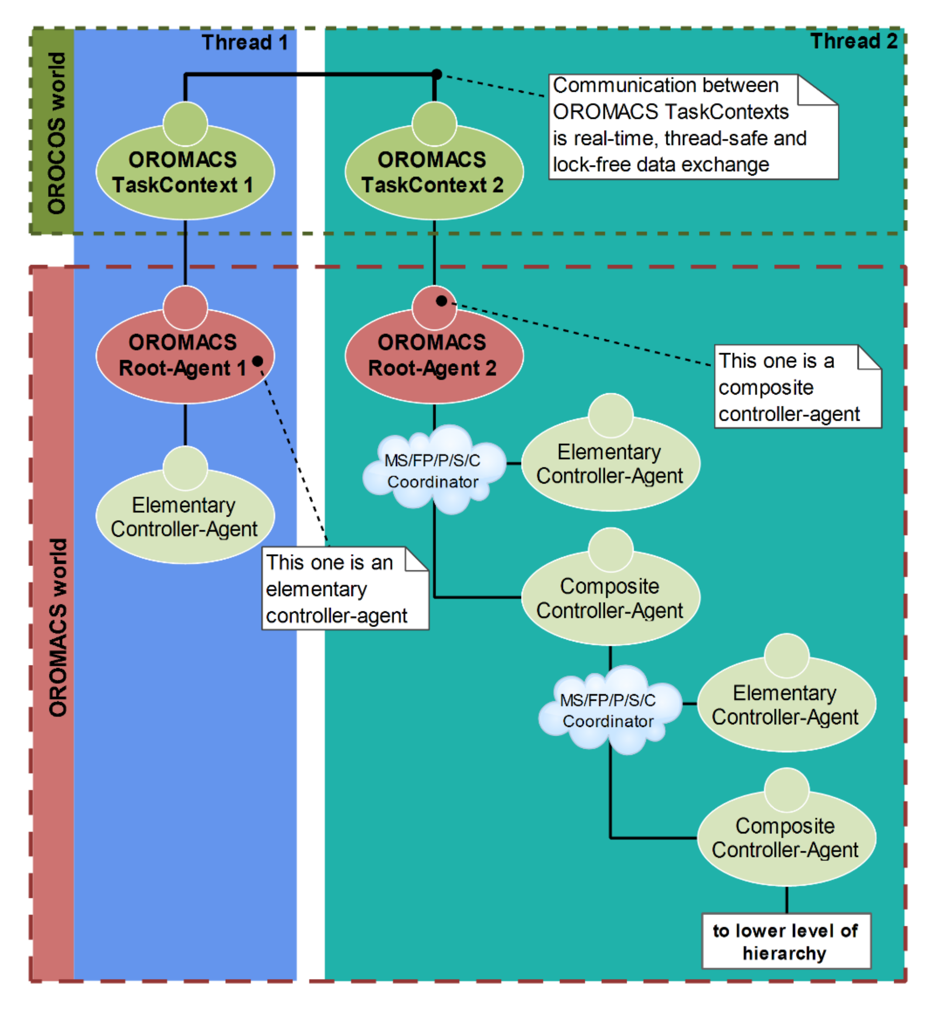
2.1. OROCOS Framework

Open Robot Control Software (OROCOS) is a software framework for general robot/machine control that provides a real-time toolkit to develop component-based real-time control applications [34,36]. In the OROCOS framework, a component is a basic unit of functionality that executes one or more (real-time) programs or tasks in a single thread. However, multithreaded components can be built such that they form real-time, thread-safe robot/machine control applications [37,38]. Components in OROCOS are implemented by subclassing the C++ TaskContext class. So, an OROCOS component is also called a TaskContext. In a simple description, TaskContext defines the “context” in which application-specific tasks are executed. A TaskContext is described through five primitives, i.e., attributes and properties, commands, methods, events, and data flow ports [38]. The interface between TaskContexts is implemented based on these primitives. When a TaskContext is running, it accepts commands and events using its execution engine. The execution engine will check periodically for new commands in its queue and execute programs which are running in the task. Data flow goes through ports and is manipulated by algorithms in the TaskContext [38].

In OROCOS, each TaskContext has ports in order to send or receive a stream of data. A user’s algorithm writes output ports to publish data to other TaskContexts, while input ports allow an algorithm to receive data from other TaskContexts. Reading and writing data ports is always (hard) real-time and thread-safe [38]. Furthermore, real-time components can communicate with non-real-time components (and vice versa) transparently. For a more detailed description of OROCOS, potential readers are referred to [34,38].

2.2. Multiagent Control System (MACS)

The work in [33] has developed a controller-agent-based design framework (named OROMACS) for the construction of hierarchically structured MACS for mechatronic systems. In OROMACS, the implementation of local controllers is based on the concept of agents, giving the so-called controller-agents; and multicontroller systems thus lead to the concept of the multiagent control system (MACS). In a MACS, multiple controller-agents act on their own particular problems to solve the overall problem so conflicts between individual controller-agents may arise. The conflicts are resolved by means of coordination mechanisms (or coordinators) between controller-agents. The coordinator determines when and how activities of controller-agents (e.g., calculation of control signals) are applied to the plant. There are five main types of coordination mechanisms (or coordinators), which are essential for the development of MACS [33]:

• Fixed-Priority (FP) coordinator: each controller-agent in a MACS is assigned a fixed priority index. Only one controller-agent in a MACS may be active at a particular time instance. The controller-agent with the highest priority level that wants to be active, gets active. If the highest priority controller-agent does not want to be active (or after it turns into inactive), the next controller-agent in the list of priority levels can be active and so on.
• Master–Slave (MS) coordinator makes controller-agents in a MACS operate in a way that the slave-controller-agent(s) can be active only after the master-controller-agent is active.
• Parallel (P) coordinator makes controller-agents in a MACS be active concurrently. In other words, all controller-agents in a MACS work independently. When a controller-agent wants to get active, it gets active, independent of the other controller-agents.
• Sequential (S) coordinator makes controller-agents in a MACS become active in succession (or a sequential order) for only one round. When a particular controller-agent gets inactive, this triggers the activation of the next controller-agent.
• Cyclic (C) coordinator makes controller-agents in a MACS become active in succession repeatedly.

An example of a hierarchically structured MACS is illustrated in Figure 2, where OROMACS TaskContext is the main component that communicates directly with the outside world (e.g., with the controlled plant or other OROMACS TaskContexts). Each OROMACS TaskContext holds an OROMACS Root-Agent, which contains a MACS that can be in the form of an elementary controller-agent or a composite controller-agent. The latter consists of a group of elementary and/or composite controller-agents and a coordinator; the coordinator has a role to coordinate the activity behavior of the whole group. The main idea in creating composite controller-agents is to consider a group of coordinated controller-agents as if it is an individual controller-agent. Then, a composite controller-agent can be used in other groups, leading to a hierarchical structure of MACS. One can notice in Figure 2 that the OROMACS Root-Agent 1 is an elementary controller-agent, whereas the OROMACS Root-Agent 2 is a composite controller-agent. In Figure 2, the text “MS/FP/P/S/C” in the cloudy-shape represents five different types of coordinators.

3. Case Study

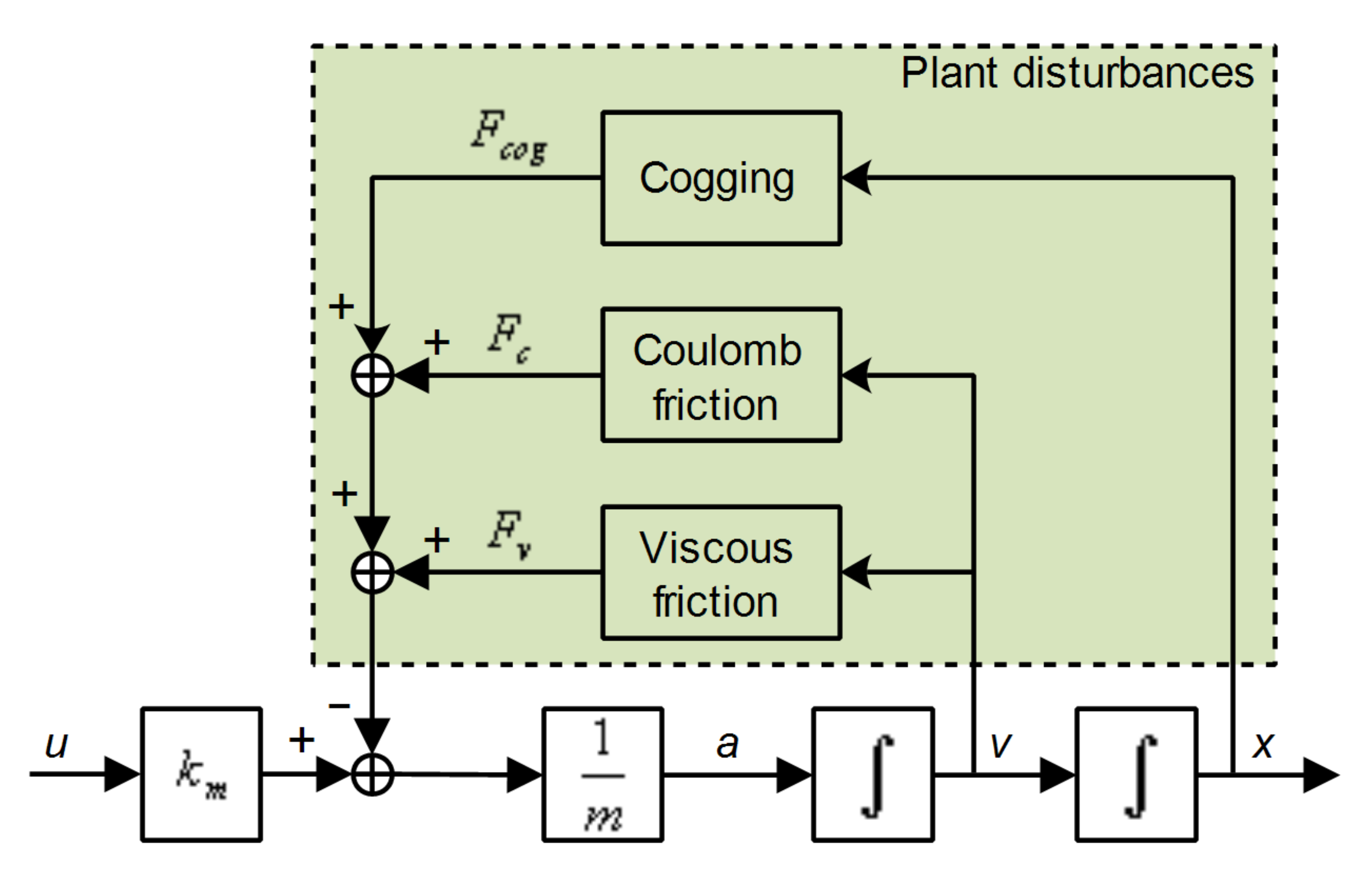
3.1. Simulated Linear Motor

Figure 3 depicts a nonlinear block diagram model of a linear motor that is used as a simulated plant in this case study, where u is the input control signal [V], x, v, and a is the motor position [m], motor velocity [m/s], and motor acceleration [m/s²], respectively. The simulated plant consists of a simple second-order linear model plus nonlinear functions that represent two sources of plant disturbances: (1) the cogging force modeled as a position-dependent disturbance; (2) the coulomb and viscous friction force considered as a velocity-dependent disturbance. These disturbances can be viewed as functions of states of the plant and they have a reproducible characteristic, that is, they are reproduced in the same behavior for each repetitive motion. Parameters of the simulated linear motor are given in

Table 1. Parameters of the simulated linear motor.

Parameter	Value
motor constant $k_m$	69.3
plant mass $m$	10 [kg]
cogging force $F_{cog}=d_{cog}\cdot \sin (1200\cdot x)$	[N]
cogging force magnitude $d_{cog}$	0.1 [N]
coulomb friction $F_c=d_c\cdot \tanh (1000\cdot v)$	[N]
coulomb friction coefficient $d_c$	0.1 [N]
viscous friction $F_v=d_v\cdot v$	[N]
viscous friction coefficient $d_v$	0.2 [Ns/m]

.

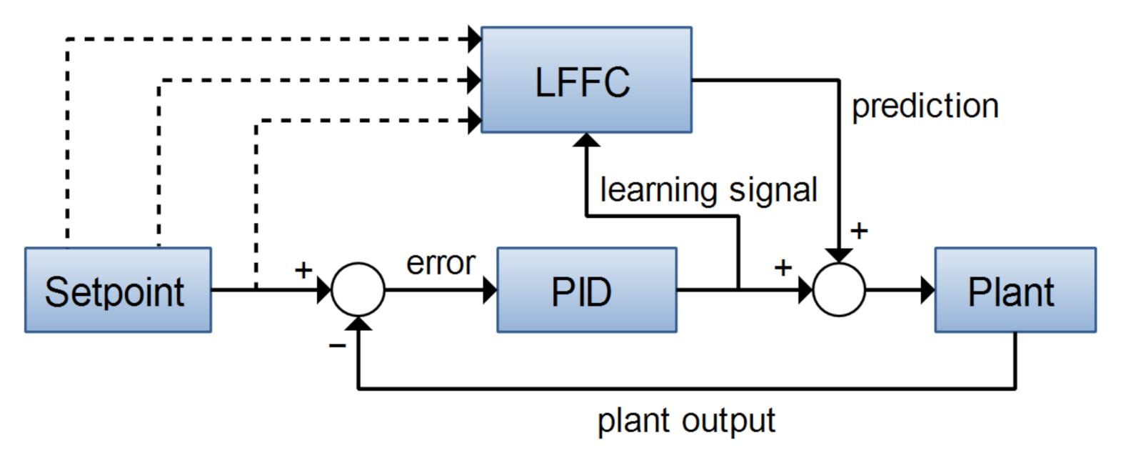
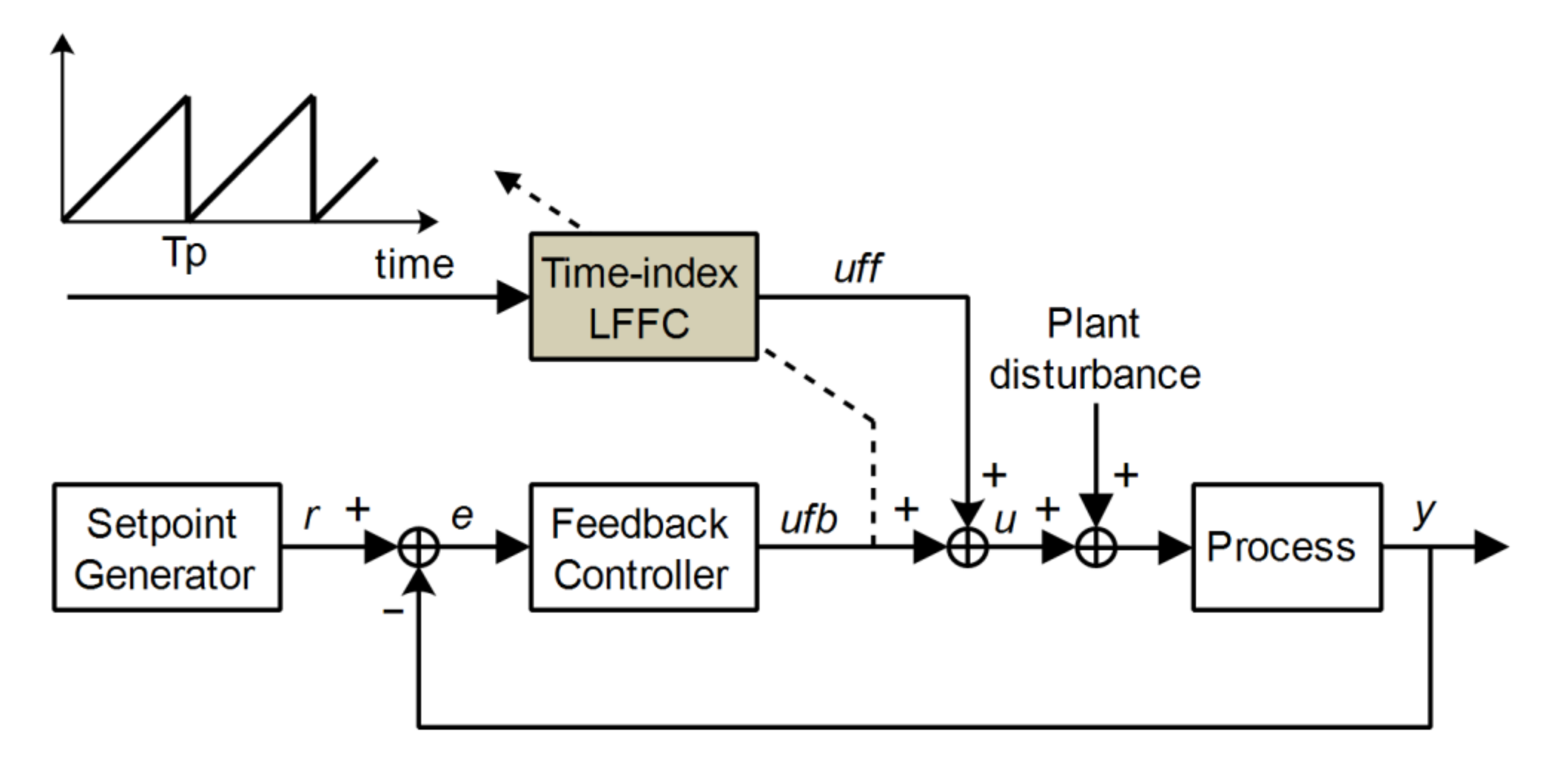
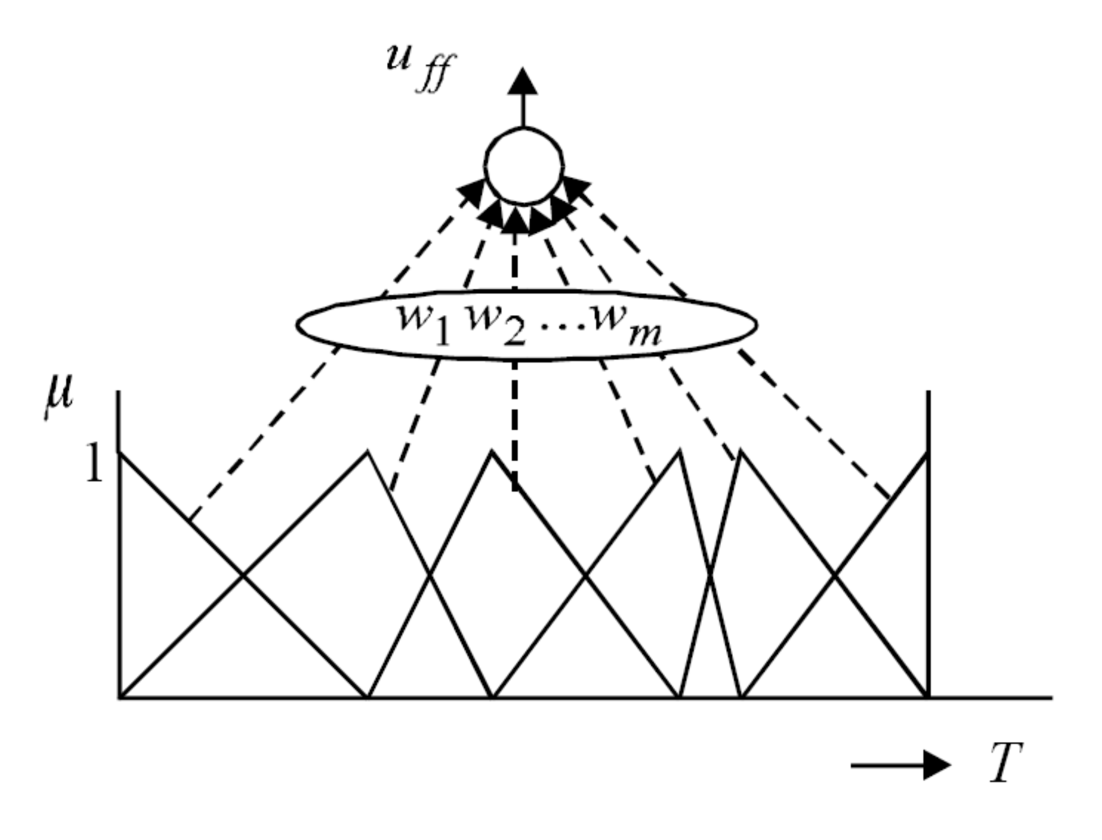
3.2. Design of a Time-Index LFFC

A time-index LFFC system is developed for the simulated linear motor described above. The system consists of a setpoint generator, a feedback controller, and a time-index LFFC that can learn on-line, as shown in Figure 4. In this structure, the output of the feedback controller is used as the learning signal for the time-index LFFC. This means that LFFC learns by minimizing the error of the feedback control signal. Time-index LFFC system is a special kind of LFFC structures in which the desired feedforward signal is a function of the motion time, i.e., t $\in$ [0, T_p], where T_p [s] is the motion time period. This implies that the time-index LFFC can be well applied for repetitive motions. In this case study, the time period of each motion is equal to 6 [s].

When designing a time-index LFFC for a motion control system using linear motor, the feedback controller is designed such that robust stability is guaranteed in the face of model uncertainties; whereas the feedforward controller is designed to compensate for repetitive plant disturbances and to obtain high-performance [1]. In this case study, the feedback control was implemented in the form of a proportional-derivative (PD) controller with the transfer function given by (1). The PD controller was designed with the aim of delivering a robustly stable closed loop system on basis of the second-order linear model (i.e., a moving mass system), which thus has structural errors in comparison with the nonlinear plant model given in Figure 3. Three parameters (K_p = 35.0; T_d = 0.13; β = 0.1) were selected for the PD controller based on tuning rules to obtain safe stability margins. It should be noted that the demand for obtaining a good tracking performance (that is, small position error in the presence of model uncertainties and plant disturbances) is not highly required with regard to the feedback control.

$$\frac{U(s)}{E(s)}=K_p\left(1+\frac{T_{d}s}{\beta T_{d}s+1}\right)$$

(1)

To implement the time-index LFFC, B-spline network (BSN) is used as a function approximator whose input-output mapping can be adapted during control and is intended to become equal to the inverse model of the plant. A BSN is a neural network (NN) that uses B-spline basis functions to approximate an arbitrary (nonlinear) function, i.e., forming a mapping from input to output. A B-spline network of order $n$ consists of piecewise polynomial functions of order $n-1$. In this research, a second-order B-spline neural network is used to generate the feedforward control signal $u_{ff}$ (see Figure 5). The function evaluation of a B-spline is called the membership and is denoted as $\mu$. To create an input-output mapping, B-splines are placed on the domain of the input of the BSN in such a way that at each input value the sum of all memberships is equal to 1. That part of the input space for which $\mu$ is not equal to 0 is called its support [9].

In the time-index LFFC, to realize a mapping from the motion time $t$ to $u_{ff}$ with a BSN, B-splines are placed on the time domain (as shown in Figure 5). The output of the BSN (i.e., $u_{ff}$) at input $t$ is calculated as a weighted sum of the B-spline evaluations as

$$u_{ff}(t)={\displaystyle \sum _{i=1}^m{\mu }_i(t)w_i}$$

(2)

where ${\mu }_i$ is the evaluation of the i-th B-spline, $w_i$ is the weight associated to the i-th B-spline, and $m$ is the number of B-splines.

Training the BSN is done by adjusting the weights of the network. This can be done either online, i.e., after each sample, or offline, i.e., after a specific motion has been completed [1]. In this study, the offline training mode is considered. The learning mechanism according to which the weights of the BSN are adapted at the end of a periodic motion is given in (3) [9]:

$$\Delta w_i=\gamma \frac{{{\displaystyle \sum }}_{k=0}^{T/h}{\mu }_i\left(kh\right)u_{fb}\left(kh\right)}{{{\displaystyle \sum }}_{k=0}^{T/h}{\mu }_i\left(kh\right)}$$

(3)

where $\gamma$ is the learning rate ($0<\gamma <1$), $T$ is the motion time period, $h$ is the sampling time, $u_{fb}$ is the output of the feedback controller, and $\Delta w_i$ is the adaptation of the weight associated to the i-th B-spline.

Finally, as instructed in [1,8,9], the following two important parameters have to be properly specified in the design of the time-index LFFC:

1. The B-spline distribution. The accuracy of the LFFC depends on the width (or support) of the B-splines. Basically, the smaller the width of the B-splines, the more accurate the LFFC. However, a stability analysis [9] showed that B-splines that have a too small width may result in unstable behavior. The minimum width of the B-splines for which the system remains stable can be determined on the basis of a Bode plot of the closed loop transfer function. Specifically, when ${\omega }_{max}$ is the frequency for which the phase shift of the closed loop system exceeds 1.556 [rad] for the first time, the minimum width of the B-splines is given by [1,9]:

$$d_{min}=\frac{2\pi }{{\omega }_{max}}\left[\mathrm{s}\right]$$

(4)

In this study, the minimum width of the B-splines was approximately found as $d_{min}\approx 0.1 \left[\mathrm{s}\right]$. Because the B-splines are placed on the time domain and the time period of each motion is 6 [s], as previously mentioned, it can be interpreted that the number of B-splines should not exceed 60 in order to keep the system remain stable.

2. The learning rate. The learning rate ($0<\gamma <1$) determines how fast the weights of the BSN are adapted. The lower the learning rate, the longer it takes for the tracking error to converge. However, a too high learning rate may result in overshoot and, in the worst case, instability [9]. It is recommended to set $\gamma$ between 0.01 and 0.1.

In this example, a learning rate ($\gamma =0.1$) is used. This learning rate is chosen as a compromise between fast learning and assuring stability.

In summary, the time-index LFFC has been designed such that a small tracking error can be achieved in the presence of model uncertainties as well as plant disturbances. Next, the design of a time-index LFFC in the framework of a multithreaded MACS (i.e., a MACS-based time-index LFFC system) will be described in the following section. To realize the time-index LFFC algorithm, the GNU Scientific Library [39] has been used.

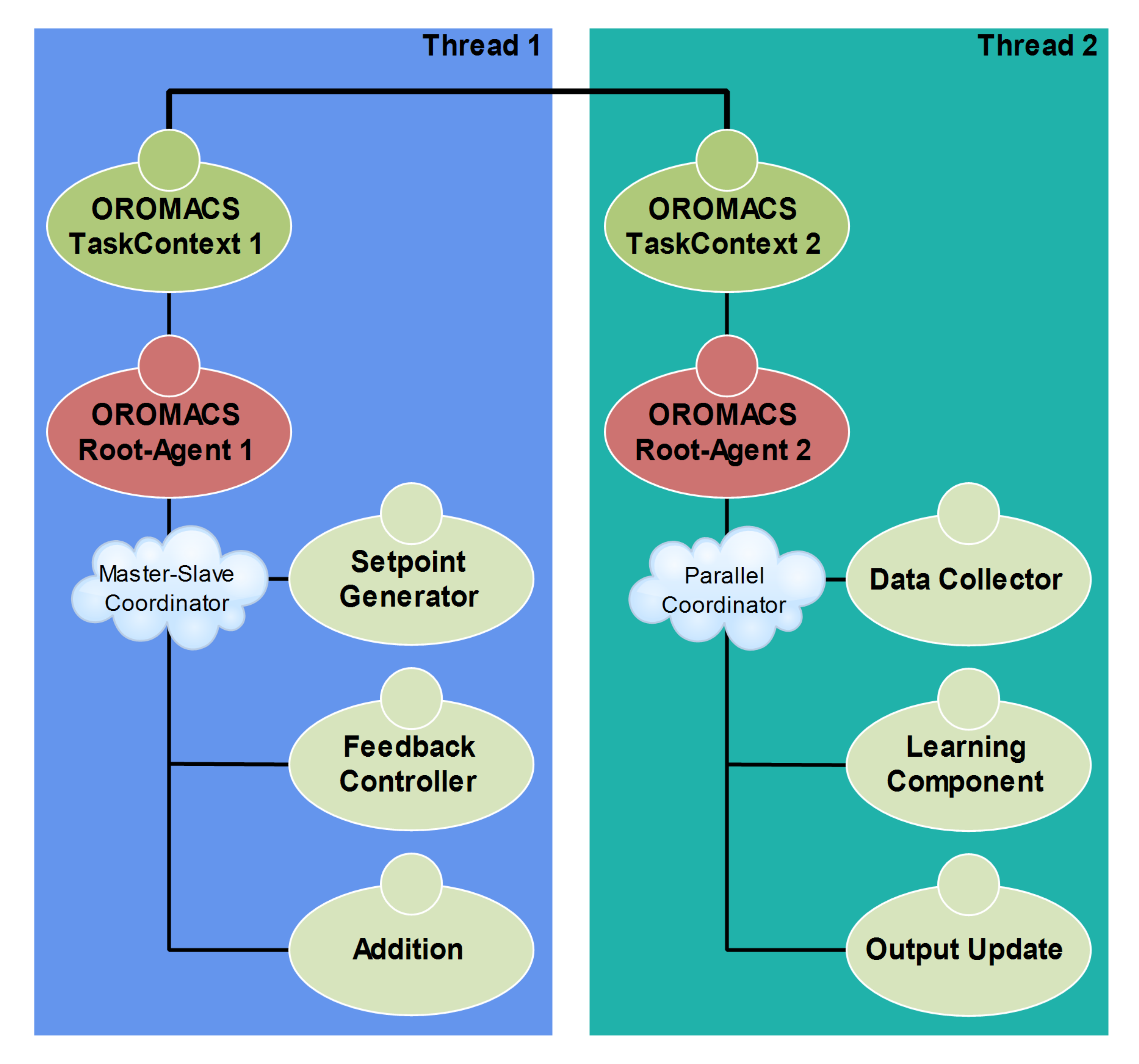
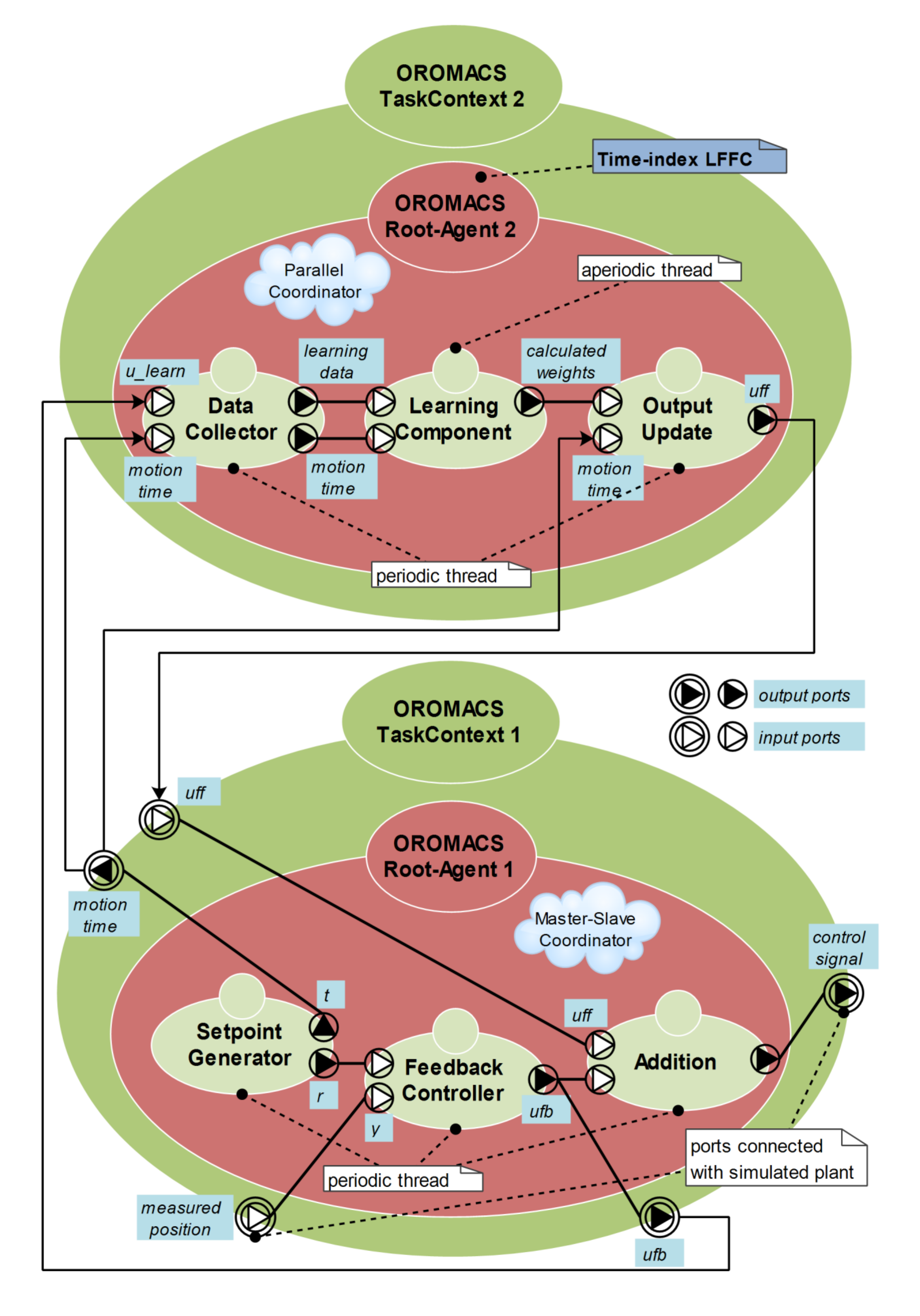
3.3. Design of a MACS-Based Time-Index LFFC System

Using the OROMACS framework [33] we have designed a MACS-based time-index LFFC system for the simulated plant. The hierarchical organization and inside structure of the system is presented in Figure 6 and Figure 7, respectively. The design consists of two OROMACS TaskContexts (TCs) with their missions: OROMACS TC 1 involves the feedback control activity, and OROMACS TC 2 is responsible for the time-index LFFC part. These OROMACS TCs are described in the following.

OROMACS TC 1 contains a composite OROMACS Root-Agent, as shown in Figure 6, which consists of three components: (1) a setpoint generator, (2) a feedback controller, and (3) an addition. These components are real-time periodic tasks running at the same sampling time of T₁ = 1 [ms]. They are coordinated by a master–slave coordinator in which the setpoint generator is the master and the others are the slave. The master–slave coordinator is used in this case due to safety reason, that is, only when the setpoint generator is active and produces the reference position then the feedback controller can be active and produces the control signal. The addition component is used to combine the feedback and feedforward control signal. The setpoint generator also produces motion time that will be used by the time-index LFFC (see Figure 7).

OROMACS TC 2 contains a composite OROMACS Root-Agent, as shown in Figure 6, which consists of three components: (1) a data collector, (2) a learning component, and (3) an output update. These components are coordinated by a parallel coordinator. The data collector and output update components are real-time periodic tasks; whereas the learning component is a non-real-time aperiodic task (as presented in Figure 7). The parallel coordinator makes components in the OROMACS Root-Agent 2 be active concurrently. In other words, these components work/run independently. When a component wants to get active, it gets active, independent of the other components. In the following, these components are described in details.

The data collector is a real-time periodic task running at a sampling time of T₂ = 10 [ms]. As presented in Figure 7, this periodic component is the first part of the time-index LFFC. Its role is to gather data that will be used by the learning component. The collected data are learning signal and motion time, which are provided by the OROMACS TC 1. The learning signal and motion time are received from two input ports u_learn and motion time, respectively. As shown in Figure 7, the feedback control signal is used as the learning signal. In this example, 600 data points are collected at the sampling time of T₂ = 10 [ms]. Hence, it takes 6 [s] to get all data. The collected data points are stored in two vectors and pushed out to the corresponding output ports, i.e., learning data and motion time, as soon as enough data are obtained. Subsequently, the data collector component sends a signal to “wake up” the learning component and concurrently starts collecting new data.

Learning is a non-real-time aperiodic task, which performs the learning feedforward control algorithm. After being “woken up” by the data collector, the learning component starts its computation using 600 data points received from the data collector through two input ports: learning data and motion time. In this example, 32 second-order B-splines are used for the approximation. These B-splines are placed on the time domain, t $\in$ [0, 6] seconds. As soon as the learning process is completed, the results (i.e., weights) are stored in a vector to be sent to the output port calculated weights; and they are immediately made available on the corresponding input port of the output update component of the OROMACS TC 2. Then, the learning component returns to the “sleeping” state and waits for the new 600 data points and “woken-up” signal from the data collector.

Output update is a real-time periodic task running at a sampling time of T₃ = 50 [ms]. As presented in Figure 7, this periodic component is the third part of the time-index LFFC. The role of this output update component is to estimate the feedforward control signal based on the weights calculated by the learning component. The computation results are pushed out to the output port uff, and they are immediately made available on the corresponding input port uff of the OROMACS TC 1. The feedforward and feedback control signal are combined by the addition component to form the total control signal that is used to control the simulated plant.

It should be discussed that it takes 6 [s] for the data collector to collect all 600 data points. Immediately after the data collector completes its first cycle, the learning component is activated and runs. The output update component should start running only after the learning component completes its first computation cycle. As the computation time is unknown and variable in each cycle, a “ready” flag can be used to indicate that the learning component completes its first computation cycle. In this study, a “ready” flag is combined with another condition, i.e., the data collector completes the second data collection cycle, to form the condition to start the output update. This means that the output update will run and produce the feedforward control signal after 12 [s].

Another real-time periodic thread (OROMACS TC 3), which is not presented in Figure 6 and Figure 7, is used for implementing the simulated linear motor with nonlinear disturbances (see Section 3.1). This OROMACS TC contains an elementary OROMACS root-agent, which runs at a sampling time of T₄ = 1 [ms]. Connections between OROMACS TC 1 and OROMACS TC 3 are made through two ports, i.e., measured position and control signal, as shown in Figure 7.

3.4. Discussion

In this study, a MACS-based time-index LFFC system has been designed using two OROMACS TCs. The feedback control activity is designed to run in a real-time periodic thread (OROMACS TC 1), whereas the design of the time-index LFFC part involves three components, running inside OROMACS TC 2, in which the learning algorithm is done on-line, asynchronously, and runs in a non-real-time aperiodic task. The design includes several real-time periodic tasks running at different sampling times, i.e., 1 [ms], 10 [ms], and 50 [ms]. This is possible due to the fact that OROMACS has reused the computation and communication mechanism of the OROCOS framework, therefore data exchange between OROMACS TaskContexts as well as between their components/tasks are deterministic real-time and thread-safe. Also, since OROCOS has fully supported the asynchronous port-based data flow interface between real-time and non-real-time threads [38], OROMACS TaskContexts (and their components/tasks) can run concurrently at different sampling times. It is necessary to mention that multiple sampling times are used in the present work in order to demonstrate that the methodology can be effective even when components/tasks of a control system are required to run at different sampling frequencies (i.e., multirate control systems).

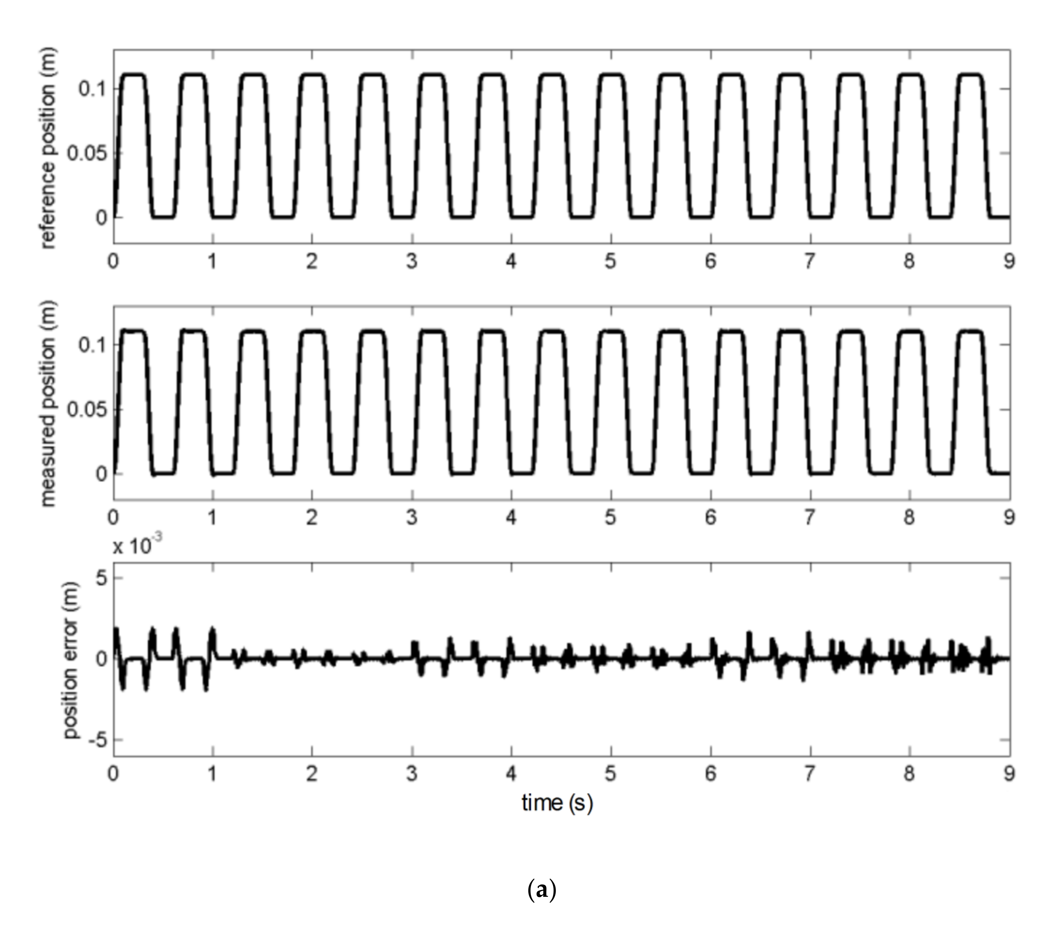
4. Simulation Results

The MACS-based time-index LFFC system, designed in Section 3 for the simulated linear motor with nonlinear disturbances, is simulated using the OROCOS running environment. This is a real-time simulation scheme [38].

The setpoint generator of the OROMACS TC 1 produces fifteen repetitive motions (or strokes), in which each motion goes from the home position at 0 [mm] to the final position at 110 [mm] and then returns back to the home position. These motions (or strokes) are third-order path. As the time period of each motion is 6 [s] so that the simulation time is 90 [s]. The designed MACS-based time-index LFFC system is compared with the case when only feedback control action is used, so as to demonstrate the advantages of the LFFC structure for motion control applications. Besides the cogging and friction force, some mass variations of the plant are used to simulate plant disturbances as follows:

• From t = 0 [s] to 30 [s], the plant mass is 10 kg (initial mass value, see Table 1).
• From t = 30 [s] to 60 [s], the plant mass is increased up to 15 kg.
• From t = 60 [s] to 90 [s], the plant mass is increased up to 20 kg.

In the feedback control loop, the parameters (K_p = 35.0; T_d = 0.13; β = 0.1) are assigned for the PD controller. Regarding the time-index LFFC, 32 second-order B-splines are used for the approximation. These B-splines are placed on the time domain t $\in$ [0, 6] seconds where 600 data points are used in each learning cycle.

The first test is performed when the simulated plant is the second-order linear model without the effect of nonlinear cogging and friction force. During the first two cycles (from t = 0 [s] to 12 [s]) when only the feedback controller is used, the position error is large; its maximum value is about 2 [mm]. However, after the learning and output update components of the time-index LFFC are active and produce the feedforward control action, the position error is considerably reduced, as shown in Figure 8a. At t = 30 [s] and t = 60 [s] when the plant mass is increased, the position error becomes rather larger. However, the position error decreases rapidly after two learning cycles. Figure 8b shows that the feedforward control action has a tendency to be larger to compensate for the increase of the plant mass.

The second test is performed when the simulated plant is the second-order linear model in the presence of nonlinear cogging and friction force. During the first two cycles (from t = 0 [s] to 12 [s]) when only the feedback controller is used, as the nonlinear disturbances are added to the plant, the tracking performance are significantly declined in comparison with the first test; the maximum position error increases from 2 [mm] to more than 5 [mm], as presented in Figure 9a. However, after the feedforward control action is activated, the position error reduces quickly. These results have proved that the use of MACS-based LFFC can improve not only the disturbance rejection, but also the stability robustness of the controlled system. Figure 9b reveals that the effect of nonlinear cogging and friction force causes a noiselike behavior in the feedback control signal. Also, as similar to the first test, the feedforward control signal has a tendency to increase to compensate for the increase of the plant mass.

5. Conclusions and Further Discussion

This paper has presented a novel MACS-based time-index LFFC design method for mechatronic systems. To the best of the author’s knowledge, integrating LFFC into the framework of MACS is reported for the first time by the present work. Based on this approach, the feedback control part is realized in a real-time periodic MACS, while the time-index LFFC algorithm can be deployed on-line, asynchronously, and in a separate non-real-time aperiodic MACS. Simulation results of the MACS-based time-index LFFC system developed for the simulated linear motor have demonstrated the applicability of the design method. The reproducible disturbances and mass variations have been successfully compensated by the time-index LFFC algorithm using a second-order B-spline neural network.

Using the MACS-based design approach, the time-index LFFC system is divided into several simple control components, which are coordinated by coordinators. This component-based design method brings many advantages, such as the development time can be reduced and the reliability of the developed control system can be increased. Also, in case if a particular part of the control system (e.g., LFFC or feedback controller) requires to be modified, one just needs to modify the required part, without redesigning and/or reprogramming the entire control system.

To provide real-time features, development and runtime environment for MACS-based control systems, one may directly use the application programming interface (API) and system services of a real-time operating system (RTOS), such as timer functions, event management, task communication methods (semaphores, queues, and mailboxes), memory management, interrupt handlers and the scheduler, etc. This low-level software programming approach requires designers with high embedded system development skills. Also, using the powerful but dangerously unstructured API of an RTOS can make designers miss the possibility to develop more structured, deterministic and portable control software systems [40]. Hence, it is argued that MACS-based control systems should be relied on an established component-based software framework that can provide essential features, such as deterministic real-time thread-safe behavior, task management and scheduling tools, interprocess communication mechanism with lock-free data exchange, capability to handle discrete-events in both synchronous and asynchronous way, and other useful features. For this reason, the OROCOS framework has been used as the development and runtime environment in this study.

Since the main focus of this work is to present and demonstrate the applicability of the MACS-based advanced control system design approach (in particular, a MACS-based time-index LFFC design method), a simulated linear motor has been used in this paper in a simulation scheme. More complex setups, including real-life and industrial applications, will be definitely used to validate the proposed method in the future. Also, it is anticipated that the proposed approach would be also useful for other advanced control architectures, such as nonlinear model predictive control, neural-network-based control, nonlinear model reference adaptive control, etc. Therefore, a potential future work is to consider applying the approach for these advanced control architectures.

References

1. Velthuis, W.J.R. Learning Feedforward Control: Theory, Design and Applications. Ph.D. Thesis, University of Twente, Enschede, The Netherlands, 2000. [Google Scholar]
2. Astrom, K.J.; Wittenmark, B. Adaptive Control; Addison-Wesley: Boston, MA, USA, 1995. [Google Scholar]
3. Babuška, R.; Damen, M.R.; Hellinga, C.; Maarleveld, H. Intelligent adaptive control of bioreactors. J. Intell. Manuf. 2003, 14, 255–265. [Google Scholar] [CrossRef]
4. Tan, C.; Tao, G.; Qi, R.; Yang, H. A direct MRAC based multivariable multiple-model switching control scheme. Automatica 2017, 84, 190–198. [Google Scholar] [CrossRef]
5. Jang, T.J.; Choi, C.H.; Ahn, H.S. Iterative learning control in feedback systems. Automatica 1995, 31, 243–245. [Google Scholar] [CrossRef]
6. Verwoerd, M. Iterative Learning Control: A Critical Review. Ph.D. Thesis, University of Twente, Enschede, The Netherlands, 2005. [Google Scholar]
7. Liu, L.; Tian, S.; Xue, D.; Zhang, T.; Chen, Y.Q. Industrial feedforward control technology: A review. J. Intell. Manuf. 2019, 30, 2819–2833. [Google Scholar] [CrossRef]
8. Otten, G.; De Vries, T.J.A.; Van Amerongen, J.; Rankers, A.M.; Gaal, E.W. Linear motor motion control using a learning feedforward controller. IEEE ASME Trans. Mechatron. 1997, 2, 179–187. [Google Scholar] [CrossRef] [Green Version]
9. Velthuis, W.J.R.; De Vries, T.J.A.; Schaak, P.; Gaal, E.W. Stability analysis of learning feed-forward control. Automatica 2000, 36, 1889–1895. [Google Scholar] [CrossRef]
10. De Vries, T.J.A.; Velthuis, W.J.R.; Idema, L.J. Application of parsimonious learning feedforward control to mechatronic systems. IEE Proc. Control Theory Appl. 2001, 148, 318–322. [Google Scholar] [CrossRef]
11. Chen, Y.; Moore, K.L.; Bahl, V. Learning feedforward control using a dilated B-spline network: Frequency domain analysis and design. IEEE Trans. Neural Netw. 2004, 15, 355–366. [Google Scholar] [CrossRef]
12. Van Amerongen, J. A MRAS-based Learning Feed-forward Controller. In Proceedings of the 4th IFAC Symposium on Mechatronic Systems, Heidelberg, Germany, 12–14 September 2006; Volume 39, pp. 758–763. [Google Scholar]
13. Lin, Z.; Wang, J.; Howe, D. A learning feed-forward current controller for linear reciprocating vapor compressors. IEEE Trans. Ind. Electron. 2011, 58, 3383–3390. [Google Scholar] [CrossRef]
14. Lee, F.S.; Wang, J.C.; Chien, C.J. B-spline network-based iterative learning control for trajectory tracking of a piezoelectric actuator. Mech. Syst. Signal Process. 2009, 23, 523–538. [Google Scholar] [CrossRef]
15. Deng, H.; Oruganti, R.; Srinivasan, D. Neural controller for UPS Inverters based on B-spline network. IEEE Trans. Ind. Electron. 2008, 55, 899–909. [Google Scholar] [CrossRef]
16. Zhao, Y.; Li, Y.; Dehghan, S.; Chen, Y.Q. Learning feedforward control of a one-stage refrigeration system. IEEE Access 2019, 7, 64120–64126. [Google Scholar] [CrossRef]
17. Sprunt, B.; Sha, L.; Lehoczky, J. Aperiodic task scheduling for hard-real-time systems. Real. Time Syst. 1989, 1, 27–60. [Google Scholar] [CrossRef]
18. Lin, T.H.; Tarng, W. Scheduling periodic and aperiodic tasks in hard real-time computing systems. In Proceedings of the ACM SIGMETRICS Conference on Measurement and Modeling of Computer Systems, San Diego, CA, USA, 21–24 May 1991; pp. 31–38. [Google Scholar]
19. Spuri, M.; Buttazzo, G. Scheduling aperiodic tasks in dynamic priority systems. Real. Time Syst. 1996, 10, 179–210. [Google Scholar] [CrossRef]
20. Park, S.J.; Yang, J.M. Supervisory control for real-time scheduling of periodic and sporadic tasks with resource constraints. Automatica 2009, 45, 2597–2604. [Google Scholar] [CrossRef]
21. Buttazzo, G.C. Hard Real-Time Computing Systems: Predictable Scheduling Algorithms and Applications; Real-Time Systems Series; Springer: Boston, MA, USA, 2011; Volume 24. [Google Scholar]
22. Johansen, T.A.; Murray-Smith, R. The Operating Regime Approach to Nonlinear Modelling and Control. In Multiple Model Approaches to Modelling and Control; Murray-Smith, R., Johansen, T.A., Eds.; Taylor and Francis: London, UK, 1997; pp. 3–72. [Google Scholar]
23. Pagès, O.; Caron, B.; Ordónez, R.; Mouille, P. Control system design by using a multi-controller approach with a real-time experimentation for a robot wrist. Int. J. Control 2002, 75, 1321–1334. [Google Scholar] [CrossRef]
24. Leitão, P. Agent-based distributed manufacturing control: A state-of-the-art survey. Eng. Appl. Artif. Intell. 2009, 22, 979–991. [Google Scholar] [CrossRef]
25. Ribeiro, L.; Barata, J. Deployment of Multiagent Mechatronic Systems. In Industrial Applications of Holonic and Multi-Agent Systems; Lecture Notes in Computer, Science; Mařík, V., Lastra, J.L.M., Skobelev, P., Eds.; Springer: Berlin/Heidelberg, Germany, 2013; Volume 8062, pp. 71–82. [Google Scholar]
26. Farid, A.M.; Ribeiro, L. An axiomatic design of a multi-agent reconfigurable mechatronic system architecture. IEEE Trans. Ind. Inform. 2015, 11, 1142–1155. [Google Scholar] [CrossRef] [Green Version]
27. Leitão, P.; Karnouskos, S.; Ribeiro, L.; Lee, J.; Strasser, T.; Colombo, A.W. Smart agents in industrial cyber-physical systems. Proc. IEEE 2016, 104, 1086–1101. [Google Scholar] [CrossRef] [Green Version]
28. Qin, J.; Ma, Q.; Shi, Y.; Wang, L. Recent advances in consensus of multi-agent systems: A brief survey. IEEE Trans. Ind. Electron. 2017, 64, 4972–4983. [Google Scholar] [CrossRef]
29. Sahnoun, M.; Baudry, D.; Mustafee, N.; Louis, A.; Smart, P.A.; Godsiff, P.; Mazari, B. Modelling and simulation of operation and maintenance strategy for offshore wind farms based on multi-agent system. J. Intell. Manuf. 2019, 30, 2981–2997. [Google Scholar] [CrossRef] [Green Version]
30. Jiménez, A.C.; García-Díaz, V.; Castro, S.J.B. A decentralized framework for multi-agent robotic systems. Sensors 2018, 18, 417. [Google Scholar] [CrossRef] [Green Version]
31. Maoudj, A.; Bouzouia, B.; Hentout, A.; Kouider, A.; Toumi, R. Distributed multi-agent scheduling and control system for robotic flexible assembly cells. J. Intell. Manuf. 2019, 30, 1629–1644. [Google Scholar] [CrossRef]
32. Fan, Y.; Chen, J.; Song, C.; Wang, Y. Event-triggered coordination control for multi-agent systems with connectivity preservation. Int. J. Control Autom. Syst. 2020, 18, 966–979. [Google Scholar] [CrossRef]
33. Dao, P.B. OROMACS: A design framework for multi-agent control system. Int. J. Control Autom. Syst. accepted for publication. [CrossRef]
34. The Open Robot Control Software (OROCOS) Project. Available online: http://www.orocos.org/ (accessed on 26 July 2020).
35. Rezola, I. Learning Multi-Agent Control with OROCOS. Master’s Thesis, University of Twente, Enschede, The Netherlands, 2009. [Google Scholar]
36. Bruyninckx, H. Open robot control software: The OROCOS Project. In Proceedings of the IEEE International Conference on Robotics and Automation (ICRA), Seoul, Korea, 21–26 May 2001; pp. 2523–2528. [Google Scholar]
37. Bruyninckx, H.; Soetens, P.; Koninckx, B. The Real-time Motion Control Core of the Orocos Project. In Proceedings of the IEEE International Conference on Robotics and Automation (ICRA), Taipei, Taiwan, 14–19 September 2003; pp. 2766–2771. [Google Scholar]
38. OROCOS Component Builder’s Manual. Available online: https://www.orocos.org/stable/documentation/rtt/v2.x/doc-xml/orocos-components-manual.html (accessed on 26 July 2020).
39. GNU Scientific Library. Available online: http://www.gnu.org/software/gsl/ (accessed on 10 July 2020).
40. Bruyninckx, H. Real-Time and Embedded Guide; Katholieke Universiteit Leuven: Leuven, Belgium, 2002. [Google Scholar]
Figure 1. Basic scheme for a learning feedforward controller.
Energies 14 00420 g001
Figure 2. Hierarchically structured multiagent control system (MACS) using the controller-agent-based design framework OROMACS.
Energies 14 00420 g002
Figure 3. Nonlinear block diagram model of the simulated linear motor.
Energies 14 00420 g003
Figure 4. Control system based on time-index learning feedforward control (LFFC) and feedback control.
Energies 14 00420 g004
Figure 5. Approximation of the feedforward control signal using a second-order B-spline neural network (BSN).
Energies 14 00420 g005
Figure 6. Hierarchical organization of the MACS-based time-index LFFC system.
Energies 14 00420 g006
Figure 7. Inside structure of the designed MACS-based time-index LFFC system.
Energies 14 00420 g007
Figure 8. The first test without the effect of nonlinear cogging and friction force: (a) position error; (b) control signal.
Energies 14 00420 g008aEnergies 14 00420 g008b
Figure 9. The second test with the effect of nonlinear cogging and friction force: (a) position error; (b) control signal.
Energies 14 00420 g009aEnergies 14 00420 g009b