Abstract
In this paper, we study the dynamics of a two-degree freedom system consisting of the main body and tuned mass damper with inerter (TMDI). We add the dash-pot with variable damping coefficient to TMDI to study the overall efficiency of the device. We investigate different types of the non-linear characteristic of the dash-pot. We investigate devices in which damping coefficient change according to the relative displacement or the relative velocity between the damped mass and tuned mass damper. We also include in the investigation of different types of control functions. We show the two-parameter diagrams presenting the main body’s maximum amplitude versus the frequency of excitation of the damped body and different control parameter. We show how the application of a non-linear damper lets us control the main system’s oscillation amplitude.
1. Introduction
Vibrations of machines and structures under external excitation are usually unwanted. Thus, attempts to design devices that mitigate these oscillations. The first simple solution was tuned mass damper (TMD) proposed by Farhm in 1909 [1] and modified by Den Hartog in 1934 [2]. The classical TMD consists of a mass attached to the damped system via linear spring and damper. Its natural frequency has to be tuned to the natural frequency of the damped body; hence, it damps out vibrations of the main body close to the one selected resonance. The span of frequency where we observe a significant decrease in the amplitude dependents on damping coefficient of the TMD dash-pot. When it is equal to zero, the amplitude of the main body drops down to zero for resonant frequency, but TMD is effective in the very narrow frequency range close to the resonance. The increase in damping coefficient increases the effective range of mitigation of oscillations, but the amplitude of the main body is no longer zero in the resonance. Den Hartog [2] proposed a method to calculate the optimum value of damping coefficient of the TMD dash-pot. However, even in the optimized case, we still observe a significant increase in the main body oscillations amplitude around the resonance frequency.
Nowadays, there are a lot of strategies to increase the effectiveness of TMDs [3,4,5,6,7,8,9,10]. We can divide TMDs into three main groups—i.e., passive, semi-active, or active devices. While the first case is the simplest and the most reliable one, we meet many obstacles due to which its applicability is limited. The semi-active and active devices have a much wider area of application. Another possibility is to expand the TMD with an inerter (TMDI) to extend its efficiency. Inerter is a mechanical device generating force proportional to the relative acceleration of its ends—i.e., [11,12,13,14]. Initially, inerters [15] were successfully applied in sports cars’ suspensions [11,16]. Now, we observe growing number of studies on possible applications including: railway vehicles’ suspensions [17,18,19], devices that absorb impact forces [20] or mitigate vibrations of structures [21,22,23,24,25,26,27,28]. In our previous papers, we examine the TMDI [29,30,31,32] which enables changes of inertance. Hence, the natural frequency of TMDI can be tuned to the frequency of excitation.
This work is devoted to the examination of the efficiency of the TMDI with fixed inertance and non-linear dash-pot. The mass of the TMDI is split between the real mass of the moving body and the inertance. Hence, the TMDI is much lighter than classical TMD with the same damping abilities. We use the non-linear dash-pot, whose damping function depends on a control parameter and the relative displacement or the velocity between the TMDI and the damped body. We show how such a dash-pot influences the mitigation properties of the TMDI using different types of damping functions. All parameters of the system used in this study are taken from our laboratory rig [31]; hence, it also provides us with important information that can be used in the future development of our experimental device. In our previous paper [33] we presented the preliminary results about the configuration of the system considered in this paper. We showed there were just two out of eight considered cases of the dash-pot control functions, but to have clarity and complete view on the introduced idea of control, we decide to present all investigated possibilities here. In the literature, there are a few attempts of analysis of TMDI with a non-linear dash-pot. In [34], the authors consider features of a fluid inerter device for optimized structural control of buildings. The model of the proposed inerter includes in parallel with the inerter itself a non-linear dash-pot representing a power-law damping term. It is shown that the application of a fluid inerter for base-isolation of structures causes a significant decrease in the system amplitude. There are also studies on classical TMD with non-linear dash-pot with piecewise characteristic [35,36] or hardening type function [37]. The authors assume that damping coefficient changes when the relative velocity between the structure and the TMD grows. It is shown that in the case of seismic or wind excitation, such an approach gives good results.
The paper is organized as follow: In Section 2 we describe the model of the analyzed system. The methodology of investigation is described in Section 3. The reference response of TMDI with linear damping function is shown and described in Section 4. Section 5 and Section 6 include the results for dampers with non-linear damping characteristics given by continuous and piecewise functions. Finally, we summarize and conclude our work in Section 7.
2. The Model of the Tuned Mass Damper with Inerter and Non-Linear Dash-Pot
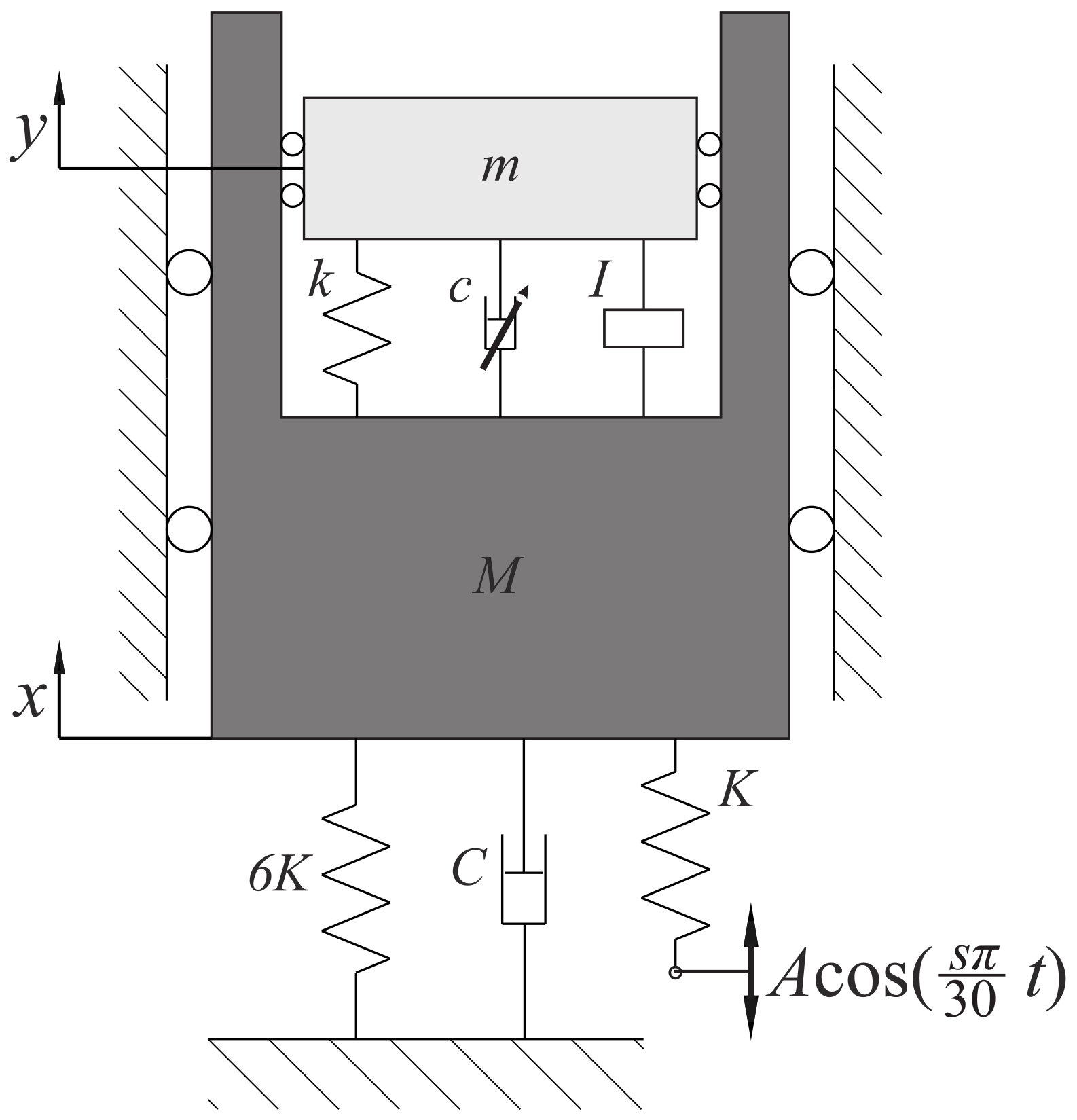
In this section, we describe the mathematical model of the system presented in Figure 1. The model has two degrees of freedom and consists of two coupled oscillators that can move in the vertical direction. The first one serves as a model of the main oscillator, which motion should be mitigated. It is connected with the support and forced via kinematic excitation. The second oscillator is connected to the first one and represents the TMDI. It is connected with the main oscillator via linear spring, non-linear damper and inerter. In this paper, we use the model based on an experimental rig designed and built in our laboratory [30].
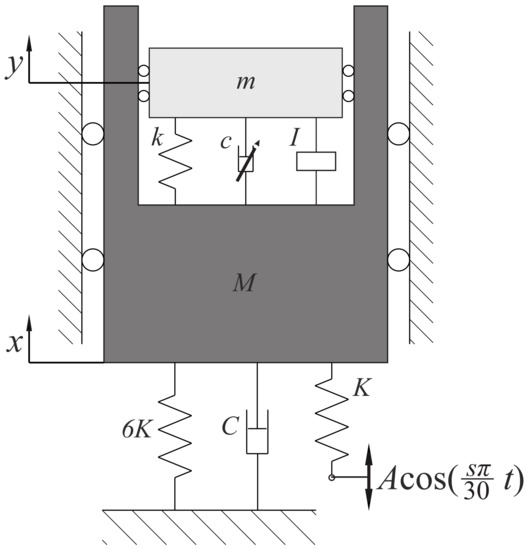
Figure 1.
Model of the system.
Two generalized coordinates describe the motion of the system: the position of the main oscillator by coordinate x, while the displacement of the TMDI by coordinate y. The main oscillator is characterized by the following parameters: M is its mass, K is the stiffness of the single spring that connects the main mass to the ground (we use six such springs), and C is the viscous damping coefficient of the dash-pot that links mass M and the support. Formula expresses the kinematic excitation of the main oscillator with the frequency that corresponds to the speed of the forcing servomotor and the crank on the exciting plate set to A. During the investigation we analyze the response of the structure for fixed crank and different frequencies of excitation that correspond to the following range of rotational speeds: . The kinematic exaction is imposed via spring with a stiffness coefficient K.
To characterize TMDI, we use the following parameters: the moving mass is given by m, the stiffness of the spring that connects it to the main oscillator is described with a parameter k. The non-linear damping function of the dash-pot that connect mass m with M is given by function and the constant interface is given by parameter I.
Using the Lagrange equations of the second kind, we derived the equations of motion of the system presented in Figure 1. After simplification, the equations of motion can be written as follows:
where values of parameters are as follow: , , , , , and Damping function will be defined in the next section.
3. Methodology
In the paper, we investigate if, by control of viscous damping coefficient, it is possible to improve the damping efficiency of the tuned mass damper with the inerter. In the above sections, we describe the concept of the device with a controllable damping coefficient and its mathematical model that is under consideration. We assume that the controllable dash-pot enables us to achieve all values of damping coefficient from the range and we consider two different strategies of control of the viscous damping coefficient c.
The first strategy is named strategy 0, and is described in Section 4. In strategy 0, we assume that damping coefficient value is adjusted to the current frequency of excitation and it stays fixed until the excitation changes. Such an approach is simple and does not require fast changes in damping coefficient value. Then, we assume that damping coefficient can vary during operation for a fixed frequency. We investigate 8 different functions that describe changes in damping coefficient based on the displacement or velocity of the tuned mass damper. In Table 1 we present the diagram explaining the underlying methodology of investigation, and all considered control functions.

Table 1.
Explanation of the investigation methodology and considered control functions.
We analyze both non-linear continuous and piecewise linear functions which increase or decrease the value of damping coefficient basing on the actual displacement or velocity of the damper with respect to the damped mass M. Numbers in brackets, given in Table 1, are used to identify the strategies. Each considered function has three parameters: , that refer to the maximum and minimum achievable value of damping coefficient, and a that defines when (for piecewise linear case) or how sudden (for non-linear) c is changed. During investigation, we assume fixed values of and and change the value of a to give a better overview of the effects on the applied control function. Results are shown using color maps that reflect the amplitude of the system, which we supplement with frequency response curves, showing the response of the structure for given a values.
Of course, there is an infinite number of different functions that could be considered, but with the proposed methodology, we cover a wide range of control strategies. Thus, the obtained results lead us to general conclusions on the influence of variable damping coefficient on the efficiency of TMDI.
4. The Influence of Fixed Damping Coefficient—Strategy 0
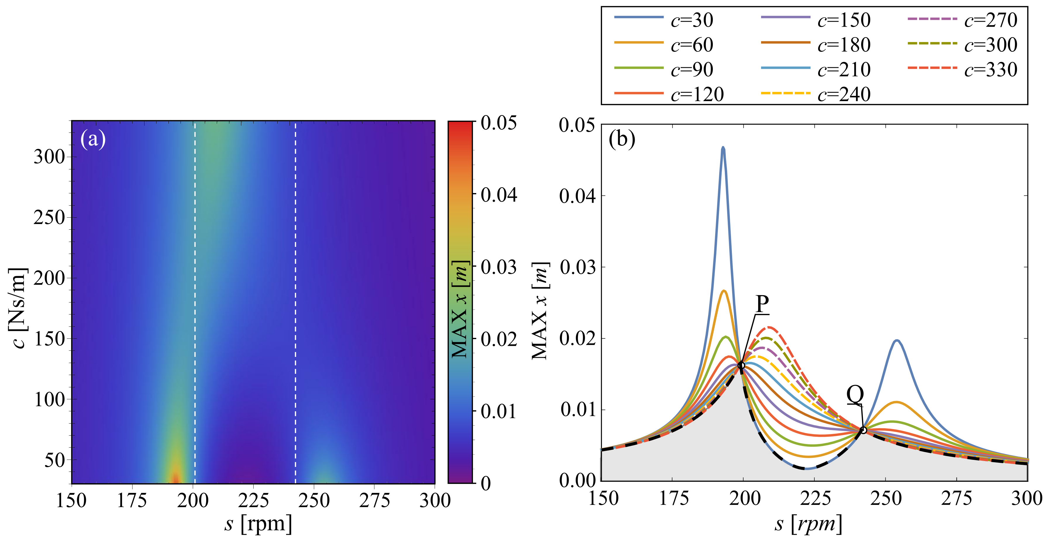
In this section, we study strategy 0, which refers to the response of the linear system with changes of viscous damping coefficient c. We presented obtained results in Figure 2 using a color map (a) and frequency response curves (b). The plots are calculated numerically with Auto07p. We divide the range of parameter c into 100 steps, and for each, we compute the frequency response curve. The blue color corresponds to low amplitude, and it dominates in the plot. The increase in amplitude is observed in the neighborhood of resonances. For low value of damping two resonances occur for and . For the maximum value we observe one resonance for . The transition is caused by the increase in the value of damping coefficient, which causes the stiffening of the connection between the main body and damper. Hence, the independent motion of the TMDI is no more possible, and the system is reduced to one DoF.

Figure 2.
Effectiveness of strategy 0. The plot shows the influence of damping coefficient value on the response of the system. In panel (a) we show two dimensional plot of maximum amplitude of damped system () in two parameters of space: a and s. The panel (b) refers to eleven exemplary FRCs of the damped system.
The corresponding FRCs are shown in Figure 2b for 11 values of damping coefficients, starting with and step . The amplitude of the second resonance is decreasing rapidly, and finally, for , the increase in amplitude is not more present. As it is well known, all FRCs are crossing two points: and , where the response of the system is nearly independent of the value of damping coefficient. The location of those points can be shifted only by changing the natural frequency of the TMDI or via the destabilization of periodic solutions.
Analyzing the plots, we see that assuming strategy 0, one should apply minimum value of damping coefficient for frequencies of excitation below point P and above point Q, namely for and maximum value of damping coefficient between points P and Q, namely for excitation Then, one can obtain the response of the system that is marked with the black dashed line. Gray color marks the area below this curve and will be the benchmark for further investigation. This curve also corresponds to the bang–bang control scenario, wherein the range between points P and Q damping coefficient is changed from minimum to maximum value.
5. Non-Linear Continuous Damping Function—Strategies 1, 2, 3, 4
In this section, we analyze control strategies, assuming non-linear continuous damping functions; namely, strategies 1, 2, 3 and 4. The damping function depends on the retaliative displacement (strategy 1 and 3) or velocity (strategy 2 and 4) between the main system and the TMDI. For the sake of generality, we include all state variables in the general form of damping function. In each case, we consider the increase or the decrease in damping coefficient and investigate the response for different values of parameter a that describes the rate of c change. The system is smooth, hence we perform all calculations in Auto07p.
First, we consider strategy 1 that refers to the following function:
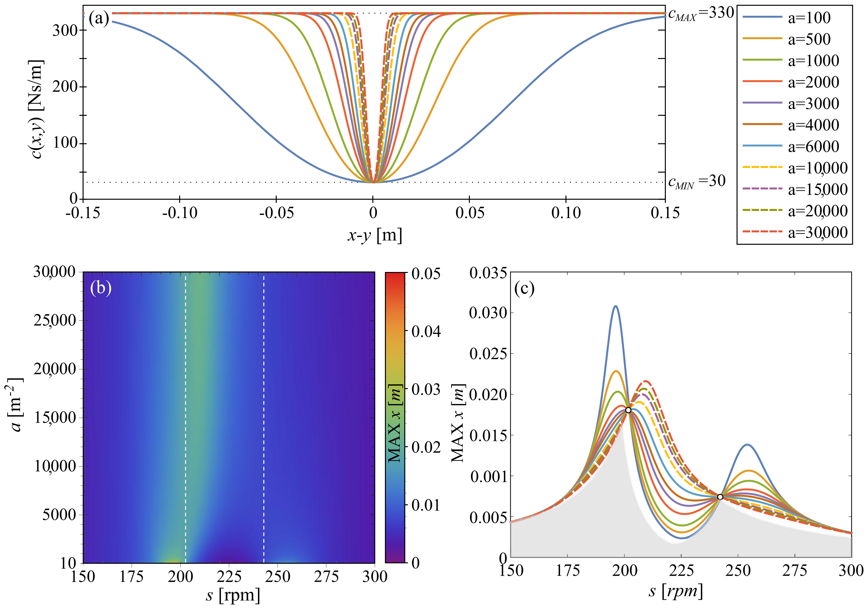
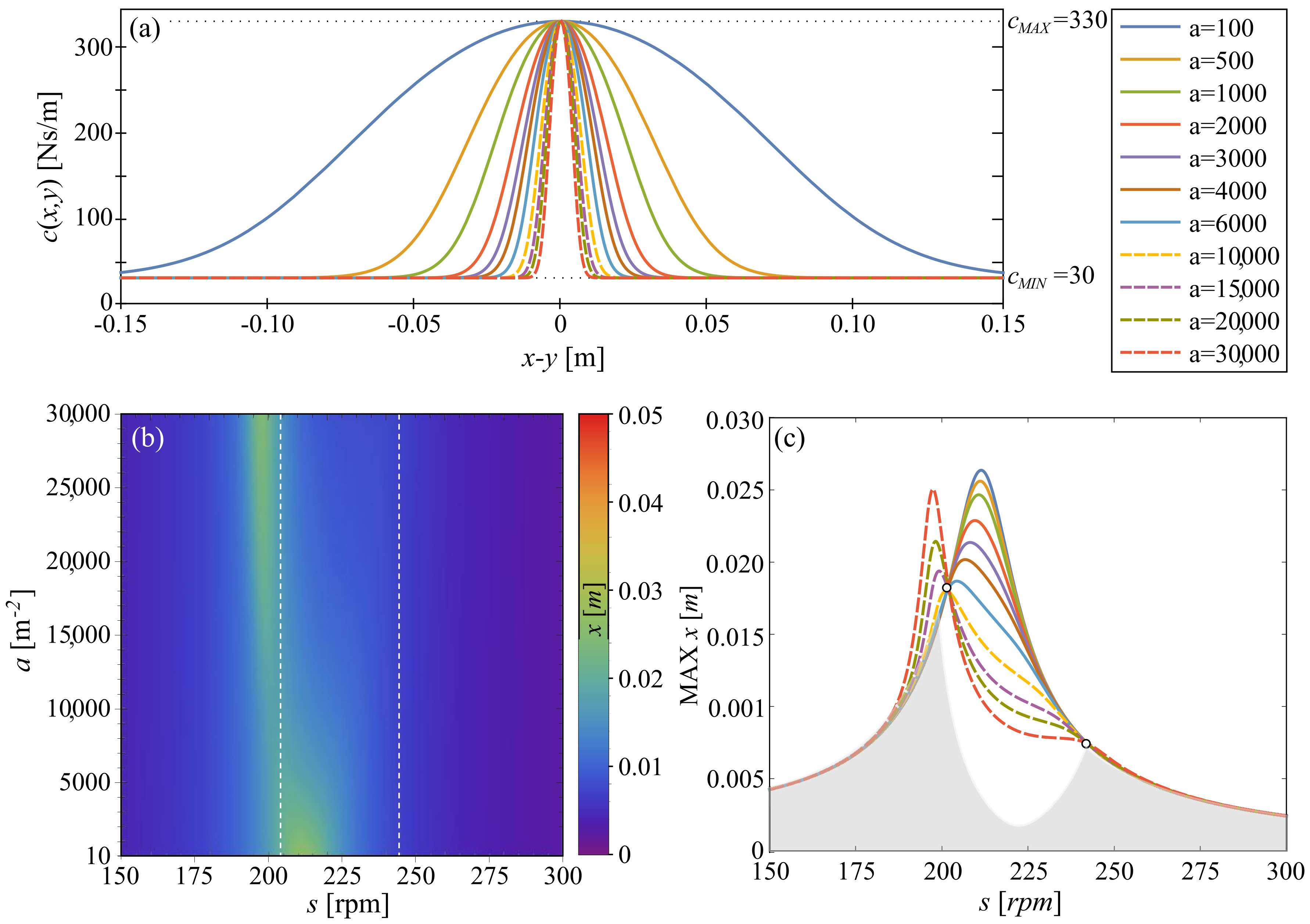
The controlling parameter of the damping function a can vary in range which lets us change the value of relative displacement for which the function achieves its maximum. Regardless of a value, when , the damping coefficient has its minimal possible value . In Figure 3a, ten exemplary plots show how the value of a influences the rate of c change. We restricted the range to because in the considered system, the system is always within this range.

Figure 3.
In panel (a) we show the damping functions (Equation (3)) for selected values of a. In panel (b) we show two dimensional plot of maximum amplitude of damped system () in two parameters of space: a and s. The last panel (c) shows eleven exemplary FRCs of the damped system.
Results are shown in Figure 3b,c. In panel (a) we present a two-dimensional color plot of maximum amplitude of the main system as a function of rotational speed s (frequency of excitation) and parameter of damping function a. White dash lines indicate the location of points [rpm] and [rpm] for the system with linear viscous damping. In Figure 3c we show eleven exemplary FRCs for equally spaced values of parameter a within the considered range. As it is easy to see, the location of points P and Q change only slightly when we apply strategy 1, while the FRCs are significantly different. For a low value of a, we observe two resonances and for the maximum value of a, the main mass and TMDI behave like one DoF system. In Figure 3, with gray color we show the area below the optimum FRC achieved using strategy 0. We see that strategy 1 does not help to improve the TMDI effectiveness over strategy 0, which is much more simple.
Next, we consider case 2 for which we use the following function:
where parameter a in this case is in the range . Ten exemplary plots of the above function are shown in Figure 4a and, as in the previous case, the value of a is governing the slope of the function.
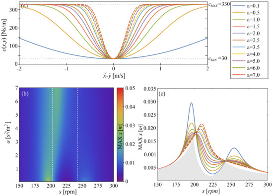
Figure 4.
In panel (a) we show the damping functions (Equation (4)) for selected values of a. In panel (b) we show two dimensional plot of maximum amplitude of damped system () in two parameters space: a and s. The last panel (c) shows eleven exemplary FRCs of damped system.
The corresponding two-dimensional color plot of amplitude versus rotational speed of the servomotor and parameter a is shown in Figure 4b. The dashed white lines indicate the position of points P and Q. With the increase in parameter a, the system is tending to behave like a one DoF system. All periodic solutions are stable, and locations of points P and Q along the FRC are barely affected by non-linear damping (see Figure 4c). Comparing the results with the gray area, which shows what can be achieved with strategy 0, we see that strategy 2 is less appropriate.
After considering strategies 1 and 2 in which the value of c increases, we proceed to strategies 3 and 4 in which the initial damping coefficient has its maximum value. In strategy 3, the function describing actual value of damping coefficient is as follows:
Values of and remain unchanged and we consider . The shape of damping functions is shown in Figure 5a. The response of the main system as a function of rotational speed of servomotor and parameter a is shown in Figure 5b, while in Figure 5c, we show the eleven exemplary FRCs. There is a significant difference in comparison to the previous plots. The first peak of resonance is moving to lower frequencies of excitation with the increase in parameter a. The second peak, as in previous cases, is immediately dampened out, and it does not play a role. The location of point P changes slightly while point Q is in the same position as for strategy 0. Comparing the results with the gray area, which shows what can be achieved with strategy 0, we see that strategy 3 is also less appropriate.
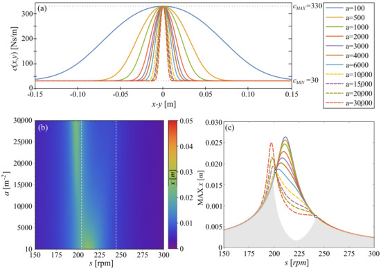
Figure 5.
In panel (a) we show the damping functions (Equation (5)) for selected values of a. In panel (b) we show a two dimensional plot of maximum amplitude of damped system () in two parameters of space: a and s. The last panel (c) shows eleven exemplary FRCs of damped system.
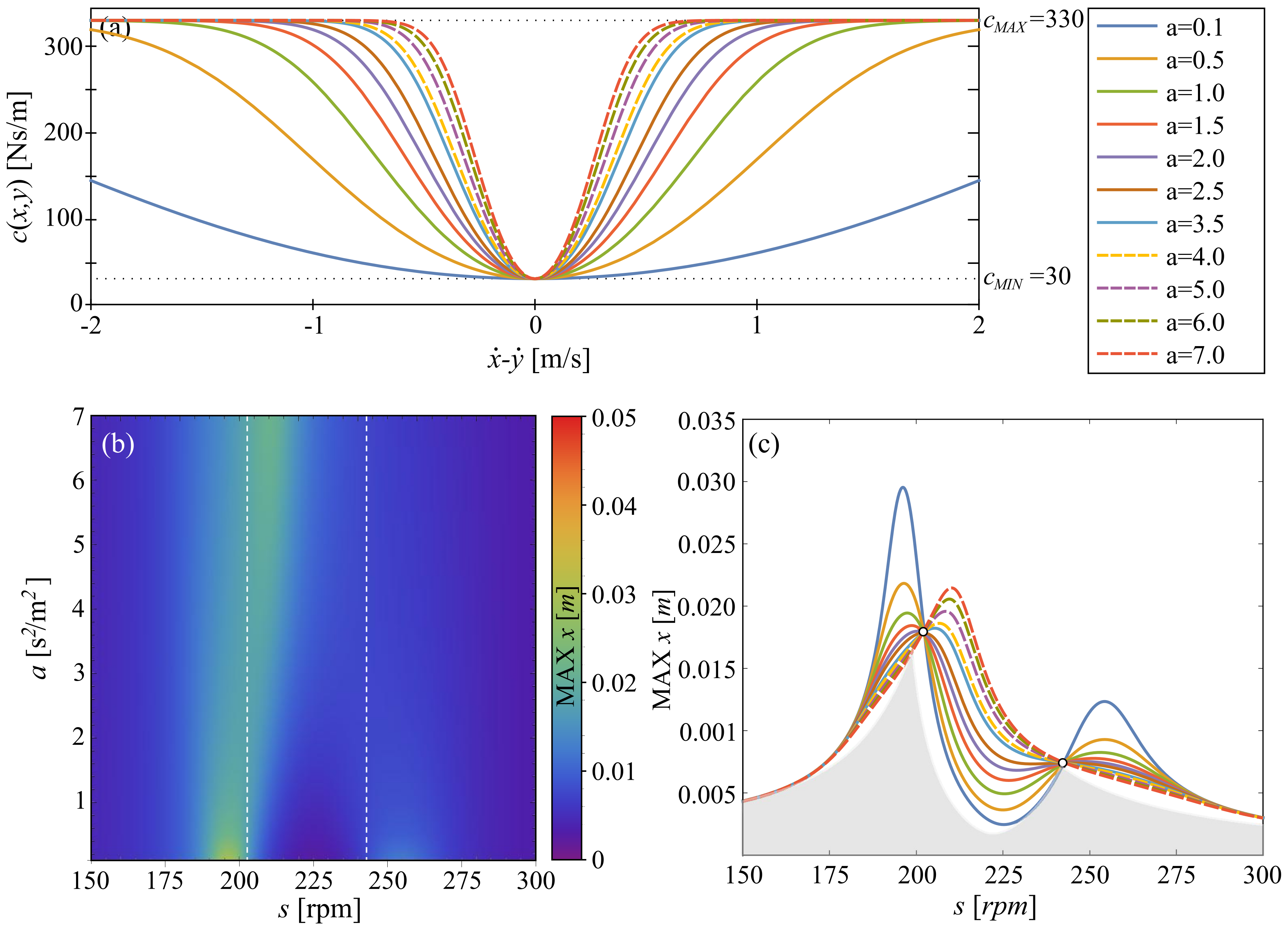
Finally, we analyze strategy 4, which refers to the following function:
where . The exemplary functions are shown in Figure 6a. In this case, as shown in Figure 6b,c, we observe a significantly different scenario than in the previous three cases. For the low value of a (until ) the FRC is continuous, and there are no bifurcations along it. Locations of points P and Q barely change. However, for higher values of a we observe a destabilization of periodic solutions via saddle-node (orange dashed line) and torus (black dashed line) bifurcations. The location of P and Q points can be shifted only by changing the natural frequency of the TMDI or via destabilization of periodic solutions. However, as also for strategy 4, we obtain worse overall damping efficiency than for strategy 0.
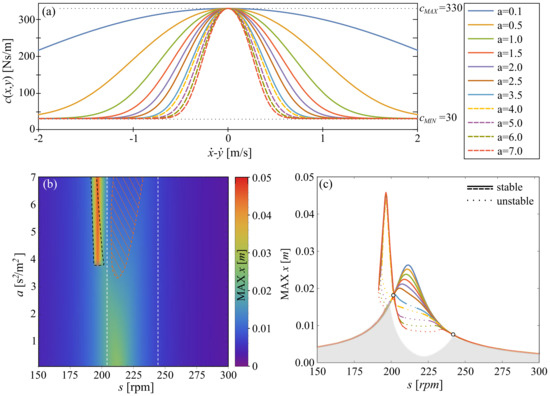
Figure 6.
In panel (a) we show the damping functions (Equation (6)) for selected values of a. In panel (b) we show two dimensional plot of maximum amplitude of damped system () in two parameters of space: a and s. The last panel (c) shows eleven exemplary FRCs of damped system.
With all the first four strategies 1, 2, 3, and 4, we are not able to obtain a better response than for a much simpler strategy 0. The obtained results lead to the conclusion that the usage of non-linear continuous function to change the value of damping coefficient will not bring better results than just setting the proper fixed value basing on the current frequency of excitation. Please note that strategies 1 and 2 were briefly described in our previous paper [33], but to have the lucid presentation of results, we also show them here.
6. Piecewise Damping Functions—Strategies 5, 6, 7, 8
In this section, we analyze control strategies assuming piecewise damping functions; namely, strategies 5, 6, 7, and 8. The damping function depends on the retaliative displacement (strategies 5 and 7) or velocity (strategies 6 and 8) between the main system and the TMDI. For the sake of generality, we include all state variables in the general form of damping function. In each case, we consider the increase or the decrease in damping coefficient and investigate the response for different values of parameter a that describe ranges for c value. The system is no longer smooth. Hence we perform all simulations using direct numerical integration (Runge–Kutta fourth order method).
First, we consider strategy 5 that refers to the following function:
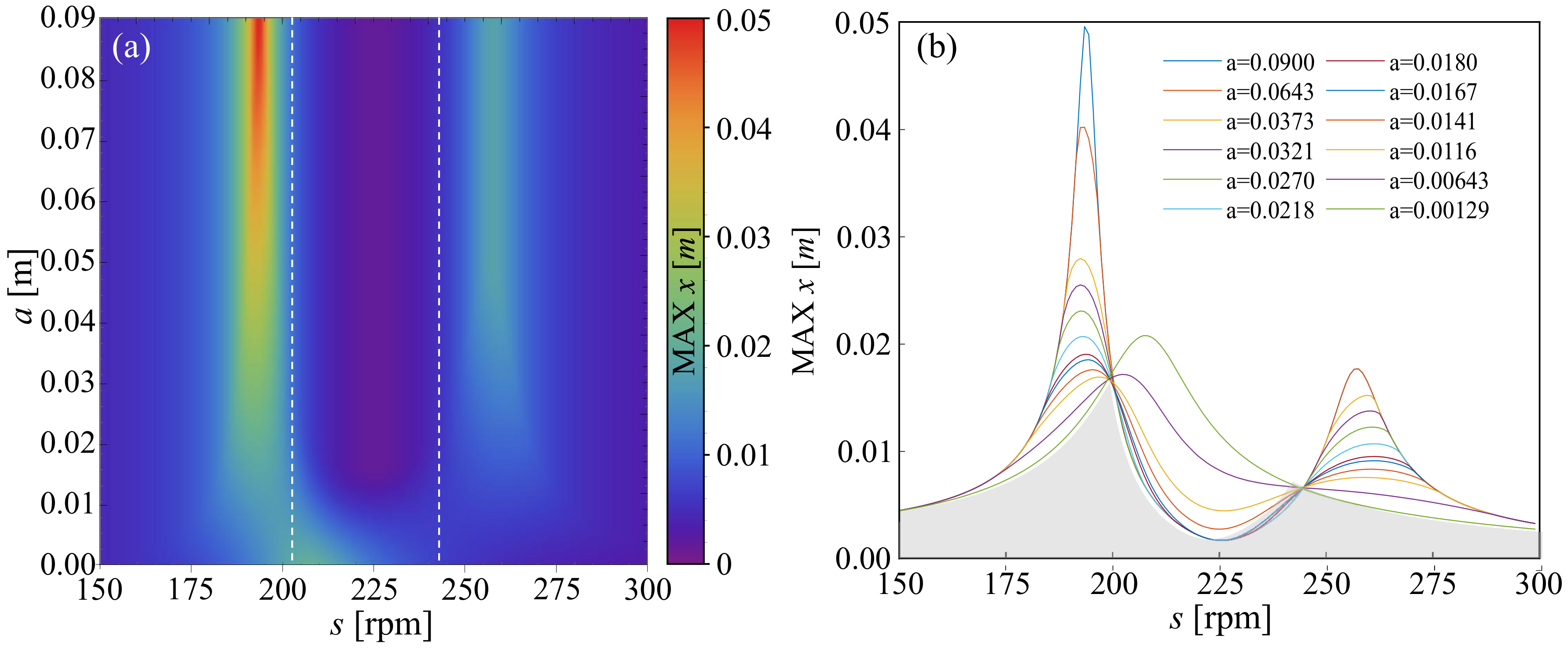
where . The upper value of a corresponds to maximum relative displacement observed in the system for . The results are shown in Figure 7 using the scheme presented in the previous section. In panel (a) we present a two-dimensional color plot of maximum amplitude of the main system as a function of rotational speed s (frequency of excitation) and a parameter of damping function a. White dash lines indicate the location of points P ( [rpm]) and Q ( [rpm]) for the system with linear viscous damping. In Figure 7b, we show twelve exemplary FRCs for equally spaced values of parameter a within the considered range. As it is easy to see, the locations of points P and Q change only slightly when we apply the considered strategy, while the FRCs are significantly different. The non-linear damping function barely decreases the response of the system in the range . Outside range , with the increase in a value, two resonance peaks become more narrow and their maximums increase. With strategy 5, we can slightly increase the damping efficiency of the TMDI when compared to strategy 0, only around point Q. Outside the small range around point Q, the obtained TMD efficiency is no better obtained than with a much simpler strategy 0.

Figure 7.
In panel (a) we show two dimensional plot of maximum amplitude of damped system () in two parameters of space: a and s for damping function given by equation (Equation (7)). Panel (b) shows twelve exemplary FRCs of damped system.
In strategy 6, the value of c depends on the relative velocity between the damped mass and TMDI, following the discontinuous function:
where . The upper value of a corresponds to maximum relative velocity in system with constant linear damping equal to . The results are shown in Figure 8. In panel (a) we can see a maximum amplitude of damped system as a function of a and angular velocity of servomotor . For values of a close to the upper bound, we observe two resonances. Both of them start to reduce gradually with the decrease in a value, which corresponds to the increase in overall damping. When we see a significant change in the character of the response, namely transformation from two resonance peaks to one peak. In panel (b) we see twelve exemplary FRCs where the non-linear character of damping function is clearly visible with the breakdown of FRCs. Using strategy 6 around points P and Q, we can reduce the amplitude of the system below values achievable with strategy 0 (constant value of damping coefficient). However, the reduction occurs for a very narrow range and does not have a significant influence on overall TMDI performance.
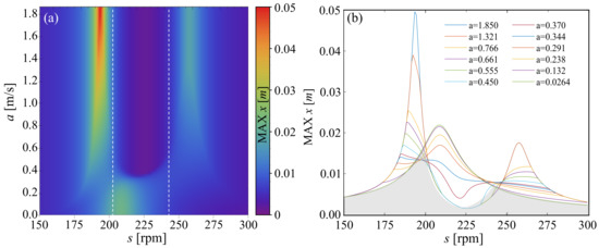
Figure 8.
In panel (a), we show two dimensional plots of maximum amplitude of damped system () in two parameters of space: a and s for damping function given by equation (Equation (8)). Panel (b) shows twelve exemplary FRCs of damped system.
In strategy 7, we consider the following damping function:
where . The upper value of a corresponds to maximum relative displacement in system with constant linear damping equal to . The obtained results are shown in Figure 9a in the same projection as previously. We can see that, until , the system behaves as one DoF system, and all FRCs are nearly indistinguishable, as shown in Figure 9b. The transition in FRC occurs around , and for lower values of a we observe two resonance peaks. With strategy 7, we can reduce the amplitude of the main mass around the point Q when compared to strategy 0, but the amplitude around point P is always bigger, hence by using strategy 7 we are not able to obtain many gains in TMDI efficiency.
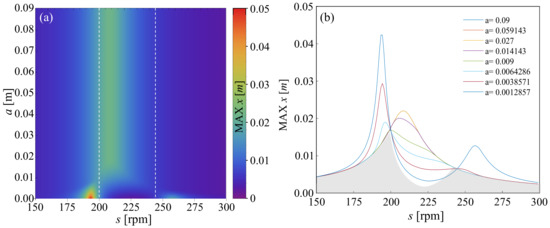
Figure 9.
In panel (a), we show two dimensional plot of maximum amplitude of damped system () in two parameters space: a and s for damping function given by equation (Equation (9)). Panel (b) shows eight exemplary FRCs of damped system
The last considered strategy 8 assumes the following damping function:
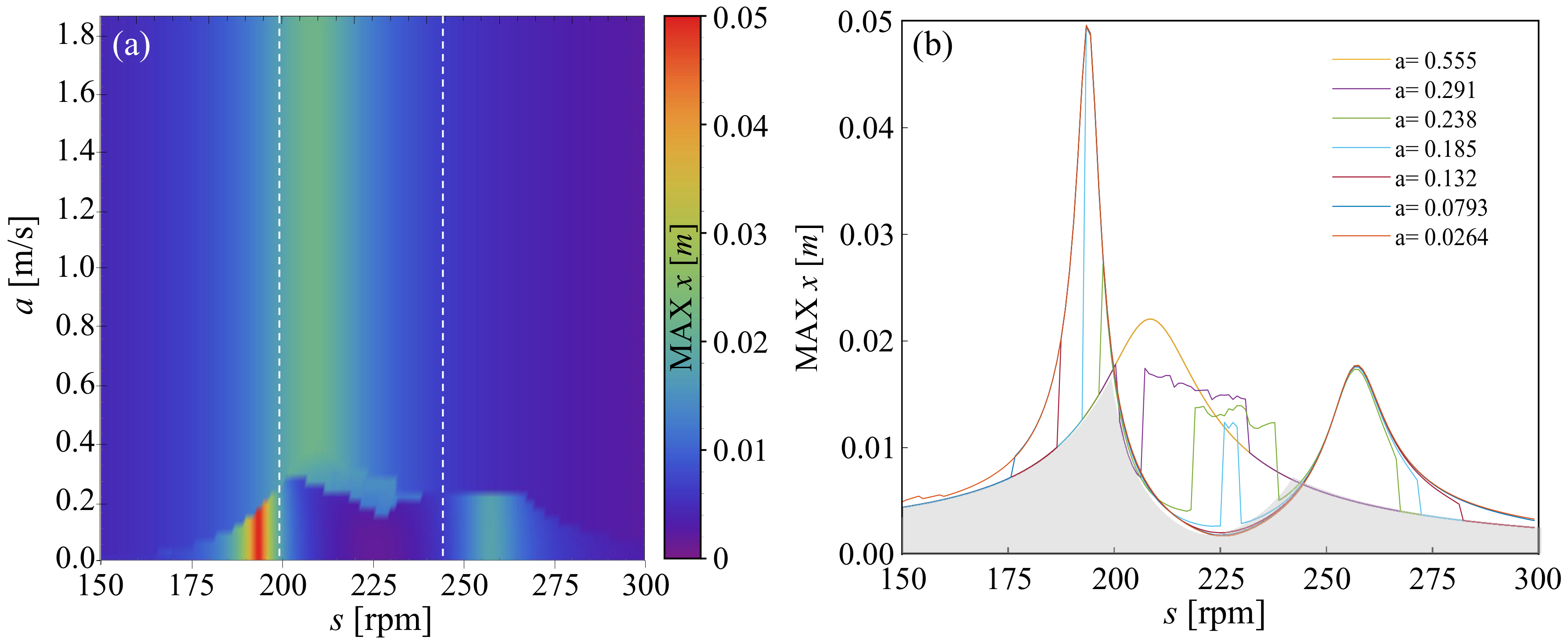
where . The upper value of a corresponds to the maximum relative displacement in system with constant linear damping equals to . As shown in Figure 10a for we see just one resonance peak, and frequency response curves barely change with the increase in a value. Hence, the system behaves like a simple one DoF oscillator. However, for , we see a rapid transition to two resonance response with a narrow area of chaotic behavior. It is clearly visible in Figure 10b, where we show the FRCs for seven selected values of a. With strategy 8, we cannot obtain a gain in the TMDI efficiency when compared to strategy 0. Moreover, we observe sudden changes in system behavior and chaotic solutions, which is highly undesirable.

Figure 10.
In panel (a) we show two dimensional plot of maximum amplitude of damped system () in two parameters of space: a and s for damping function given by equation (Equation (10)). Panel (b) shows seven exemplary FRCs of damped system.
7. Conclusions
In this paper, we describe the non-linear dash-pot’s influence with variable damping coefficient placed between the main mass and the TMDI. We analyze eight different types of damping coefficient control to provide a broad overview of the possible responses. At the beginning of the study, we investigate the response of the system with a linear dash-pot to give a reference. There are two points along the FRC that do not depend on the value damping coefficients, known as points P and Q, and they are also preserved for the non-linear damper. The lowest amplitude of the system is reached when the damping coefficient changes from its minimum to the maximum value between points P and Q. In such a case, the main system always follows a solution with minimum amplitude. Such control is equivalent to bang–bang control. In the main part of the study, we investigate how, by using the non-linear dash-pot and the inerter, we can further decrease the maximum amplitude of the damped body. The analysis proves that suspicion of the stationary character of points P and Q is true even when the non-linear damper is used. However, we find ranges where one can observe the decrease in the amplitude of the main system when compared to bang–bang control. By changing the damping coefficient, one can achieve different responses of the main system and control its behavior in the desired way. Based on the presented comprehensive study, one can easily find the control to achieve the expected dynamics.
Author Contributions
Conceptualization, P.P. and P.B.; methodology: P.P. and P.B.; formal analysis, M.L. and P.B.; investigation M.L. and P.B.; validation, P.P.; software, P.B. and M.L.; writing—original draft preparation, M.L. and P.B.; writing—review and editing, P.P.; funding acquisition, P.P. All authors have read and agreed to the published version of the manuscript.
Funding
This work has been supported by National Science Centre, Poland—Project No. 2015/17/B/ST8/03325.
Conflicts of Interest
The authors declare that they have no conflict of interest.
References
- Frahm, H. Device for Damping Vibrations of Bodies. U.S. Patent No. 989958A, 30 October 1909. [Google Scholar]
- Den Hartog, J.P. Mechanical Vibrations; McGraw-Hill: New York, NY, USA, 1934. [Google Scholar]
- Habib, G.; Kádár, F.; Papp, B. Impulsive vibration mitigation through a nonlinear tuned vibration absorber. Nonlinear Dyn. 2019, 98, 2115–2130. [Google Scholar] [CrossRef]
- Iurasov, V.; Mattei, P.-O. Bistable nonlinear damper based on a buckled beam configuration. Nonlinear Dyn. 2019, 99, 1801–1822. [Google Scholar] [CrossRef]
- Dekemele, K.; Van Torre, P.; Loccufier, M. Performance and tuning of a chaotic bi-stable NES to mitigate transient vibrations. Nonlinear Dyn. 2019, 98, 1831–1851. [Google Scholar] [CrossRef]
- Zhang, Z.; Nielsen, S.R.; Blaabjerg, F.; Zhou, D. Dynamics and control of lateral tower vibrations in offshore wind turbines by means of active generator torque. Energies 2014, 7, 7746–7772. [Google Scholar] [CrossRef]
- Tophøj, L.; Grathwol, N.; Hansen, S.O. Effective Mass of Tuned Mass Dampers. Vibration 2018, 1, 192–206. [Google Scholar] [CrossRef]
- Cho, S.G.; Chang, S.; Sung, D. Application of Tuned Mass Damper to Mitigation of the Seismic Responses of Electrical Equipment in Nuclear Power Plants. Energies 2020, 13, 427. [Google Scholar] [CrossRef]
- Kwag, S.; Kwak, J.; Lee, H.; Oh, J.; Koo, G.-H. Enhancement in the Seismic Performance of a Nuclear Piping System using Multiple Tuned Mass Dampers. Energies 2019, 12, 2077. [Google Scholar] [CrossRef]
- Lian, J.; Zhao, Y.; Lian, C.; Wang, H.; Dong, X.; Jiang, Q.; Zhou, H.; Jiang, J. Application of an Eddy Current-Tuned Mass Damper to Vibration Mitigation of Offshore Wind Turbines. Energies 2018, 11, 3319. [Google Scholar] [CrossRef]
- Wang, F.-C.; Smith, M.C. Performance benefits in passive vehicle suspensions employing inerters. Proc. IEEE Conf. Decis. Control 2004, 3, 2258–2263. [Google Scholar]
- Papageorgiou, C.; Houghton, N.E.; Smith, M.C. Experimental testing and analysis of inerter devices. J. Dyn. Syst. Meas. Control 2009, 131, 011001–011011. [Google Scholar] [CrossRef]
- Smith, M.; Swift, S. Design of passive vehicle suspensions for maximal least damping ratio. Veh. Syst. Dyn. 2006, 54, 568–584. [Google Scholar] [CrossRef]
- Madhamshetty, K.; Manimala, J.M. Low-Rate Characterization of a Mechanical Inerter. Machines 2018, 6, 32. [Google Scholar] [CrossRef]
- Smith, M. Synthesis of mechanical networks: The inerter. IEEE Trans. Autom. Control 2002, 47, 1648–1662. [Google Scholar] [CrossRef]
- Chen, M.; Papageorgiou, C.; Scheibe, F.; Wang, F.-C.; Smith, M. The missing mechanical circuit element. Circ. Syst. Mag. IEEE 2009, 9, 10–26. [Google Scholar] [CrossRef]
- Wang, F.-C.; Liao, M.-K. The lateral stability of train suspension systems employing inerters. Veh. Syst. Dyn. 2010, 48, 619–643. [Google Scholar] [CrossRef]
- Wang, F.-C.; Hsieh, M.-R.; Chen, H.-J. Stability and performance analysis of a full-train system with inerters. Veh. Syst. Dyn. 2012, 50, 545–571. [Google Scholar] [CrossRef]
- Borowski, J.; Stetter, R.; Rudolph, S. Design, Dimensioning and Simulation of Inerters for the Reduction of Vehicle Wheel Vibrations—Case Studies. Vehicles 2020, 2, 424–437. [Google Scholar] [CrossRef]
- Faraj, R.; Holnicki-Szulc, J.; Knap, L.; Senko, J. Adaptive inertial shock-absorber. Smart Mater. Struct. 2016, 25, 035031. [Google Scholar] [CrossRef]
- Takewaki, I.; Murakami, S.; Yoshitomi, S.; Tsuji, M. Fundamental mechanism of earthquake response reduction in building structures with inertial dampers. Struct. Control Health Monit. 2012, 19, 590–608. [Google Scholar] [CrossRef]
- Chen, Y.-C.; Tu, J.-Y.; Wang, F.-C. Earthquake vibration control for buildings with inerter networks. In Proceedings of the Control Conference (ECC) (2015 European), Linz, Austria, 15–17 July 2015; pp. 3137–3142. [Google Scholar]
- De Domenico, D.; Ricciardi, G. An enhanced base isolation system equipped with optimal tuned mass damper inerter (tmdi). Earthq. Eng. Struct. Dyn. 2018, 47, 1169–1192. [Google Scholar] [CrossRef]
- Giaralis, A.; Taflanidis, A. Optimal tuned mass-damper-inerter (TMDI) design for seismically excited mdof structures with model uncertainties based on reliability criteria. Struct. Control. Health Monit. 2018, 25, e2082. [Google Scholar] [CrossRef]
- Yang, J.; Jiang, J.Z.; Neild, S.A. Dynamic analysis and performance evaluation of nonlinear inerter-based vibration isolators. Nonlinear Dyn. 2020, 99, 1823–1839. [Google Scholar] [CrossRef]
- Zhang, Z.; Zhang, Y.-W.; Ding, H. Vibration control combining nonlinear isolation and nonlinear absorption. Nonlinear Dyn. 2020, 100, 1–19. [Google Scholar] [CrossRef]
- De Haro Moraes, M.; Silveira, F.M.; Gonçalves, P.J.P. On the dynamics of a vibration isolator with geometrically nonlinear inerter. Nonlinear Dyn. 2018, 93, 1325–1340. [Google Scholar] [CrossRef]
- Xie, L.; Ban, X.; Xue, S.; Ikago, K.; Kang, J.; Tang, H. Theoretical Study on a Cable-Bracing Inerter System for Seismic Mitigation. Appl. Sci. 2019, 9, 4096. [Google Scholar] [CrossRef]
- Lazarek, M.; Brzeski, P.; Perlikowski, P. Novel type of tuned mass damper with inerter which enables changes of inertance. J. Sound Vib. 2015, 349, 56–66. [Google Scholar]
- Lazarek, M.; Brzeski, P.; Perlikowski, P. Experimental study of the novel tuned mass damper with inerter which enables changes of inertance. J. Sound Vib. 2017, 404, 47–57. [Google Scholar]
- Lazarek, M.; Brzeski, P.; Perlikowski, P. Design and identification of parameters of tuned mass damper with inerter which enables changes of inertance. Mech. Mach. Theory 2018, 119, 161–173. [Google Scholar] [CrossRef]
- Lazarek, M.; Brzeski, P.; Perlikowski, P. Design and modeling of the cvt for adjustable inerter. J. Frankl. Inst. 2018, 365, 7611–7625. [Google Scholar] [CrossRef]
- Lazarek, M.; Brzeski, P.; Perlikowski, P. Influence of dash-pot with controllable damping coefficient on damping efficiency of TMDI. MATEC Web Conf. 2018, 148, 02001. [Google Scholar] [CrossRef][Green Version]
- De Domenico, D.; Deastra, P.; Ricciardi, G.; Sims, N.D.; Wagg, D.J. Novel fluid inerter based tuned mass dampers for optimised structural control of base-isolated buildings. J. Frankl. Inst. 2019, 356, 7626–7649. [Google Scholar] [CrossRef]
- Nakai, T.; Kurino, H.; Yaguchi, T.; Kano, N. Control effect of large tuned mass damper used for seismic retrofitting of existing high-rise building. Jpn. Archit. Rev. 2019, 2, 269–286. [Google Scholar] [CrossRef]
- Shi, W.; Wang, L.; Lu, Z.; Gao, H. Study on adaptive-passive and semi-active eddy current tuned mass damper with variable damping. Sustainability 2018, 10, 99. [Google Scholar] [CrossRef]
- Zhao, Z.; Dai, K.; Lalonde, E.R.; Meng, J.; Li, B.; Ding, Z.; Bitsuamlak, G. Studies on application of scissor-jack braced viscous damper system in wind turbines under seismic and wind loads. Eng. Struct. 2019, 196, 109294. [Google Scholar] [CrossRef]
Publisher’s Note: MDPI stays neutral with regard to jurisdictional claims in published maps and institutional affiliations. |
© 2020 by the authors. Licensee MDPI, Basel, Switzerland. This article is an open access article distributed under the terms and conditions of the Creative Commons Attribution (CC BY) license (http://creativecommons.org/licenses/by/4.0/).

