Virtual State Feedback Reference Tuning and Value Iteration Reinforcement Learning for Unknown Observable Systems Control

Abstract

In this paper, a novel Virtual State-feedback Reference Feedback Tuning (VSFRT) and Approximate Iterative Value Iteration Reinforcement Learning (AI-VIRL) are applied for learning linear reference model output (LRMO) tracking control of observable systems with unknown dynamics. For the observable system, a new state representation in terms of input/output (IO) data is derived. Consequently, the Virtual State Feedback Tuning (VRFT)-based solution is redefined to accommodate virtual state feedback control, leading to an original stability-certified Virtual State-Feedback Reference Tuning (VSFRT) concept. Both VSFRT and AI-VIRL use neural networks controllers. We find that AI-VIRL is significantly more computationally demanding and more sensitive to the exploration settings, while leading to inferior LRMO tracking performance when compared to VSFRT. It is not helped either by transfer learning the VSFRT control as initialization for AI-VIRL. State dimensionality reduction using machine learning techniques such as principal component analysis and autoencoders does not improve on the best learned tracking performance however it trades off the learning complexity. Surprisingly, unlike AI-VIRL, the VSFRT control is one-shot (non-iterative) and learns stabilizing controllers even in poorly, open-loop explored environments, proving to be superior in learning LRMO tracking control. Validation on two nonlinear coupled multivariable complex systems serves as a comprehensive case study.

1. Introduction

Learning control from input/output (IO) system data is a current significant research area. The idea stems from the data-driven control research, where it is strongly believed that the gap between an identified system model and the true system is an important factor leading to control performance degradation.

Value Iteration (VI) is one popular approximate dynamic programming [1,2,3,4,5,6,7] and reinforcement learning algorithm [8,9,10,11,12,13], together with Policy Iteration. VI Reinforcement Learning (VIRL) algorithm comes in many implementation flavors, online or offline, off-policy or on-policy, batch-wise or adaptive-wise, with known or unknown system dynamics. In this work, the class of offline off-policy VIRL for unknown dynamical systems is adopted, based on neural networks (NNs) function approximators, hence it will be coined as Approximate Iterative VIRL (AI-VIRL). For this model-free offline off-policy learning variant, a database of transition samples (or experiences) is required to learn the optimal control. Most practical implementations are of the actor-critic type where function approximators (most often neural networks (NNs)) are used to approximate the cost function and the controller, respectively.

One of the crucial aspects of AI-VIRL convergence is appropriate exploration, translated to visiting as many state-actions combinations as possible while uniformly covering the state-action domains. The exploration aspect is especially problematic with general nonlinear systems whereas for linear ones, linearly parameterized function approximators for the cost function and for the controller, relieve to some extent this issue, owing to their better generalization capacity. Good exploration is not easily achieved in uncontrolled environments, and usually, pre-existing stabilizing controllers can increase the exploration quality significantly. An additional reason for using pre-stabilizing controller is that, in mechatronics systems, uncontrolled environment commonly implies instability, under which dangerous conditions could lead to physical damage. This is different from the virtual environments specific, e.g., to video games [14] (or even simulated mechatronics systems), where instability leads to an episode (or simulation) termination but physical damage is not a threat.

Another issue with reinforcement learning algorithms such as AI-VIRL, is the state representation. Most often, in the case of unknown systems, the measured data from the system cannot be assumed to fully capture the system state, leading to the partial observability learning issues associated with the reinforcement learning algorithms [15,16,17,18]. Therefore, new state representations are needed to ensure that learning takes place in a fully observable environment. A new state representation is proposed in this work based on the assumption that the controlled system is observable. Therefore, a virtual state built from present and past IO samples is introduced as an alias for the true state. The new virtual state-space representation is a fully observable system which allows controlling the original underlying system.

A similar approach to AI-VIRL for learning optimal control in offline off-policy mode is Virtual Reference Feedback Tuning (VRFT) [19,20,21,22,23,24,25]. It also relies on a database of (usually IO) samples collected from the system in a dedicated experimental interaction step. Traditionally, VRFT was proposed for output feedback error IO controllers and was not sufficiently exploited for state-feedback control yet. Certainly not for the virtual state-feedback control required by observable systems for which direct state measurement is impossible. One contribution of this work is to propose for the first time such a model-free framework called Virtual State-Feedback Reference Tuning (VSFRT), which learns control based on the feedback provided by the virtual state representation.

VSFRT also requires exploration of the controlled system dynamics by using persistently excited input signals, in order to visit many IO (or input-state-output) combinations. Principally, it turns the system identification problem into a direct controller identification problem. This paradigm shift can be thought of as a typical supervised machine learning problem, especially since VRFT has been used before with NN controllers [24,25,26,27]. To date, VRFT has been applied mainly for output-feedback error-based IO controllers with few reported results with state-feedback control [26,27] but not with feedback control based on a virtual state constructed from IO data.

Both AI-VIRL and VRFT lend themselves to the reference model output tracking problem framework. It is therefore of interest to compare their learning capacity in terms of resources needed, achievable tracking performance, sensitivity to the exploration issue and type of approximators being used. In particular, the linear reference model output (LRMO) tracking control setting is advantageous, ensuring indirect state-feedback linearization of control systems. Such linearity property of control systems is critical for higher-level learning paradigms such as Iterative Learning Control [28,29,30,31,32,33,34] and primitive-based learning [34,35,36,37,38,39,40], as representative hierarchical learning control paradigms [41,42,43,44].

The contributions of this work are:

• A new state representation for systems with unknown dynamics. A virtual state is constructed from historical input/output data samples, under observability assumptions.
• An original Virtual State Feedback Reference Tuning (VSFRT) neural controller tuning based on the new state representation. Stability certification is analyzed.
• Performance comparison of VSFRT and AI-VIRL data-driven neural controllers for LRMO tracking.
• Analysis of the transfer learning suitability for the VSFRT controller to provide initial admissible controllers for the iterative AI-VIRL process.
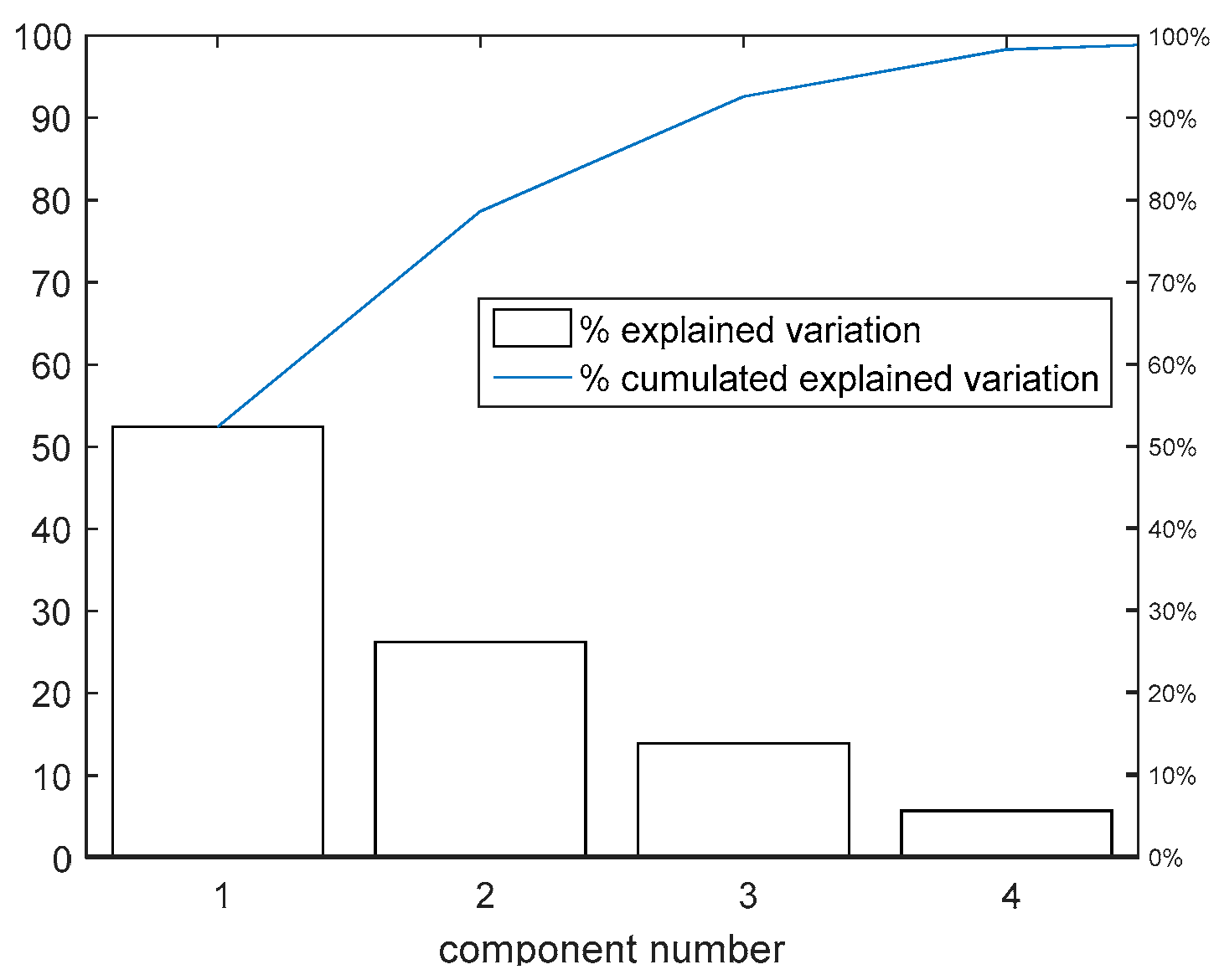
• Analyze the impact of the state representation dimensionality reduction upon the learning performance using unsupervised machine learning tools such as principal component analysis (PCA) and autoencoders (AE).

Section 2 introduces the LRMO tracking problem formulation while Section 3 proposes the VSFRT and the AI-VIRL solution concepts. The two comprehensive validation case studies of Section 4 and Section 5, respectively, validate this work’s objectives. Conclusions are presented in the last Section 6.

2. The LRMO Tracking Problem

Let the dynamical discrete-time system be described by the state-space plus output model equation

$$\{\begin{array}{l}{s}_{k+1}=f(s_k,u_k),\\ y_k=g(s_k),\end{array}$$

(1)

where $s_k={[s_{k,1}\dots s_{k,n}]}^T$ is the un-measurable state, the control input is $u_k={[u_{k,1},\dots ,u_{k,m_u}]}^T$ while $y_k={[y_{k,1},\dots ,y_{k,p}]}^T$ is the sensed output. The dynamics f, g of (1) are unknown but considered continuously differentiable (CD) maps. Additional assumption about (1) require that it is IO observable and controllable. The IO observability implies that, as in the case of the more well-known linear systems, the state can be fully recovered from system present and past IO samples. Given the observable system (1), IO samples $u_k,y_k$ are employed to form a virtual state-space model having $u_k$ as input and $y_k$ as output (similarly to (1)), with a different state vector, according to [45]. This resulted virtual state-space model is:

$$\begin{array}{l}{v}_{k+1}=F(v_k,u_k),\\ y_k=v_{k,1},\end{array}$$

(2)

defined in terms of the virtual state vector $v_k={[Y_{\overline{k,k-\tau }}^T,U_{\overline{k-1,k-\tau }}^T]}^T\stackrel{\mathsf{\Delta }}{=}[v_{k,1},v_{k,2},\dots v_{k,2\tau +1}]\in {\Re }^{p(\tau +1)+m_u\tau }$, with $Y_{\overline{k,k-\tau }}={[y_k^T\dots y_{k-\tau }^T]}^T\stackrel{\mathsf{\Delta }}{=}{[v_{k,1}^T\dots v_{k,\tau +1}^T]}^T$, $U_{\overline{k-1,k-\tau }}={[u_{k-1}^T\dots u_{k-\tau }^T]}^T\stackrel{\mathsf{\Delta }}{=}$${[v_{k,\tau +2}^T\dots v_{k,2\tau +1}^T]}^T$ (upper T means vector/matrix transposition). Model (2) has partially known dynamics (the unknown part stems from unknown dynamics of (1)) and it is fully state observable [45]. Such transformations are well-known for linear systems. Here, $\tau$ is correlated with the observability index and should be chosen empirically since it cannot be established analytically due to partially unknown dynamics. It should be selected as large as possible, accounting for the fact that for a value larger than the true observability index, there is no more information gain in explaining the true state $s_k$ through $v_k$ [45]. The observability index is well-known in linear systems theory (please consult Appendix A). Its minimal value K for which $\tau \ge K$, ensures that the observability matrix has its full column rank equal to the state dimension $n$. Meaning that the state is fully observable from a number of at least K past input samples and at least K past output samples. In the light of the above remark, we define the unknown observability index of the nonlinear system (1) as the minimal value K for which any $\tau \ge K$ ensures that $s_k$ is observable from $Y_{\overline{k,k-\tau }}$, $U_{\overline{k-1,k-\tau }}$. Transformations such as (2) can easily accommodate time delays in the input/state of (1) by properly introducing supplementary states. Such operations preserve the full observability of (2) [45].

IO controlling (2) is the same with IO controlling (1), since they have the same input and output. While any potential state-feedback control mapping the state to the control input, would differ for (1) and (2) since $s_k\in {\Re }^n$ and $v_k\in {\Re }^{p(\tau +1)+m_u\tau }$. The control objective is aimed at shaping the IO behavior of (1) by indirectly controlling the IO behavior of (2) through state-feedback. This is achieved by the reference model output tracking framework, presented next.

A strictly causal linear reference model (LRM) is:

$$\{\begin{array}{l}{s}_{k+1}^m=G{s}_k^m+H{r}_k,\\ y_k^m=L{s}_k^m,\end{array}$$

(3)

where the LRM state is $s_k^m={[s_{k,1}^m,\dots ,s_{k,n_m}^m]}^T$, the LRM input $r_k={[r_{k,1},\dots ,r_{k,p}]}^T$ will be reference input to the control system and the LRM output is $y_k^m={[y_{k,1}^m,\dots ,y_{k,p}^m]}^T$. The LRM dynamics are known and characterized by the matrices $G,H,L$. Its linear pulse transfer matrix IO dependence can be established as $y_k^m=T_{LRM}(q)r_k$, where “q” is the pulse transfer time-based operator, analogous to the “z” operator.

The LRMO tracking goal is to search for the control input which causes the system’s (1) output $y_k$ to track the output $y_k^m$ of the LRM (3), given any reference input $r_k$. This objective is captured as an optimal control problem searching for the optimal input satisfying

$$\begin{array}{l}{u}_k^{*}=\arg \underset{u_k}{\min }{V}_{LRMO}^{\infty },V_{LRMO}^{\infty }={\displaystyle \sum _{k=0}^{\infty }{\Vert y_k(u_k)-y_k^m\Vert }_2^2},\\ s.t.(1),(3),\end{array}$$

(4)

where the dependence of $y_k$ on $u_k$ is suggested. In the expression above, ${\Vert •\Vert }_2$ measures the L² distance over vectors. It is assumed that a solution $u_k^{*}$ for (4) exists. The above control problem is a form of imitation learning where the LRM is the “expert” (or teacher or supervisor) and the system (1) is a learner which must mimic the LRM’s IO behavior. For the given problem, dynamics of (3) must be designed beforehand, however they may be unknown to the learner system (1).

In the subsequent section, the problem (4) is solved by learning two state-feedback closed-loop control solutions for the system (2). The implication is straightforward. If a state-feedback controller of the form $u_k^{}=C(v_k)$ is learned to control (2), then this control action can be set as the actual control input for the system (1), based on the feedback $v_k$ built from present and past IO samples $u_k,y_k$ of the system (1). Hence, learning control for (2) by solving (4) is the same with solving (4) for the underlying system (1). Notice the recurrence in $u_k^{}=C(v_k)$ since $v_k$ includes $u_{k-1},\dots ,u_{k-\tau }$.

Several observations concerning the LRM selection are mentioned. According to the classical control rules in model reference control [46], the LRM dynamics must be correlated with the bandwidth of the system (1). The time-delay of (1) and its possible non-minimum-phase (NMP) character must be accounted for inside the LRM as they should not be compensated. These knowledge requirements are satisfiable based on working experience with the system or from technical datasheets. However, they do not interfere with the “unknown dynamics” assumption. Since the virtual state-feedback control design is attempted based on the VSFRT principle, it is known from classical VRFT control that the NMP property of (1) requires special care, therefore for simplification, it will be assumed that (1) is minimum-phase. IO data collection necessary for both the VSFRT and the AI-VIRL designs require that (1) is either open-loop stable or stabilized in closed-loop. It will be assumed further that (1) is open-loop stable, although closed-loop stabilization for IO samples collections can (and will also) be employed for reducing collection phase duration and to enhance exploration.

The following section proposes and details the VSFRT and AI-VIRL for learning optimal control in (4), in virtual state feedback-based closed-form solutions.

3. LRM Output Tracking Problem Solution

3.1. Recapitulating VRFT for Error-Feedback IO Control

In the well-known VRFT for error-feedback control defined for linear mono-variable unknown systems [19], a database of IO samples is considered available after being collected from the base system (1), let this database be called $DB=\{(u_k,y_k)\},k=\overline{0,N-1}$. Either open- or closed-loop could be considered for IO samples collection. Based on the VRFT principle, it is assumed that $y_k$ is also the output of the given LRM conveyed by $T_{LRM}(q)$. One can offline calculate in a noncausal fashion the virtual reference ${\tilde{r}}_k=T_{LRM}^{-1}(q)y_k$ which set as input to $T_{LRM}^{}(q)$ would render $y_k$ at its output. The tilde means offline calculation. A virtual feedback error is next defined as ${\tilde{e}}_k={\tilde{r}}_k-y_k$. Selecting some prior linear controller transfer function structure $C({\tilde{e}}_k,\vartheta )$ ($\vartheta$-the parameter vector) as a function of the virtual feedback error, the controller identification problem is defined as the minimization over $\vartheta$ of the cost $V_{VR}^N(\vartheta )=\frac{1}{N}{\displaystyle \sum _{k=0}^{N-1}{\Vert u_k^{}-C({\tilde{e}}_k^{},\vartheta )\Vert }_2^2}$. Meaning that the controller $C({\tilde{e}}_k,\vartheta )$ outputs $u_k$ when driven by ${\tilde{e}}_k$. This conceptually implies that the control system having the loop closed by $C({\tilde{e}}_k,\vartheta )$, produces the signals $u_k$ and $y_k$ when driven by ${\tilde{r}}_k$. This would eventually match the closed-loop with the LRM. The VRFT circumvents direct controlled system identification, hence it is model-free.

The work [19] analyzed approximate theoretical equivalence between $V_{VR}^N(\vartheta )$ and the LRM cost $V_{LRMO}^{\infty }={\displaystyle \sum _{k=0}^{\infty }{\Vert y_k(u_k)-y_k^m\Vert }_2^2}$ from (4). A linear prefilter called “the L-filter” (sometimes denoted with M) with pulse transfer function L(q), was used to enhance this equivalence by replacing $u_k,{\tilde{e}}_k$ in $V_{VR}^N(\vartheta )$ with their filtered variants $u_k^L=L(q)u_k,{\tilde{e}}_k^L=L(q){\tilde{e}}_k$. The VRFT extension to the multi-variable case was studied in [20] while its extension to nonlinear system and nonlinear controller case has been afterwards exploited in works like [23,24,25,26,27], where the L-filter was dropped when richly parameterized controllers were used (e.g., NNs).

3.2. VSFRT—The Virtual State Feedback-Based VRFT Solution for the LRM Output Tracking

Following the rationale behind the classical model-free VRFT, a database of IO samples is considered available after being collected from the base system (1), let it be denoted as $DB=\{(u_k,y_k)\},k=\overline{0,N-1}$. It is irrelevant for the following discussion if the samples were collected in open- or closed-loop. An input-state-output database is constructed as $\{(u_k,{\tilde{v}}_k,y_k)\}$ where ${\tilde{v}}_k$ is constructed from the historical data $u_k,y_k$. Based on the VRFT principle, it is assumed that $y_k$ is also the output of the given LRM (characterized by $T_{LRM}(q)$). A non-causal filtering then allows for virtual reference calculation as in ${\tilde{r}}_k=T_{LRM}^{-1}(q)y_k$. Similar to VRFT applied for error-feedback IO control, now a virtual state-feedback reference feedback tuning (VSFRT) controller is searched for. This controller denoted C should make the LRM’s output to be tracked by the system (2)’s output and it is identified to minimize the cost

$$V_{VR}^N(\vartheta )=\frac{1}{N}{\displaystyle \sum _{k=0}^{N-1}{\Vert u_k^{}-C({\tilde{s}}_k^{ex-},\vartheta )\Vert }_2^2}$$

(5)

with ${\tilde{s}}_k^{ex-}=[{({\tilde{v}}_k)}^T{({\tilde{r}}_k)}^T{]}^T$ being an extended state regressor vector constructed from the virtual state ${\tilde{v}}_k$ of (2) and with a controller parameter vector $\vartheta$.

A VSFRT controller rendering $V_{VR}^N(\vartheta )=0$ should lead to $V_{LRMO}^{\infty }\to 0$. It is the VRFT principle which establishes the equivalence between $V_{VR}^N(\vartheta )$ and $V_{LRMO}^{\infty }(\vartheta )$, being supported in practice by using richly parameterized controllers (such as NNs [25]), coupled with a wise selection of the LRM dynamics. A controller NN called C-NN will be employed in this framework, with $\vartheta$ capturing the NN trainable weights. It is straightforward to regard $V_{VR}^N(\vartheta )$ as the mean sum of squared errors (MSSE) criterion for training the C-NN, with input pattern $\left\{{\tilde{s}}_k^{ex-}\right\}$ and with output pattern $\left\{u_k^{}\right\}$.

The model-free VSFRT algorithm is presented below.

• The IO database $DB=\{(u_k,y_k)\},k=\overline{0,N-1}$ is first collected, then ${\tilde{v}}_k$ is built. Both ${\tilde{r}}_k$ and ${\tilde{s}}_k^{ex-}$ are computed.
• A C-NN is parameterized by properly selecting a NN architecture type together with its training details. $MaxTrain$ called the maximum number of training times is set along with the index j = 1 counting the number of trainings.
• The NN weights vector $\vartheta$ is initialized (e.g., randomly).
• The C-NN is trained with input patterns $in=\left\{{\tilde{s}}_k^{ex-}\right\}$ and output patterns $t=\left\{u_k^{}\right\}$. This is equivalent to minimizing (5) w.r.t. $\vartheta$.
• If $j<MaxTrain$, set $j=j+1$ and repeat from the 3^rd Step, otherwise finish the algorithm.

The above algorithm produces several trained neural controllers C-NN with parameter $\vartheta$, i.e $C({\tilde{s}}_k^{ex-},\vartheta )$. The best one is selected based on some predefined criterion (minimal value of $V_{VR}^N(\vartheta )$ or minimal value of some tracking performance on a given test scenario). Stability of the closed-loop with the VSFRT C-NN is asserted, with some assumptions following next [47]:

A1. The system (2) supports the equivalent IO description $y_k=T(y_{k-1},\dots ,y_{k-ny},u_{k-1},\dots ,u_{k-nu}),$ with $ny$, $nu$ unknown system orders and the nonlinear map $T$ is invertible with respect to $u$: For a given $y_k$, the input $u_k$ is computable as $u_{k-1}=T^{-1}(y_k)$ (the “k−1” subscript in u vs. the “k” subscript in y formally suggest strictly causal system). Additionally, LRM (3) supports the IO recurrence $y_k^m=T_{LRM}(y_{k-1}^m,\dots ,y_{k-nym}^m,r_{k-1},\dots ,r_{k-nr})$ with known orders $nym$, $nr$ and $T_{LRM}$ is a linear invertible map with stable inverse, allowing to find $r_{k-1}=T_{LRM}^{-1}(y_k^m)$.

A2. The system (2) and the LRM (3) are formally representable as $y_k=M(v_k,u_{k-1})$ and $y_k^m=M^m(s_k^m,r_{k-1}^{})$, to simultaneously convey the IO and the input-state-output dependence in a single compact form, under the mappings $M,M^m$. With no generality loss, the above representation indicates the relative degree one between input and output. Let us assume the map $M$ is invertible, with $v_k^{},u_{k-1}^{}$ computable from $y_k^{}$ as $v_k^{}={(M_v^{})}^{-1}(y_k^{})$, $u_{k-1}^{}={(M_u^{})}^{-1}(y_k^{})$. Also assume that $M^m$ is a CD invertible map such that $s_k^m,r_{k-1}^{}$ are computable from $y_k^m$ as $s_k^m={(M_s^m)}^{-1}(y_k^m),r_{k-1}^{}={(M_r^m)}^{-1}(y_k^m)$ and that there are constants ${\kappa }_{Mx}^m>0,{\kappa }_{Mr}^m>0$ fulfilling $\Vert \frac{\partial M^m(s_k^m,r_{k-1})}{\partial s_k^m}\Vert <{\kappa }_{Mx}^m$ and $\Vert \frac{\partial M^m(s_k^m,r_{k-1})}{\partial r_{k-1}}\Vert <{\kappa }_{Mr}^m$, where $\Vert •\Vert$ is an appropriate matrix norm induced by the L² vector norm. The model inversion assumptions are natural for state-space systems (2) and (3) being characterized by IO models. Practically, the idea behind $v_k^{}={(M_v^{})}^{-1}(y_k^{})$ is as follows: For certain $y_k$ in (2), one can calculate $u_{k-1}=T^{-1}(y_k)$, then generate $v_{k+1}=F(v_k,u_k)$ based on (2). The above inequalities with upper bounds on the maps’ partial derivatives are reasonable and commonly used in control. Moreover, let $M,{(M_v)}^{-1}$ be continuously differentiable (CD) and of bounded derivative to satisfy

$$\begin{array}{l}\Vert \frac{\partial M(v_k,u_{k-1})}{\partial v_k}\Vert <{\kappa }_{Mv},\Vert \frac{\partial M(v_k,u_{k-1})}{\partial u_{k-1}}\Vert <{\kappa }_{Mu},\Vert \frac{\partial {(M_v)}^{-1}(y_k)}{\partial y_k}\Vert <{\kappa }_{My,}\\ 0<{\kappa }_{Mv}{\kappa }_{My}<1.\end{array}$$

(6)

The maps $M,{(M_v)}^{-1}$ are CD since they emerge from the CD map F in (2), whose CD is a consequence of the CD property of f, g from (1) [45]. Their bounded derivatives are reasonable assumptions for that matter.

A3. Let $DB=\{u_k,{\tilde{v}}_k,y_k\}\subset U\times V\times Y,k=\overline{0,N-1}$ be a trajectory collected from the system (2) within respective domains $U,V,Y$ and with $u_k^{}$ being: (1) Persistently exciting (PE), to make sure that $y_k^{}$ senses all system dynamics; (2) uniformly exploring the entire domain $U\times V\times Y$. The larger $N$, the better exploration is obtained.

A4. There exists a set of nonlinear parameterized state-feedback continuously differentiable controllers $\left\{C(s_k^{ex-},\vartheta )\right\}$, a $\widehat{\vartheta }$ for which ${\widehat{u}}_k^{}=C({\widehat{s}}_k^{ex-},\widehat{\vartheta })$, and an $\mathsf{\epsilon }>0$ for which

$$V_{VR}^N(\widehat{\vartheta })={\displaystyle \sum _{k=0}^{N-1}{\Vert u_k^{}-C({\widehat{s}}_k^{ex-},\widehat{\vartheta })\Vert }_2^2<{\mathsf{\epsilon }}^2},\Vert \frac{\partial C({\widehat{s}}_k^{ex-},\vartheta )}{\partial {\widehat{s}}_k^{ex-}}\Vert <{\kappa }_{cs},$$

(7)

where ${\widehat{s}}_k^{ex-}={[{\left({\widehat{v}}_k\right)}^T{\left({\tilde{r}}_k\right)}^T]}^T$ and ${\tilde{r}}_{k-1}^{}={(M_r^m)}^{-1}(y_k^{})$. The quantities $\{{\widehat{u}}_k,{\widehat{v}}_k,{\widehat{y}}_k\}$ would be collected under ${\widehat{u}}_k^{}=C({\widehat{s}}_k^{ex-},\widehat{\vartheta })$ in closed-loop, as dictated by the evolution of the virtual signal ${\tilde{r}}_{k-1}^{}$ for a given $\widehat{\vartheta }$. The bounded derivative condition for the controller is natural when smooth NN function approximators are used.

Theorem 1.

[47]: Under assumptions A1–A4, there exists a finite $\kappa >0$ such that

$$V_{LRMO}^N(\widehat{\vartheta })\stackrel{\mathsf{\Delta }}{=}{\displaystyle \sum _{k=1}^N{\Vert {\widehat{y}}_k(\widehat{\vartheta })-y_k\Vert }_2^2}={\displaystyle \sum _{k=1}^N{\Vert \mathsf{\Delta }{y}_k\Vert }_2^2}<\kappa {\mathsf{\epsilon }}^2.$$

(8)

Proof. 

We introduce the notation ${\tilde{s}}_k^{ex-}={[{\left({\tilde{v}}_k\right)}^T{\left({\tilde{r}}_k\right)}^T]}^T$ and make the notation equivalences ${\tilde{s}}_k^{ex-}\leftrightarrow {\tilde{\zeta }}_k$, ${\widehat{s}}_k^{ex-}\leftrightarrow {\widehat{\zeta }}_k$, ${\tilde{v}}_k\leftrightarrow {\tilde{x}}_k$, ${\widehat{v}}_k\leftrightarrow {\widehat{x}}_k$. Note that $v_k$ is the state of a virtual state-space model (2), different from $x_k$ in [47] being the state of a natural state-space model. Additionally, ${\tilde{s}}_k^{ex-}$ does not contain the LRM state $s_k^m$, this discussion is deferred for now to Section 3.4. Then, following the rationale of Theorem’s 1 proof in the Appendix of [47], the proof of the current Theorem 1 follows.         □

Corollary 1.

The controller $C(s_k^{ex-},\widehat{\vartheta })$ where $\widehat{\vartheta }$ is obtained by minimizing (5), is stabilizing for the system (2) in the uniformly ultimately bounded (UUB) sense.

Proof. 

When $\widehat{\vartheta }$ is the value found to minimize $V_{VR}^N(\vartheta )$ from (5), it makes the first inequality in A4 hold for arbitrarily small $\mathsf{\epsilon }>0$. From Theorem 1 it follows that ${\Vert {\widehat{y}}_k-y_k\Vert }_2^2$ is bounded. Notice that $y_k$ is bounded from the experimental collection phase and that ${\widehat{y}}_k$ is generated in closed-loop with $C({\widehat{s}}_k^{ex-},\widehat{\vartheta })$. However, the closed-loop that generates ${\widehat{y}}_k$ is driven by ${\tilde{r}}_k^{}$ obtained from $y_k$ as ${\tilde{r}}_{k-1}=T_{LRM}^{-1}(y_k^{})$. The PE condition on $u_k$ makes $y_k$ well explore its domain which subsequently makes ${\tilde{r}}_k^{}$ well explore its domain, let it be called $R_r$. Based on the CD and bounded derivatives properties of the maps, it means that, for any other values ${\tilde{r}}_k^{}\subset R_r$, the term ${\Vert {\widehat{y}}_k-y_k\Vert }_2^2$ is bounded. The UUB stability of the closed-loop follows.         □

Remark 1.

The output $y_k$ in $V_{LRMO}^N(\widehat{\vartheta })$ from (8) is also the LRM’s output, according to the VSFRT initial assumption, therefore $V_{LRMO}^N(\widehat{\vartheta })={\displaystyle \sum _{k=1}^N{\Vert {\widehat{y}}_k(\widehat{\vartheta })-y_k^m\Vert }_2^2}<\kappa {\mathsf{\epsilon }}^2$. Additionally, a good controller identification rendering a small $V_{VR}^N(\widehat{\vartheta })={\displaystyle \sum _{k=0}^{N-1}{\Vert u_k^{}-C({\widehat{s}}_k^{ex-},\widehat{\vartheta })\Vert }_2^2<{\mathsf{\epsilon }}^2}$ is equivalent to making $\mathsf{\epsilon }$ sufficiently small, i.e., $\mathsf{\epsilon }\to 0$. Then $V_{LRMO}^N(\widehat{\vartheta })<\kappa {\mathsf{\epsilon }}^2$ can be made arbitrarily small. Since $V_{LRMO}^N(\widehat{\vartheta })$ is the finite-length (and also the parameterized closed-form control) version of $V_{LRMO}^{\infty }$ from (4), it is expected that for sufficiently large $N$, an equivalence holds between minimizing $V_{VR}^N(\widehat{\vartheta })$ in (5) and minimizing $V_{LRMO}^{\infty }$ in (4).

Remark 2.

The controller $C(s_k^{ex-},\widehat{\vartheta })$ which is stabilizing (2) in the IO UUB sense, is also stabilizing (1), since (1) has the same input and output as (2).

3.3. The AI-VIRL Solution for the LRM Output Tracking

Solving (4) with machine learning AI-VIRL requires an MDP formulation of the system dynamics. To proceed, the virtual system (2) and the LRM dynamics (3) are combined to form the extended virtual state space system

$$\begin{array}{l}{s}_{k+1}^{ex}=\left(\begin{array}{l}{v}_{k+1}\\ r_{k+1}\\ s_{k+1}^m\end{array}\right)=\left(\begin{array}{l}F(v_k^{},u_k)\\ \Gamma (r_k)\\ G{s}_k^m+H{r}_k\end{array}\right)=S(s_k^{ex},u_k),\\ y_k=v_{k,1},\\ y_k^m=L{s}_k^m,\end{array}$$

(9)

where $r_{k+1}=\Gamma (r_k)$ is any valid generative dynamical model of the reference input, herein being modeled as a piecewise constant signal, i.e., $r_{k+1}=r_k$ and S is the extended system dynamics nonlinear mapping. The dimension of $s_k^{ex}$ is $n_x=p(r+2)+m_{u}r+n_m$.

For extended system (9) with partially unknown dynamics, an offline off-policy batch AI-VIRL algorithm will be used, which is also known by the name of model-free batch-fitted Q-learning. It relies on a database of transition samples collected from the extended system (9) and uses two function approximators: One to model the well-known action-state Q-function and another one modeling a parameterized dependence of the control on the state, i.e., $u_k=C(s_k^{ex},\vartheta )$ with parameter vector $\vartheta$. Commonly, NNs are used thanks to their well-developed training software and customizable architecture. The Q-function approximator is parameterized as $Q(s_k^{ex},u_k,\pi )$. A major relaxation about model-free AI-VIRL w.r.t. to other reinforcement learning algorithms is that it does not require an initial admissible (i.e., stabilizing) controller, but manages to converge to the optimal control which must be stabilizing for the closed-loop control system.

To solve (4) and reach for the optimal control now expressed as a direct state dependence as in $u_k^{*}=C(s_k^{ex},{\vartheta }^{*})$ and also parameterized by $\vartheta$, AI-VIRL relies on the database of transition samples (sometimes called experiences) $DB=\{(s_k^{ex[1]},u_k^{[1]},s_{k+1}^{ex[1]}),\dots ,(s_k^{ex[N]},u_k^{[N]},s_{k+1}^{ex[N]})\}$. These samples can be collected in different styles, as later on pointed out in the case study. Making the AI-VIRL a batch offline off-policy approach. Randomly initializing the Q-function NN (Q-NN) weight vector ${\pi }_{}^0$ and the controller NN weight vector as ${\vartheta }^0$, AI-VIRL alternates the Q-function weight vector update step

$${\pi }_{}^j=\arg \underset{\pi }{\min }\frac{1}{N}{\displaystyle \sum _{i=1}^N{\left(Q(s_k^{ex[i]},u_k^{[i]},\pi )-r(s_k^{ex[i]},u_k^{[i]})-Q(s_{k+1}^{ex[i]},C(s_{k+1}^{ex[i]},{\vartheta }^{j-1}),{\pi }_{}^{j-1})\right)}^2}$$

(10)

with the controller weight vector update step

$${\vartheta }^j=\arg \underset{\vartheta }{\min }\frac{1}{N}{\displaystyle \sum _{i=1}^{N}Q(s_k^{ex[i]},C(s_k^{ex[i]},\vartheta ),{\pi }_{}^j)},$$

(11)

until, e.g., no more changes in ${\pi }_{}^j$ or ${\vartheta }^j$, implying convergence to ${\vartheta }^{*}$. With NN approximators for both the Q-function and the controller, solutions to (10) and (11) are embodied as the classical NN backpropagation-based training, recognizing the cost functions in (10) and (11) as the mean sum of squared errors. The NN training procedure requires gradient calculation w.r.t. NN weights.

For solving (11), another trick is possible for low-dimensional control input: 1) Firstly, find the approximate minimizers $u_k^{\min [i]}$ of $Q(s_k^{ex[i]},u,{\pi }_{}^j)$ over u for all $s_k^{ex[i]}$, by enumerating all combinations of discretized control values over a fine grid discretization of u’s domain; 2) secondly, establish these minimizers as targets for the C-NN $C(s_k^{ex[i]},\vartheta )$ then gradient-based train for the parameters $\vartheta$ of this NN.

The AI-VIRL algorithm is summarized next.

• Select C-NN and Q-NN architectures and training settings. Initialize ${\pi }_{}^0$, ${\vartheta }^0$, termination threshold $\mathsf{\epsilon }$, maximum number of iterations $MaxIter$ and iteration index j = 1. Prepare the transition samples database $DS=\{(s_k^{ex[i]},u_k^{[i]},s_{k+1}^{ex[i]})\},i=\overline{1,N}$.
• Train the Q-NN with inputs $in=\{[s_k^{ex[i]}{}^T{u}_k^{[i]}{}^T{]}^T\}$ and target outputs $t=\{r(s_k^{ex[i]},u_k^{[i]})+Q(s_{k+1}^{ex[i]},C(s_{k+1}^{ex[i]},{\vartheta }^{j-1}),{\pi }_{}^{j-1})\}$. This is equivalent to solving (10).
• Train the C-NN with inputs $in=\left\{s_k^{ex[i]}\right\}$ and target outputs $t=\left\{u_k^{\min [i]}\right\}$. This is equivalent to solving (11).
• If $j<MaxIter$ and ${\Vert {\vartheta }^j-{\vartheta }^{j-1}\Vert }_2^2>\mathsf{\epsilon }$ (with some threshold $\mathsf{\epsilon }>0$), make $j=j+1$ and go to Step 2, else terminate the algorithm.

With all transition samples participating in the AI-VIRL, this model-free Q-learning-like algorithm benefits from a form of experience replay, widely used in reinforcement learning. Under certain assumptions, convergence of the AI-VIRL C-NN to the optimal controller which implies stability of the closed-loop has been analyzed before in the literature [2,3,6,7,8,11,12] and is not discussed here.

3.4. The Neural Transfer Learning Capacity

The AI-VIRL solution is a computationally expensive approach while, the VSFRT solution is one-shot and it is obtained much faster in terms of computing time. It is of interest to check whether the AI-VIRL convergence is helped by initializing the controller with an admissible (i.e., stabilizing) one, e.g., learned with VSFRT. This is coined as transfer learning.

Notice that for VSFRT, ${\tilde{s}}_k^m$ (computable from ${\tilde{r}}_k$) does not appear in ${\tilde{s}}_k^{ex-}$. Meaning that ${\tilde{s}}_k^{ex-}$ represents only a part of $s_k^{ex}$ from (9). The reasons are twofold: (i) Firstly, since $s_k^m$ is correlated with $y_k^m$ via the output equation $y_k^m=L{s}_k^m$ in (3), in the light of the VRFT principle it means that $s_k^m$ is redundant since $y_k=y_k^m$ already appears in $v_k$. (ii) Secondly, different from the AI-VIRL where the reference input generative model $r_{k+1}=r_k$ used for learning and testing phase is the same as the model used in the transition samples collection phase, the VSFRT specific is different. The virtual reference ${\tilde{r}}_k$ is imposed by $y_k$ and it is different from the one used in testing phase. Implying that ${\tilde{s}}_k^m$ computable from ${\tilde{r}}_k$ also has different versions in the learning and testing phases. This has been observed beforehand in the experimental case study and motivates the exclusion of ${\tilde{s}}_k^m$ from ${\tilde{s}}_k^{ex-}$.

We stress that “~” is only meaningful in the offline computation phase for VSFRT and, outside this scope and in the following, the state vectors are referred to as $s_k^m$ and $s_k^{ex-}$.

The case study will use controllers modeled as a three-layer NN with linear input layer, nonlinear activation for a given number of neurons in the hidden layer and with linear output activation. Let the controller be $u_k=C(s_k^{ex},\vartheta )$. A fully connected feedforward NN equation models each output as

$$u_{k,i}=b_{out}^i+{\displaystyle {\sum }_{j=1}^{n_H}{W}_{out}^{j,i}}\hslash ({\displaystyle {\sum }_{l=1}^{n_x}{W}_{in}^{l,j}{s}_k^l+b_{in}^l}),i=\overline{1,m_u}$$

(12)

where $s_k^l$ is the l-th input component from $s_k^{ex}$ at time k, $W_{in}^{l,j},W_{out}^{j,i},b_{in}^l,b_{out}^i$ are input layer weights, output layer weights, input layer bias weights and output layer bias weights, respectively. $\hslash$ is a given differentiable nonlinear activation function (e.g., tanh, logsig, ReLu, etc.) and $n_H$ is the number of hidden layer neurons (or nodes). The parameter vector $\vartheta$ gathers all trainable weights of the NN.

The controller transfer learning from VSFRT to AI-VIRL starts by observing that $s_k^{ex}={[{(s_k^{ex-})}^T{(s_k^m)}^T]}^T$. Then, all the input weights and biases from (12) corresponding to the inputs $s_k^m$ are set to zero, while the other weights and biases are copied from the VSFRT NN controller. Then the learned VSFRT controller will be transferred as an initialization for the AI-VIRL controller.

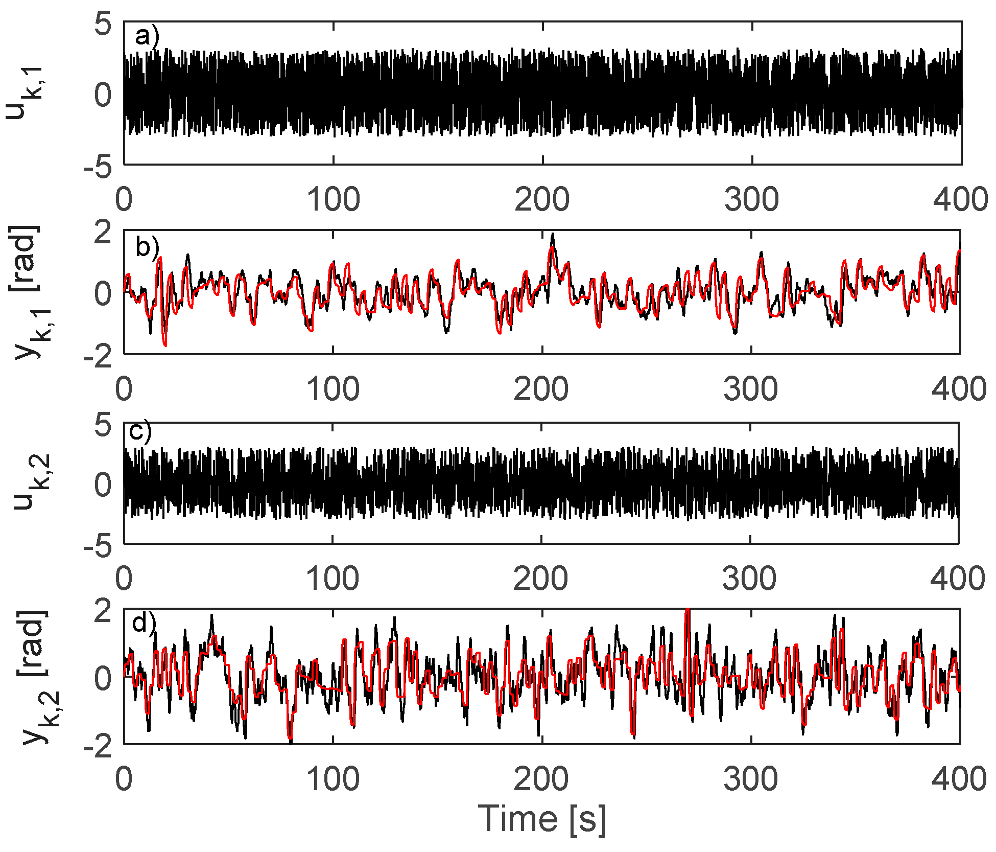
4. First Validation Case Study

A two-axis motion control system stemming from an aerial model is subjected to control learning via VSFRT and AI-VIRL. It is nonlinear and coupled and allows for vertical and horizontal positioning, being described as

$$\begin{array}{l}\{\begin{array}{l}{\dot{s}}_{a,1}=\left(S_{-1}^1(u_1)-M_h(s_{a,1})\right)/2.7\times {10}^{-5},\\ s_{a,2}=\tau /\left(23.8\times {10}^{-3}\times {\cos }^2{s}_{p,3}+3\times {10}^{-3}\right),\\ \dot{\tau }=\left(0.216F_a(s_{a,1})\cos s_{p,3}-0.058s_{a,2}+0.0178S_{-1}^1(u_2)\cos s_{p,3}\right),\\ {\dot{s}}_{a,3}=s_{a,2},\end{array}\\ \{\begin{array}{l}{\dot{s}}_{p,1}=\left(S_{-1}^1(u_2)-M_p(s_{p,1})\right)/1.63\times {10}^{-4},\\ {\dot{s}}_{p,2}=33.33\left(\begin{array}{l}0.2F_p(s_{p,1})-0.0127s_{p,2}-0.0935\sin s_{p,3}-\\ 9.28\times {10}^{-6}{s}_{p,2}\left|s_{p,1}\right|+4.17\times {10}^{-3}{S}_{-1}^1(u_1)-0.05\cos s_{p,3}\\ -0.021s_{a,2}^2\sin s_{p,3}\cos s_{p,3}+0.05\end{array}\right),\\ {\dot{s}}_{p,3}={\Omega }_p,\end{array}\end{array}$$

(13)

where $S_{-1}^1()$ means saturating function on $[-1,1]$, $u_1,u_2$ are the horizontal motion control input and the vertical motion control input respectively. $s_{a,3}(rad)=y_1\in [-\pi ,\pi ]$ is the horizontal angle, $s_{p,3}(rad)=y_2\in [-\pi /2,\pi /2]$ is the vertical angle, other states being described in [48]. The nonlinear static maps $M_p(s_{p,1}),F_p(s_{p,1}),M_a(s_{a,1}),F_a(s_{a,1})$ are fitted polynomials obtained for $s_{p,1},s_{a,1}\in (-4000;4000)$ [48].

A zero-order hold on the inputs combined with an outputs sampler applied on (13), conducts to an equivalent discrete-time model of relative degree one suitable for IO data collection and control. The system’s unknown dynamics will not be employed herein for learning control.

The objective of the problem (4) is here translated to finding the controller which makes the system’s outputs track the outputs of the LRM given as ${\mathbf{T}}_{LRM}(q)=diag(T\prime (q),T″(q))$ with $T\prime (q),T″(q)$ the discrete-time variants of $T\prime (s)=T″(s)=1/(\tau s+1),\tau =3$ obtained for the sampling interval of $\mathsf{\Delta }=0.1s$.

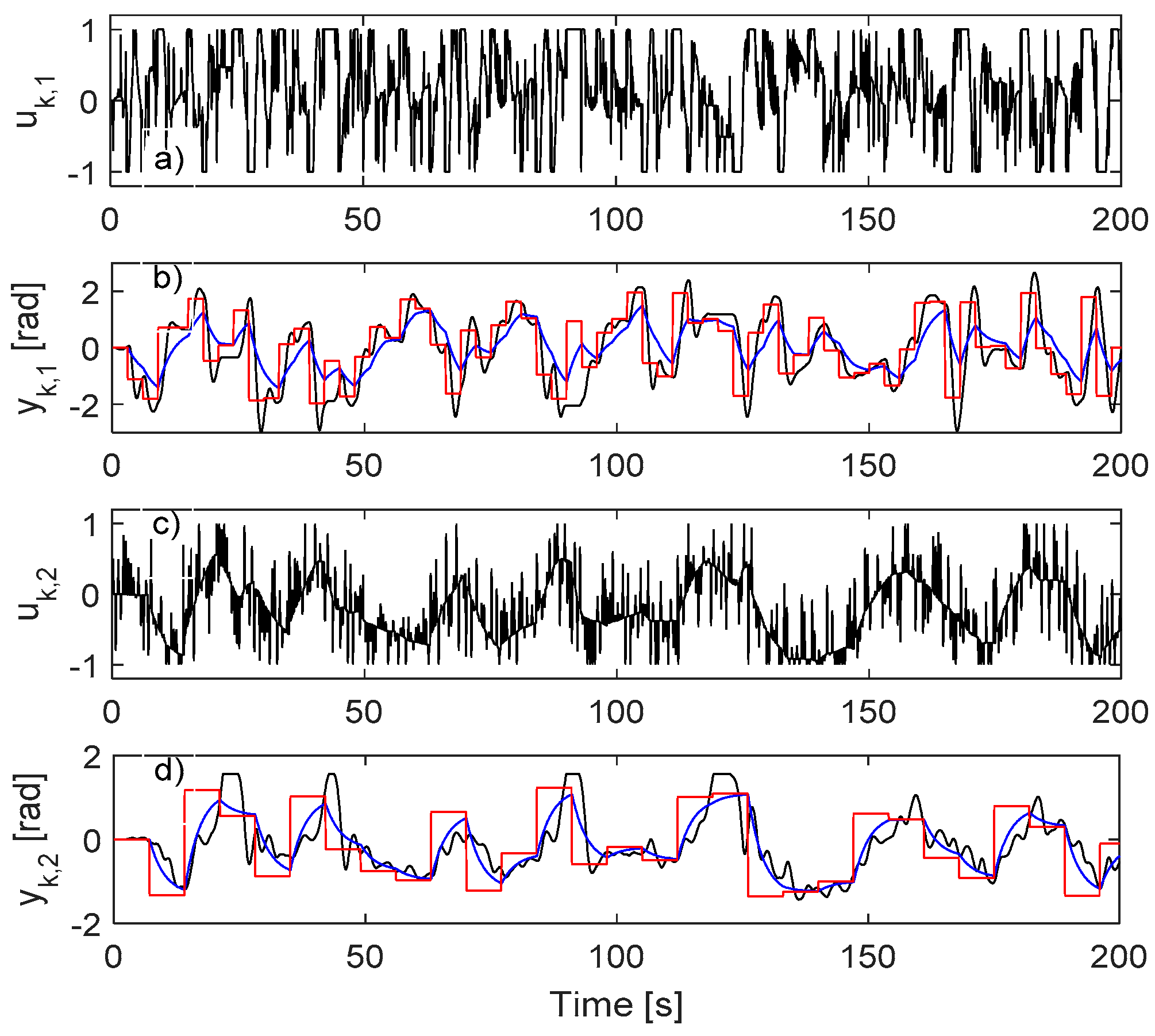
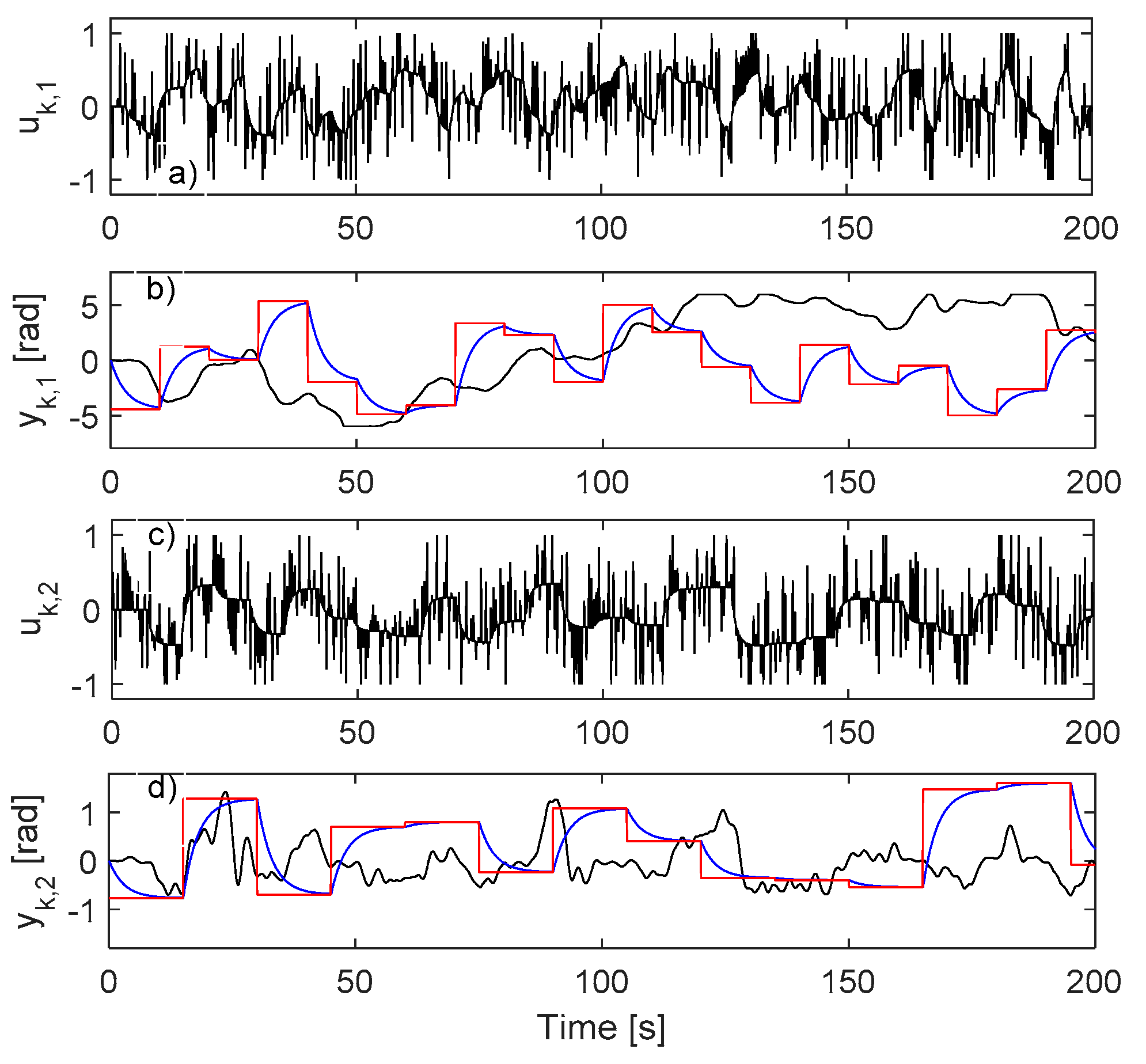
4.1. IO Data Collected in Closed-Loop

An initial linear MIMO IO controller is first found based on an IO variant of VRFT. The linear diagonal controller learned with IO VRFT is

$$\begin{gathered} C\left(q\right)=\frac{1}{D(q)}\left[\begin{array}{cc}{C}_{11}(q)& 0\\ 0& C_{22}(q)\end{array}\right], \\ \begin{array}{l}{C}_{11}(q)=2.6674-5.3354q^{-1}+3.5730q^{-2}-0.0339q^{-3}+0.0706q^{-4},\\ C_{22}(q)=0.5662-1.0491q^{-1}+0.4970q^{-2},\\ D(q)=1-q^{-1}.\end{array} \end{gathered}$$

(14)

For exploration enhancement, the reference inputs have their amplitudes uniformly randomly distributed in $r_{k,1}\in [-2;2],r_{k,2}\in [-1.4;1.4]$ and they present as piece-wise constant sequences of 3 s and 7 s, respectively. Every $5^{th}$ sampling instant, a uniform random number in $[-1;1]$ is added to the system inputs $u_{k,1},u_{k,2}$. Then $r_k$ drives the LRM

$$\{\begin{array}{c}{s}_{k+1,1}^m=0.9672s_{k,1}^m+0.03278r_{k,1},\\ s_{k+1,2}^m=0.9672s_{k,2}^m+0.03278r_{k,2},\\ y_k^m={[y_{k,1}^m{y}_{k,2}^m]}^T={[s_{k,1}^m{s}_{k,2}^m]}^T.\end{array}$$

(15)

With controller (14) in closed-loop over the output feedback error $u_{\mathrm{k}}=C(q)(r_k-y_k)$, IO data $\{u_{\mathrm{k}},y_k\}$ is collected for 2000 s, as rendered in Figure 1 (only for the first 200 s).

4.2. Learning the VSFRT Controller from Closed-Loop IO Data

Using the collected output data $y_{\mathrm{k}}$ and the given reference model $T_{LRM}(q)$, the virtual reference input is computed as ${\tilde{r}}_k=T_{LRM}^{-1}(q)y_k$. Afterwards, the extended state is built form the IO database $\{u_k,y_k\}$ and from ${\tilde{r}}_k$, as lumped in ${\tilde{s}}_k^{ex-}={[y_{k,1}{y}_{k,2}\dots y_{k-3,1}{y}_{k-3,2}{u}_{k-1,1}{u}_{k-1,2}{\tilde{r}}_{k,1}{\tilde{r}}_{k,2}]}^T$.

The extended state ${\tilde{s}}_k^{ex-}$ fills a database of the form $DS=\{({\tilde{s}}_k^{ex-},u_k^{})\}$ and it is used to learn the VSFRT NN controller using the VSFRT algorithm. The NN settings are described in

Table 1. Virtual State-feedback Reference Feedback Tuning (VSFRT) C-NN settings.

Setting	C-NN
Architecture	12-6-2 (12 inputs for $s_k^{ex}\in {\Re }^{12}$, 6 hidden layer neurons and 2 outputs: $u_{k,1},u_{k,2}$)
Activation function in hidden layer	tansig
Activation function in output layer	linear
Initial weights	uniform random numbers in [0;1]
Training algorithm	scaled conjugate gradient
Maximum number of epochs to train	100
Validation/training ratio	10–90%
Maximum validation failures	50
Minimum performance gradient	${10}^{-30}$
Training cost function	mean sum of squared errors (MSSE)

. Each learning trial trains the C-NN for $MaxTrain=200$ times, starting with reinitialized weights. Each trained C-NN was tested on the standard scenario shown in Figure 2 (only for the first 600 s), by measuring a normalized c.f. $V=1/N\cdot V_{LRMO}^N$ for $N=\mathrm{12,000}$ samples in 1200 s. The best C-NN (in terms of the minimal value of V per trial) is retained at each trial. One trial lasts about 30 min on a standard desktop computer with all calculations performed on CPU.

For a fair evaluation, the learning process is repeated for five trials. In

Table 2. VSFRT and Approximate Iterative Value Iteration Reinforcement Learning (AI-VIRL) tracking performance when learning uses closed-loop IO data.

Trial	VSFRT	AI-VIRL (500 Epochs)	AI-VIRL (100 Epochs)
1	0.0058104	0.010102	0.0070567
2	0.0054775	0.0066765	0.017531
3	0.0051332	0.0039271	0.034047
4	0.0092913	0.024098	0.01389
5	0.0058103	0.0069556	0.013097
Average	0.00630454	0.01035184	0.03424868

, the value of $V$ for five trials is filled and then averaged. The best C-NN, found in trial 3, has $V=0.0051332$.

4.3. Learning the AI-VIRL Controller from Closed-Loop IO Data

In this case, the extended state used to learn C-NN with AI-VIRL, built using the same dataset $\{u_k,y_k\}$, the states from the reference model $s_k^m$ and the reference input $r_k$, is $s_k^{ex}={[y_{k,1}{y}_{k,2}\dots y_{k-3,1}{y}_{k-3,2}{u}_{k-1,1},u_{k-1,2},r_{k,1},r_{k,2},s_{k,1}^m,s_{k,2}^m]}^T$.

Before using the raw database, the transition samples at time instants where $r_k\ne r_{k+1}$ are to be deleted (the piecewise constant step model is not a valid state-space at switching instants) and the resulted database used for learning is $DB=\{(s_k^{ex[i]},u_k^{[i]},s_{k+1}^{ex[i]})\},i=\overline{1,P},whereP<N$.

The controller NN and the Q-function NN settings are depicted in

Table 3. AI-VIRL C-NN and Q-NN settings.

Setting	C-NN	Q-NN
Architecture	14-10-2	16-30-1
Activation function in hidden layer	tansig	tansig
Activation function in output layer	linear	linear
Initial weights	uniform random numbers in [0;1]	uniform random numbers in [0;1]
Training algorithm	scaled conjugate gradient	scaled conjugate gradient
Maximum number of epochs to train	500 or 100	500
Validation/training ratio	10–90%	10–90%
Maximum validation failures	50	50
Minimum performance gradient	${10}^{-30}$	${10}^{-30}$
Training cost function	MSSE	MSSE

.

To find Q-NN’s minimizers for training the C-NN in Step 3 of the AI-VIRL algorithm, all possible input combinations $u_{k,1}\times u_{k,2}$ resulted from 19 discrete values in [–1;1] for each input are enumerated, for each $s_k^{ex[i]}$. The minimizing combination is set as target for the C-NN, for the given input $s_k^{ex[i]}$, at the current algorithm iteration.

Each AI-VIRL iteration produces a C-NN that is tested on the same standard test scenario used with VSFRT, by measuring a finite-time normalized c.f. $V=1/N\cdot V_{LRMO}^N$ for $N=\mathrm{12,000}$ samples over 1200 s. The AI-VIRL is iterated for $MaxIter=1000$ times and all stabilizing controllers that are better than the previous ones running on the standard test scenario are recorded. For fair evaluation, AI-VIRL is also run for five trials.

Two cases are analyzed, to test the impact of the training epochs on the controller NN. In the first case, both C-NN and Q-NN are to be trained for maximum 500 epochs. The best C-NN is found at iteration 822 of trial 3 and measures $V=0.0039271$ on the standard test scenario shown in Figure 3 (only the first 600 s shown).

In the second case, the Q-NN is trained for maximum 500 epochs and the C-NN is trained for maximum 100 epochs. The best C-NN is found at iteration 573 of the first trial and measures $V=0.0070567$ on the standard test scenario shown in Figure 4 (only the first 600 s shown).

The iterative learning process specific to AI-VIRL lasts for approximately 6 h in the first above mentioned case and for about 4 h in the second case, on a standard desktop computer with all operations on CPU. All measurements corresponding to the five trials in the two cases are filled in Table 2.

After learning the AI-VIRL control, the conclusion w.r.t. VSFRT learned control can be drawn: The VSFRT control is computationally cheaper to learn (one-shot instead of iterative) and the average tracking control performance is better with VSFRT (about an order of magnitude better).

4.4. Learning VSFRT and AI-VIRL Control Using IO Data Collected in Open-Loop

Next, we repeat the learning process for the two controllers (the VSFRT one and the AI-VIRL one) but the data used for learning is collected in open-loop as depicted in Figure 5. For the sake of exploration, the system inputs have their amplitudes uniformly randomly distributed in $u_{k,1}\in [-0.45;0.6],u_{k,2}\in [-0.5;0.4]$ and they present as piece-wise constant sequences of 3 s and 7 s, respectively. Each of $u_{k,1},u_{k,2}$ are firstly filtered through the lowpass dynamics 1/(s+1). Then every $5^{th}$ sampling instant, a uniform random number in $[-1;1]$ is again added to the filtered $u_{k,1},u_{k,2}$. A crucial difference w.r.t. the closed-loop collection scenario is that the reference inputs drive only the LRM and since there is no controller in closed-loop, the reference inputs $r_k$ and the LRM’s outputs $y_k^m=T_{LRM}(q)r_k$ evolve as correlated but independently of the system outputs who were excited by $u_k$. For exploration, the reference inputs have their amplitudes uniformly randomly distributed in $r_{k,1}\in [-6;6],r_{k,2}\in [-1;2]$ and they are also piece-wise constant sequences of 10 and 15 s, respectively. We underline that for VSFRT, $r_k$ and $y_k^m$ are not needed as they are automatically offline calculated by the VSFRT principle. However, AI-VIRL uses them for forming the extended state-space model.

It is clear when comparing Figure 1 with Figure 5 that the open-loop data collection in uncontrolled environment is not satisfactorily exploring the input-state space (there is significantly less variation in the outputs). This may affect learning convergence and final LRM tracking performance.

The extended states for VSFRT and AI-VIRL and their NNs settings are kept the same as in the closed-loop IO collection scenario.

For a fair evaluation, the learning process is repeated five times for all the cases previously described. In

Table 4. VSFRT and AI-VIRL tracking performance when learning uses open-loop IO data.

Trial	VSFRT	AI-VIRL (500 Epochs)	AI-VIRL (100 Epochs)
1	0.0057742	1.6159	1.0426
2	0.004507	0.24	0.96942
3	0.0055276	1.8268	1.0055
4	0.0043692	0.63566	1.3044
5	0.0049202	0.84485	0.20267
Average	0.00501964	1.032642	0.904918

is noted the value of $V$ for each trial and the average value.

The best VSFRT controller, obtained in trial 4, measures $V=0.0043692$ on the test scenario from Figure 6, a value close to the minimal value obtained in the closed-loop IO data collection scenario. The AI-VIRL controllers’ performance is obviously inferior; the C-NN with the minimal V in the case when it is trained for maximum 100 epochs, is found at iteration 15 and measures $V=0.24$ on the second trial (tracking is shown in Figure 7 the first 600 s only); the C-NN with minimal V (best tracking) in the case when trained for maximum 500 epochs, is found at iteration 132 of the fifth trial and measures $V=0.20267$ on the standard test scenario shown in Figure 8 for the first 600 s only.

The conclusion is that the poor exploration fails the AI-VIRL convergence to a good controller, whereas the VSFRT controller is learned to about the same LRM tracking performance. VSFRT learns better control (about two order of magnitude smaller V than with AI-VIRL) while being less computationally demanding and despite the poor exploration.

4.5. Testing the Transfer Learning Advantage

It is checked whether initializing the AI-VIRL algorithm with an admissible VSFRT controller helps improving the learning convergence, using the transfer learning capability. An initial admissible controller is not however mandatory for the AI-VIRL. Since both the VSFRT and the AI-VIRL controllers aim at solving the same LRMO tracking control problem, it is expected that the VSFRT controller initializes AI-VIRL closer to the optimal controller.

The VSFRT controller from the closed-loop IO data collection case is transferred since this case has proved good LRMO tracking for both the VSFRT and for the AI-VIRL controllers. Two cases were again analyzed: When the C-NN of the AI-VIRL is trained for 100 epochs at each iteration and when the C-NN of the AI-VIRL is trained for 500 epochs at each iteration. While the Q-NN has its weights randomly initialized with each trial.

The results unveil that the transfer learning does not speed up the AI-VIRL convergence, nor does it result in better AI-VIRL controllers after the trial ends. The reason is that the learning process taking place in the high-dimensional space spanned by the C-NN weights remains un-controllable directly, but only indirectly by the hyper-parameter settings such as database exploration quality and size, training overfitting prevention mechanism and adequate NN architecture setup.

4.6. VSFRT and AI-VIRL Performance under State Dimensionality Reduction with PCA and Autoencoders

State representation is a notorious problem in approximate dynamic programming and reinforcement learning. In the observability-based framework, the state comprises of past IO samples who are time-correlated. Meaning that the desired uniform coverage of the state space is significantly affected. Intuitively, the more recent IO samples from the virtual state better reflect the actual system state, whereas the older IO samples are less characterizing the actual system state.

Analyzing the state representation for VSFRT and for AI-VIRL, two sources of correlation appear. First, the time-correlation since the virtual state is constructed from past IO samples. Secondly, correlation appears between the independent reference inputs (used in closed-loop IO data collection) and the LRM’s states and outputs and the system’s inputs and outputs as well. It is therefore justified to strive for state dimensionality reduction.

One of the popular unsupervised machine learning tools for dimensionality reduction is principal component analysis (PCA). Thanks to its offline nature, it can be used only with offline learning schemes, such as VSFRT and AI-VIRL. Let the state vector $s_k^{}$ recordings be arranged in a matrix S where the number of columns correspond to the state components and the line number is the record time index k. The state $s_k^{}$ can be either one of ${\tilde{s}}_k^{ex-}$ for VSFRT or $s_k^{ex}$ for AI-VIRL. Let the empirical estimate of the covariance of S be $\tilde{S}$ obtained after centering the columns of S to zero, and the square matrix V contains $\tilde{S}$’s eigenvectors on each column, arranged from the left to the right, in the descending order of the eigenvalues amplitudes. The number $n_P$ of principal components counts the first $n_P$ leftmost columns from V, which are the principal components. Let this leftmost slicing of V be $V^L$. The reduced represented state is then calculated as $s^{red}={(V^L)}^{T}s$.

The state dimensionality reduction effect on tracking performance is tested both for the VSFRT and for the AI-VIRL. The used database is the one from the closed-loop collection scenario since this offers a learning chance to both VSFRT and to the AI-VIRL controllers. For VSFRT, the dimension of the state ${\tilde{s}}_k^{ex-}$ is 12, whereas for AI-VIRL, the dimension of $s_k^{ex}$ is 14. For VSFRT, the first 4 principal components explain for 98.32% of the data variation, while for AI-VIRL, the first 6 components explain for 98.51% of the data variation, confirming existent high correlations between the state vector components. This leads to reduced C-NN architecture sizes of 4–6–2 for VSFRT and 6–6–2 for AI-VIRL. For AI-VIRL, the case where 100 epochs for training the C-NN was employed. The explained variation in the data is shown for the first four principal components only for VSFRT, in Figure 9.

The best learned C-NN with VSFRT and with AI-VIRL measure $V=0.1653$ and $V=1.3488$ respectively, on the test scenario. The VSFRT controller performs well only on controlling $y_{k,1}$ while poorly on controlling $y_{k,2}$. Whereas the AI-VIRL control is unexploitable on any of the two axes. The conclusion is that the exploration issue is exacerbated by the state dimensionality reduction, although learning still takes place to some extent. Even when the data variation is explainable by a reduced number of principal components, due to many apparent correlations.

Under reduced state information loss when performing dimensionality reduction, no improvement on the best tracking performance is expected. However, learning still occurs, which encourages to use the dimensionality reduction as a trade-off for reducing learning computational effort by reducing the state space size and subsequently the NN architecture size.

A standard fully-connected single-hidden layer feedforward autoencoder (AE) is next used to test the dimensionality reduction and its effect on the learning performance, in a different unsupervised machine learning paradigm. Details of the autoencoder are: Six hidden neurons that are the encoder’s outputs and is also the number of reduced features; sigmoidal activation function from the input-to-hidden layer as well as from the hidden-to-output layer; number of training epochs set to maximum 500. The training cost function is of the form $T_{MSSE}+c_1{T}_{L_2}+c_2{T}_{sparse}$ where $T_{MSSE}$ penalizes the mean summed squared deviation of the AE outputs from the same inputs, $T_{L_2}$ is the weights L₂ regularization term responsible with limiting the AE weights amplitude and the $T_{sparse}$ term encourages sparsity at the AE hidden layer’s output. $T_{sparse}$ measures the Kullback–Leibler divergence of the averaged hidden layer outputs activation values with respect to a desirable value set as 0.15 in this case study. While the other parameters in the cost are set as $c_1=0.004,c_2=4$. The AE’s targeted output is the copied input.

The AE-based dimensionality reduction is only applied to the VSFRT control learning. Let the encoder map the input to the dimensionally-reduced feature as in ${\tilde{s}}_k^{red}=Enc({\tilde{s}}_k^{ex-})$. The VSFRT C-NN training now uses the pairs $\{{\tilde{s}}_k^{red},u_k\}$ using the same value $MaxTrain=200$ and the same five trials approach. The best learned C-NN with VSFRT measured $V=0.1838$ which is on par with the best performance from the VSFRT C-NN learned with PCA reduction. The result unveils that no significant improvement is obtained using the AE-based reduction, which is expected due to sensible information loss. Then there is no preference for using either of PCA or AE for this purpose. It also confirms that no better performance is attainable. However, it is advised to use dimensionality reduction tools since by a reduced virtual state, simpler (as in reduced number of parameters) NN architectures are usable, leading to less computational effort in training, testing and real-world implementation phase.

5. Second Validation Case Study

A two-joints rigid and planar robot arm serves in the following case study. Its dynamics are described by [49]

$$m_1(s)\ddot{s}+m_2(s,\dot{s})\dot{s}=Sat(u)$$

(16)

where $u={[u_1,u_2]}^T$ are motor input torques for the base joint and for the tip joint, respectively. Both inputs are limited inside the model, within their domains [−0.2; 0.2] Nm and [−0.1; 0.1] Nm, respectively, through the component-wise saturation function $Sat(•)$. $s={[s_1,s_2]}^T$ measured in radians (rad) represents the angle of the base and tip joints, respectively. While the joints’ angular velocities which are unmeasurable are captured in $\dot{s}={[{\dot{s}}_1=s_3,{\dot{s}}_2=s_4]}^T$ and physically limited inside $[-2\pi ,2\pi ]$ rad/s. When no gravitational forces affect the planar arm, the matrices in the Equation (16) are

$$\begin{array}{l}{m}_1(s)=\left[\begin{array}{cc}{m}_1{c}_1^2+m_2{l}_1^2+I_1+m_2{c}_2^2+I_2+2m_2{l}_1{c}_2\cos s_2& m_2{c}_2^2+I_2+m_2{l}_1{c}_2\cos s_2\\ m_2{c}_2^2+I_2+m_2{l}_1{c}_2\cos s_2& m_2{c}_2^2+I_2\end{array}\right],\\ m_2(s,\dot{s})=\left[\begin{array}{cc}{b}_1-m_2{l}_1{c}_2{s}_4\sin s_2& -m_2{l}_1{c}_2(s_3+s_4)\sin s_2\\ m_2{l}_1{c}_2{x}_3\sin s_2& b_2\end{array}\right],\end{array}$$

(17)

with the parameters’ numerical values set as l₁ = 0.1, l₂ = 0.1, m₁ = 1.25, m₂ = 1, I₁ = 0.004, I₂ = 0.003, c₁ = 0.05, c₂ = 0.05, b₁ = 0.1, b₂ = 0.02. These parameters’ interpretation is irrelevant to the following developments.

A sample period $\mathsf{\Delta }=0.05s$ characterizes a zero-order hold applied on the inputs and on the outputs of (16), rendering it into an equivalent discrete-time model with inputs $u_k={[u_{k,1},u_{k,2}]}^T$ and outputs $y_k={[y_{k,1}=s_{k,1},y_{k,2}=s_{k,2}]}^T$.

It is intended to search for the control which makes the closed-loop match the continuous-time decoupled LRM model $T_{LRM}(s)=diag(1/(0.5s+1),1/(0.2s+1))$, which is subsequently transformed to the discrete-time observable canonical state-space form

$$\{\begin{array}{l}{s}_{k+1,1}^m=0.9048s_{k,1}^m+0.0952r_{k,1}^{},\\ s_{k+1,2}^m=0.7788s_{k,2}^m+0.2212r_{k,2}^{},\\ y_k^m={[y_{k,1}^m{y}_{k,2}^m]}^T={[s_{k,1}^m{s}_{k,2}^m]}^T.\end{array}$$

(18)

$T_{LRM}(q)$ is the discrete-time counterpart of $T_{LRM}(s)$, calculated for the sample period $\mathsf{\Delta }$.

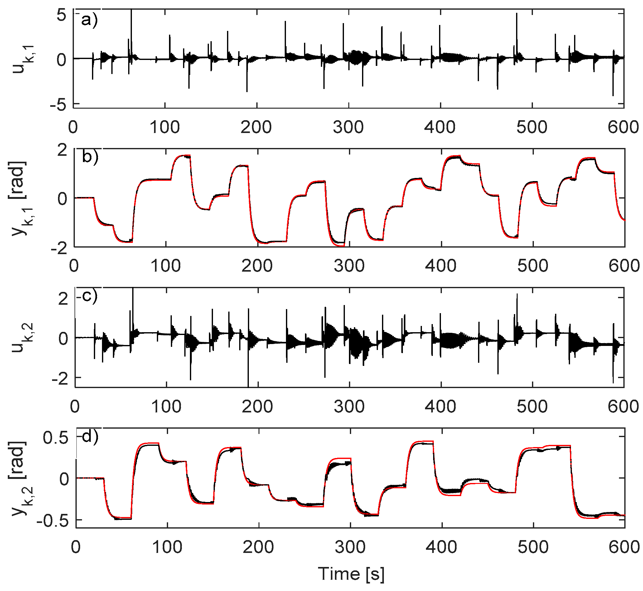
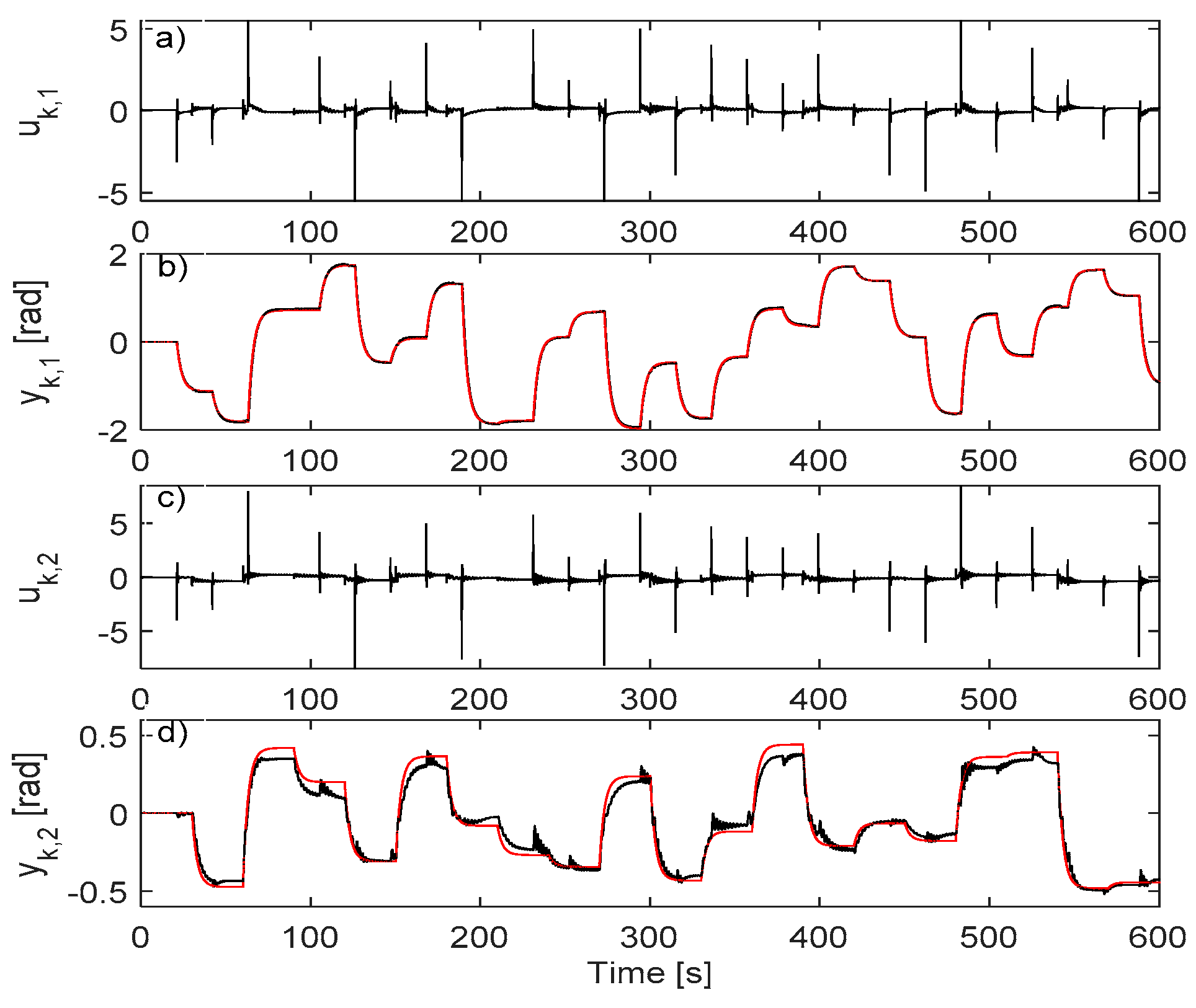
5.1. IO Data Collection in Closed-Loop

The transition samples must be collected first. Initial non-decoupling proportional-type controllers are used, given as u_k,1 = 0.15 × (r_k,1 − y_k,1) and u_k,2 = 0.05 × (r_k,2 − y_k,2), respectively.

For driving the resulted closed-loop CS, r_k,1 is modeled as a sequence of piecewise constant values for 2 s with zero-mean random amplitudes of variance 0.6 and r_k,2 is as a sequence of piecewise constant values for 1 s with zero-mean random amplitudes of variance 0.65. For enhanced exploration, random additive disturbance is used on inputs $u_{k,1},u_{k,2}.$ A uniform random number in $[-3,3]$ is added to the first input every 2nd sample and a similar distribution random number is added to the second input every 3rd sample. A total of 15,000 samples of $r_{k,1},r_{k,2},u_{k,1},u_{k,2},y_{k,1},y_{k,2},y_{k,1}^m,y_{k,2}^m$ are collected. The collection is shown in Figure 10.

5.2. Learning the VSFRT Controller from Closed-Loop IO Data

Using the collected output data $y_{\mathrm{k}}$ and the given reference model $T_{LRM}(q)$, the virtual reference input is computed as ${\tilde{r}}_k=T_{LRM}^{-1}(q)y_k$. Afterwards, the extended state is built form the IO database samples $\{u_k,y_k\}$ and from ${\tilde{r}}_k$, all components being lumped in ${\tilde{s}}_k^{ex-}={[y_{k,1}{y}_{k,2}{y}_{k-1,1}{y}_{k-1,2}{y}_{k-2,1}{y}_{k-2,2}{u}_{k-1,1}{u}_{k-1,2}{\tilde{r}}_{k,1}{\tilde{r}}_{k,2}]}^T$.

The extended state ${\tilde{s}}_k^{ex-}$ fills a database of the form $DB=\{({\tilde{s}}_k^{ex-},u_k^{})\}$ and it is used to learn the VSFRT NN controller according to the VSFRT algorithm. The C-NN settings are described in

Table 5. VSFRT C-NN settings.

Setting	C-NN
Architecture	10-6-2
Activation function in hidden layer	tansig
Activation function in output layer	linear
Initial weights	uniform random numbers in [0;1]
Training algorithm	scaled conjugate gradient
Maximum number of epochs to train	100
Validation/training ratio	10–90%
Maximum validation failures	50
Minimum performance gradient	${10}^{-30}$
Training cost function	MSSE

. Each learning trial trains the C-NN for $MaxSteps=200$ times, starting with reinitialized weights. Each trained C-NN was tested in closed-loop on a scenario where the test reference inputs are identical to those used in Figure 11, by measuring a normalized c.f. $V=1/N\cdot V_{LRMO}^N$ for $N=400$ samples in 20 s. The best C-NN (in terms of the minimal value of V per trial) is retained at each trial. One trial lasts about 30 min on a standard desktop computer with all calculations performed on CPU. For a fair evaluation, the learning process is repeated for five trials. In

Table 6. VSFRT and AI-VIRL tracking performance when learning uses closed-loop IO data.

Trial	VSFRT	AI-VIRL (500 Epochs)
1	0.0043144	0.0039152
2	0.0050468	0.0051058
3	0.0040801	0.0068728
4	0.0044891	0.0058930
5	0.0045807	0.0055730
Average	0.0045022	0.0054719

, the value of $V$ for five trials is filled and then averaged. About 95% of the learned controllers are stabilizing, in spite of the underlying nonlinear optimization specific to VSFRT, indirectly solved by C-NN training.

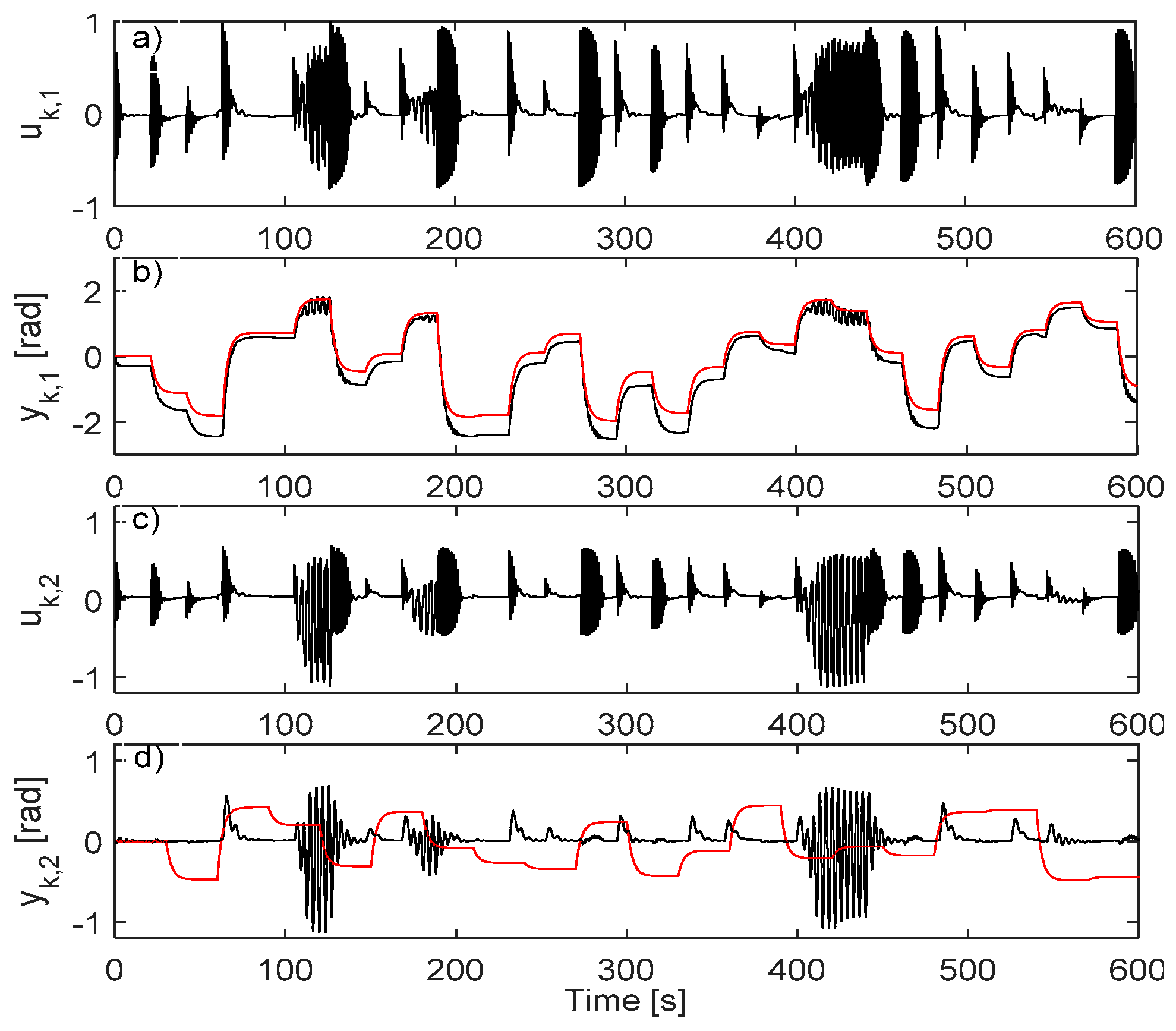
5.3. Learning the AI-VIRL Controller from Closed-Loop IO Data

The extended state used to learn C-NN with AI-VIRL, built using the same database $\{u_k,y_k\}$ collected for VSFRT, together with the states from the reference model $s_k^m$ and the reference input $r_k$. The extended state vector is comprised of $s_k^{ex}={[y_{k,1}{y}_{k,2}{y}_{k-1,1}{y}_{k-1,2}{y}_{k-2,1}{y}_{k-2,2}{u}_{k-1,1},u_{k-1,2},r_{k,1},r_{k,2},x_{k,1}^m,x_{k,2}^m]}^T$.

Before using the raw database, the transition samples at time instants where $r_k\ne r_{k+1}$ are to be excluded (the piecewise constant step model is not a valid state-space transition model at switching instants) and the resulted database used for learning is $DB=\{(s_k^{ex[i]},u_k^{[i]},s_{k+1}^{ex[i]})\},i=\overline{1,P},whereP<N$.

The controller NN and the Q function NN settings are depicted in

Table 7. AI-VIRL C-NN and Q-NN settings.

Setting	C-NN	Q-NN
Architecture	12-6-2	14-40-1
Activation function in hidden layer	tansig	tansig
Activation function in output layer	linear	linear
Initial weights	uniform random numbers in [0;1]	uniform random numbers in [0;1]
Training algorithm	scaled conjugate gradient	scaled conjugate gradient
Maximum number of epochs to train	100	500
Validation/training ratio	10–90%	10–90%
Maximum validation failures	50	50
Minimum performance gradient	${10}^{-30}$	${10}^{-30}$
Training cost function	MSSE	MSSE

.

To find Q-NN’s minimizers for training the C-NN in Step 3 of the AI-VIRL algorithm, all possible input combinations $u_{\mathrm{k},1}\times u_{k,2}$ resulted from 25 discrete values in [−2;2] for each input are enumerated, for each $s_k^{ex[i]}$. The minimizing combination is set as target for the C-NN, for the given input $s_k^{ex[i]}$, at the current algorithm iteration.

Each AI-VIRL iteration produces a C-NN that is tested on the same standard test scenario used with VSFRT, by measuring the c.f. $V$ for $N=400$ samples over 20 s. The AI-VIRL is iterated $MaxIter=200$ times and all stabilizing controllers that are better than the previous ones running on the standard test scenario are recorded. For fair evaluation, AI-VIRL is also run for five trials and all the best measurements over one trial (and the average value per trials) are filled in Table 6.

After learning the AI-VIRL controllers, the conclusion based on Table 6 is clear: VSFRT is again better than AI-VIRL, in spite of being computationally less demanding and also being one-shot. The learning took place on the same database, in a controlled environment where good exploration was attainable.

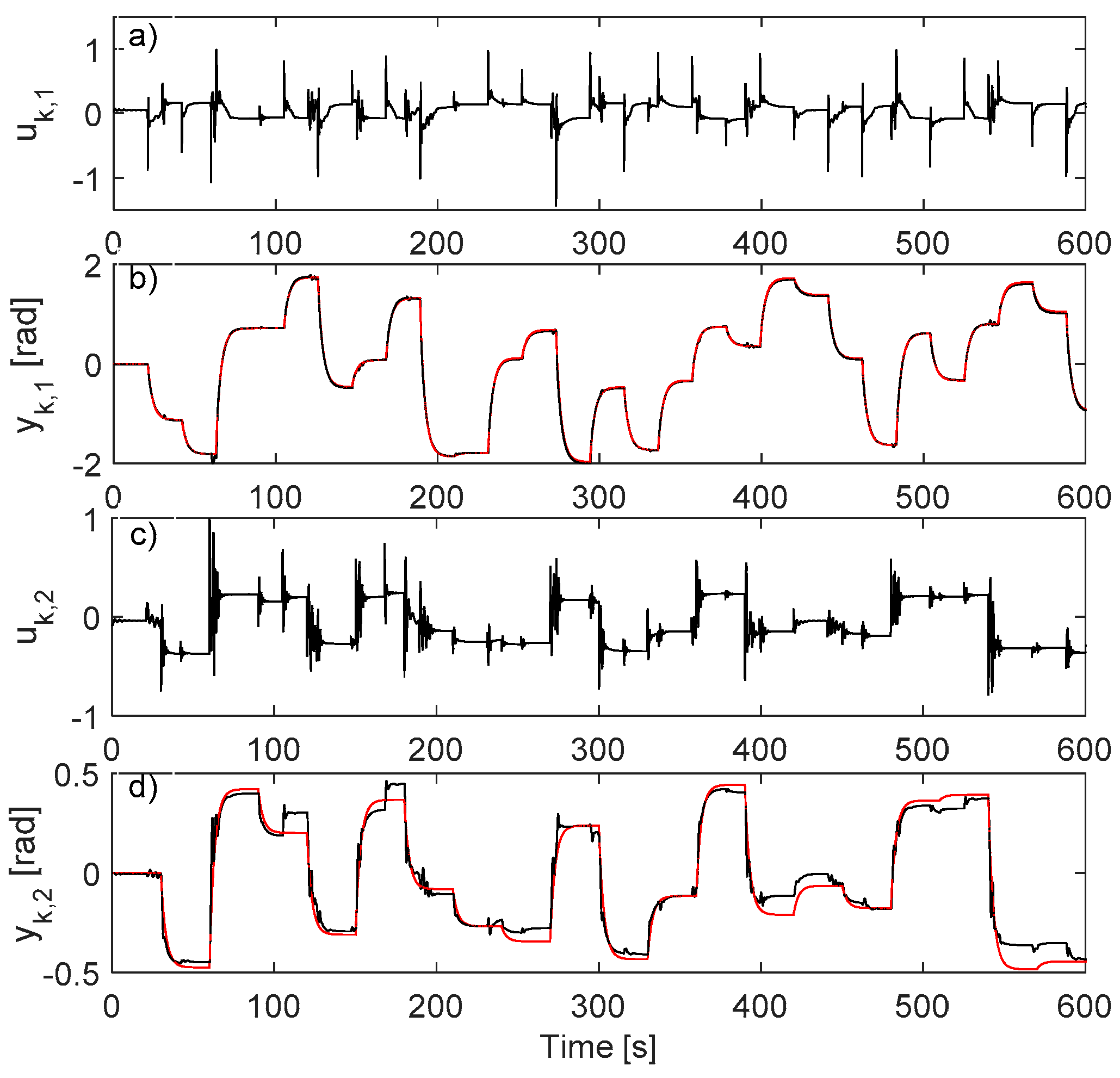
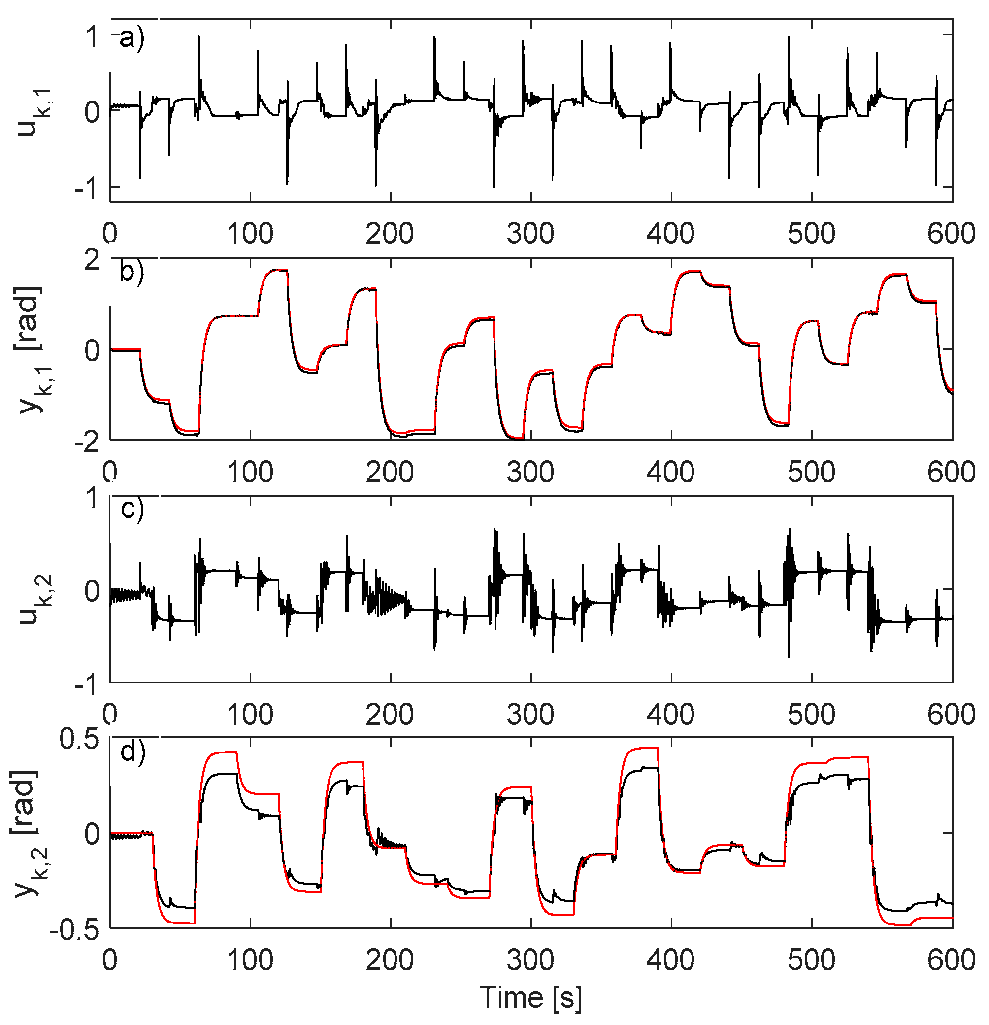
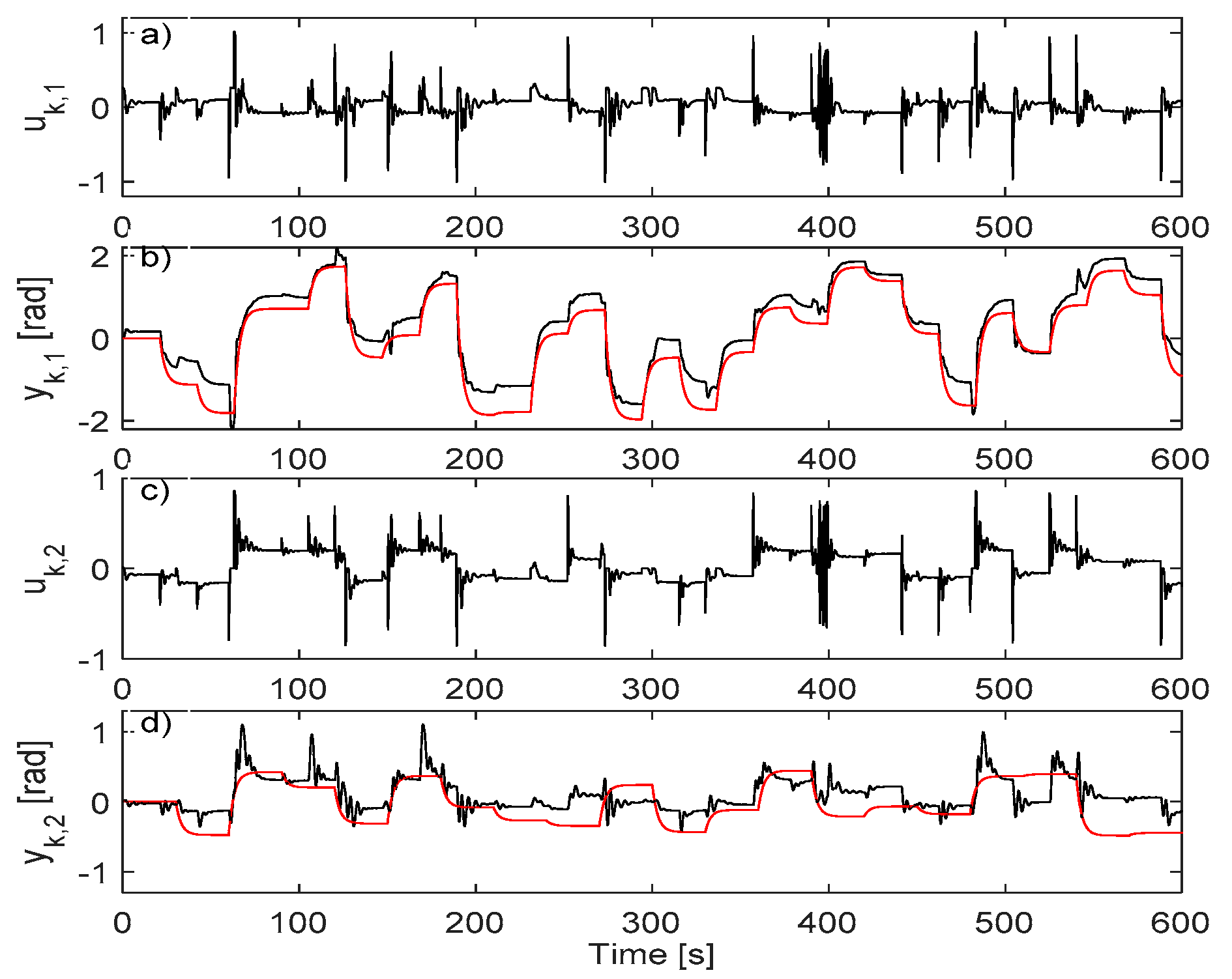
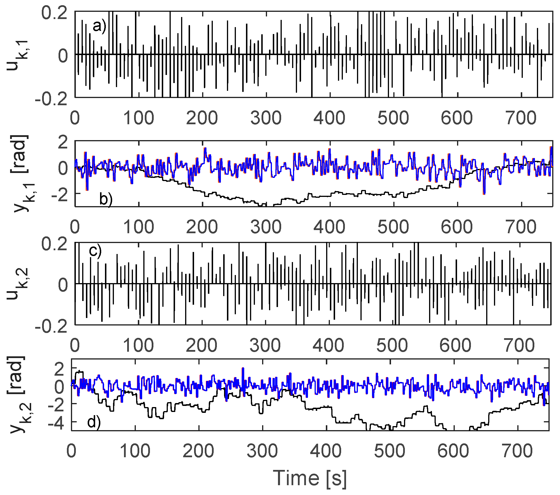
5.4. Learning VSFRT and AI-VIRL Control Based on IO Data Collected in Open-Loop

The robotic arm act as an open-loop integrator on each joint, hence being marginally stable. The open-loop collection is driven by zero-mean impulse inputs $u_{k,1},u_{k,2}$. For exploration’s sake, the reference inputs have their amplitudes uniformly randomly distributed in $r_{k,1}\in [-1.5;1.5],r_{k,2}\in [-2;2]$ and they present as sequences of piece-wise constant signals lasting 2.5 s and 2 s, respectively. The difference now w.r.t. the closed-loop collection scenario is that the reference inputs $r_k$ drive only the LRM and since there is no controller in closed-loop, the reference inputs and the LRM’s outputs $y_k^m=T_{LRM}(q)r_k$ evolve independently of the system’s outputs $y_k$ who were driven by $u_k$. The open-loop collection is captured in Figure 12 from where it is clear that $y_{k,1},y_{k,2}$ do not intersect too often with $r_{k,1},r_{k,2}$ and with $y_{k,1}^m,y_{k,2}^m$, respectively.

The exact same learning settings from the closed-loop case were used for VSFRT and for AI-VIRL. Notice that $r_{k,1},r_{k,2}$ and with $y_{k,1}^m,y_{k,2}^m$ are not used for learning control with VSFRT since they do not enter the extended state ${\tilde{s}}_k^{ex-}$.

Five learning trials are executed both for VSFRT and for AI-VIRL, with the LRMO tracking performance measure V recorded in

Table 8. VSFRT and AI-VIRL tracking performance when learning uses open-loop IO data.

Trial	VSFRT	AI-VIRL (100 Epochs)
1	0.0021623	0.127480
2	0.0021440	0.273590
3	0.0021695	0.865850
4	0.0021951	0.202360
5	0.0021497	0.175330
Average	0.0021641	0.328922

. The best learned VSFRT and AI-VIRL controllers are shown performing on the standard tracking test scenario in Figure 11.

There is a dramatic difference in favor of VSFRT’s superior tracking performance, in spite of the poorer input-state space exploration. As expected, AI-VIRL’s convergence to a good controller is affected by the poor exploration and its performance is not better than in the closed-loop collection case. Concluding, the superiority of VSFRT over AI-VIRL is again confirmed, both in terms of reduced computation complexity/time and in terms of tracking performance.

6. Conclusions

Learning controllers from IO data to achieve high LRM output tracking performance has been validated by both VSFRT and AI-VIRL. Learning takes place in the space of the new virtual state representation build from historical IO samples, to address observable systems. The resulted control is in fact learned to be applied to the original underlying system. Surprisingly in the two illustrated case studies, using the same IO data and the same LRM, VSFRT showed no worse tracking performance than AI-VIRL, despite its significantly lesser computation demands. While in the cases of poor exploration, VSFRT was clearly superior.

Aside performance comparisons, several additional studies were conducted. The transfer learning opportunity from VSFRT to provide initial admissible controller for the AI-VIRL showed no advantage. While transfer learning could theoretically accelerate the learning convergence to the optimal control, the result indicates that learning in the high-dimensional space spanned by the C-NN weights remains uncontrollable directly, but only indirectly by the hyper-parameter settings such as database exploration quality and size, training overfitting prevention mechanism and adequate NN architecture setup. Since the resulted state representation will generally lead to large virtual state vectors, the impact of dimensionality reduction through standard unsupervised machine learning techniques such as principal component analysis and autoencoders was studied. The obtained results indicate that no significant improvement is obtained, then there is no preference for using either one of PCA or AE for this purpose. It also confirms that no better tracking performance is attainable. However, it is advised to use dimensionality reduction since by a reduced virtual state, simpler (in the sense of fewer parameters) NN architectures are used, leading to less computational effort in training, testing and real-world implementation phase.

References

1. Fu, H.; Chen, X.; Wang, W.; Wu, M. MRAC for unknown discrete-time nonlinear systems based on supervised neural dynamic programming. Neurocomputing 2020, 384, 130–141. [Google Scholar] [CrossRef]
2. Wang, W.; Chen, X.; Fu, H.; Wu, M. Data-driven adaptive dynamic programming for partially observable nonzero-sum games via Q-learning method. Int. J. Syst. Sci. 2019, 50, 1338–1352. [Google Scholar] [CrossRef]
3. Perrusquia, A.; Yu, W. Neural H2 control using continuous-time reinforcement learning. IEEE Trans. Cybern. 2020, 1–10. [Google Scholar] [CrossRef]
4. Sardarmehni, T.; Heydari, A. Sub-optimal switching in anti-lock brake systems using approximate dynamic programming. IET Control Theory Appl. 2019, 13, 1413–1424. [Google Scholar] [CrossRef]
5. Martinez-Piazuelo, J.; Ochoa, D.E.; Quijano, N.; Giraldo, L.F. A multi-critic reinforcement learning method: An application to multi-tank water systems. IEEE Access 2020, 8, 173227–173238. [Google Scholar] [CrossRef]
6. Liu, Y.; Zhang, H.; Yu, R.; Xing, Z. H∞ tracking control of discrete-time system with delays via data-based adaptive dynamic programming. IEEE Trans. Syst. Man Cybern. Syst. 2020, 50, 4078–4085. [Google Scholar] [CrossRef]
7. Na, J.; Lv, Y.; Zhang, K.; Zhao, J. Adaptive identifier-critic-based optimal tracking control for nonlinear systems with experimental validation. IEEE Trans. Syst. Man. Cybern. Syst. 2020, 1–14. [Google Scholar] [CrossRef]
8. Li, J.; Ding, J.; Chai, T.; Lewis, F.L.; Jagannathan, S. Adaptive interleaved reinforcement learning: Robust stability of affine nonlinear systems with unknown uncertainty. IEEE Trans. Neural. Netw. Learn. Syst. 2020, 1–11. [Google Scholar] [CrossRef]
9. Buşoniu, L.; de Bruin, T.; Tolić, D.; Kober, J.; Palunko, I. Reinforcement learning for control: Performance, stability, and deep approximators. Annu. Rev. Control 2018, 46, 8–28. [Google Scholar] [CrossRef]
10. Treesatayapun, C. Knowledge-based reinforcement learning controller with fuzzy-rule network: Experimental validation. Neural Comput. Appl. 2020, 32, 9761–9775. [Google Scholar] [CrossRef]
11. Huang, M.; Liu, C.; He, X.; Ma, L.; Lu, Z.; Su, H. Reinforcement learning-based control for nonlinear discrete-time systems with unknown control directions and control constraints. Neurocomputing 2020, 402, 50–65. [Google Scholar] [CrossRef]
12. Chen, C.; Sun, W.; Zhao, G.; Peng, Y. Reinforcement Q-Learning incorporated with internal model method for output feedback tracking control of unknown linear systems. IEEE Access 2020, 8, 134456–134467. [Google Scholar] [CrossRef]
13. De Bruin, T.; Kober, J.; Tuyls, K.; Babuska, R. Integrating state representation learning into deep reinforcement learning. IEEE Robot. Autom. Lett. 2018, 3, 1394–1401. [Google Scholar] [CrossRef]
14. Mnih, V.; Kavukcuoglu, K.; Silver, D.; Rusu, A.A.; Veness, J.; Bellemare, M.G.; Graves, A.; Riedmiller, M.; Fidjeland, A.K.; Ostrovski, G.; et al. Human-level control through deep reinforcement learning. Nature 2015, 518, 529–533. [Google Scholar] [CrossRef]
15. Lewis, F.L.; Vamvoudakis, K.G. Reinforcement learning for partially observable dynamic processes: Adaptive Dynamic Programming using measured output data. IEEE Trans. Syst. Man. Cybern. B Cybern. 2011, 41, 14–25. [Google Scholar] [CrossRef]
16. Wang, Z.; Liu, D. Data-based controllability and observability analysis of linear discrete-time systems. IEEE Trans. Neural Netw. 2011, 22, 2388–2392. [Google Scholar] [CrossRef]
17. Ni, Z.; He, H.; Zhong, X. Experimental studies on data-driven heuristic dynamic programming for POMDP. Front. Intell. Control. Inf. Process. 2014, 83–105. [Google Scholar]
18. Ruelens, F.; Claessens, B.J.; Vandael, S.; De Schutter, B.; Babuska, R.; Belmans, R. Residential demand response of thermostatically controlled loads using batch reinforcement learning. IEEE Trans. Smart Grid 2017, 8, 2149–2159. [Google Scholar] [CrossRef] [Green Version]
19. Campi, M.C.; Lecchini, A.; Savaresi, S.M. Virtual reference feedback tuning: A direct method for the design of feedback controllers. Automatica 2002, 38, 1337–1346. [Google Scholar] [CrossRef] [Green Version]
20. Formentin, S.; Savaresi, S.M.; Del Re, L. Non-iterative direct data-driven controller tuning for multivariable systems: Theory and application. IET Control Theory Appl. 2012, 6, 1250. [Google Scholar] [CrossRef]
21. Campestrini, L.; Eckhard, D.; Gevers, M.; Bazanella, A.S. Virtual Reference Feedback Tuning for non-minimum phase plants. Automatica 2011, 47, 1778–1784. [Google Scholar] [CrossRef]
22. Eckhard, D.; Campestrini, L.; Christ Boeira, E. Virtual disturbance feedback tuning. IFAC J. Syst. Control 2018, 3, 23–29. [Google Scholar] [CrossRef]
23. Campi, M.C.; Savaresi, S.M. Direct nonlinear control design: The Virtual Reference Feedback Tuning (VRFT) approach. IEEE Trans. Automat. Contr. 2006, 51, 14–27. [Google Scholar] [CrossRef]
24. Esparza, A.; Sala, A.; Albertos, P. Neural networks in virtual reference tuning. Eng. Appl. Artif. Intell. 2011, 24, 983–995. [Google Scholar] [CrossRef] [Green Version]
25. Yan, P.; Liu, D.; Wang, D.; Ma, H. Data-driven controller design for general MIMO nonlinear systems via virtual reference feedback tuning and neural networks. Neurocomputing 2016, 171, 815–825. [Google Scholar] [CrossRef]
26. Radac, M.-B.; Precup, R.-E. Data-driven model-free slip control of anti-lock braking systems using reinforcement Q-learning. Neurocomputing 2018, 275, 317–329. [Google Scholar] [CrossRef]
27. Radac, M.-B.; Precup, R.-E. Data-driven model-free tracking reinforcement learning control with VRFT-based adaptive actor-critic. Appl. Sci. 2019, 9, 1807. [Google Scholar] [CrossRef] [Green Version]
28. Radac, M.-B.; Precup, R.-E.; Petriu, E.M. Model-free primitive-based iterative learning control approach to trajectory tracking of MIMO systems with experimental validation. IEEE Trans. Neural Netw. Learn. Syst. 2015, 26, 2925–2938. [Google Scholar] [CrossRef] [PubMed]
29. Chi, R.; Hou, Z.; Jin, S.; Huang, B. An improved data-driven point-to-point ILC using additional on-line control inputs with experimental verification. IEEE Trans. Syst. Man Cybern. Syst. 2019, 49, 687–696. [Google Scholar] [CrossRef]
30. Chi, R.; Zhang, H.; Huang, B.; Hou, Z. Quantitative data-driven adaptive iterative learning control: From trajectory tracking to point-to-point tracking. IEEE Trans. Cybern. 2020, 1–15. [Google Scholar] [CrossRef]
31. Zhang, J.; Meng, D. Convergence analysis of saturated iterative learning control systems with locally Lipschitz nonlinearities. IEEE Trans. Neural Netw. Learn. Syst. 2020, 31, 4025–4035. [Google Scholar] [CrossRef]
32. Li, X.; Chen, S.-L.; Teo, C.S.; Tan, K.K. Data-based tuning of reduced-order inverse model in both disturbance observer and feedforward with application to tray indexing. IEEE Trans. Ind. Electron. 2017, 64, 5492–5501. [Google Scholar] [CrossRef]
33. Madadi, E.; Soffker, D. Model-free control of unknown nonlinear systems using an iterative learning concept: Theoretical development and experimental validation. Nonlinear Dyn. 2018, 94, 1151–1163. [Google Scholar] [CrossRef]
34. Shi, J.; Xu, J.; Sun, J.; Yang, Y. Iterative Learning Control for time-varying systems subject to variable pass lengths: Application to robot manipulators. IEEE Trans. Ind. Electron. 2019, 67, 8629–8637. [Google Scholar] [CrossRef]
35. Wu, B.; Gupta, J.K.; Kochenderfer, M. Model primitives for hierarchical lifelong reinforcement learning. Auton. Agent Multi Agent Syst. 2020, 34, 28. [Google Scholar] [CrossRef]
36. Li, J.; Li, Z.; Li, X.; Feng, Y.; Hu, Y.; Xu, B. Skill learning strategy based on dynamic motion primitives for human-robot cooperative manipulation. IEEE Trans. Cogn. Dev. Syst. 2020, 1. [Google Scholar] [CrossRef]
37. Kim, Y.L.; Ahn, K.H.; Song, J.B. Reinforcement learning based on movement primitives for contact tasks. Robot. Comput. Integr. Manuf. 2020, 62, 101863. [Google Scholar] [CrossRef]
38. Camci, E.; Kayacan, E. Learning motion primitives for planning swift maneuvers of quadrotor. Auton. Robots 2019, 43, 1733–1745. [Google Scholar] [CrossRef]
39. Yang, C.; Chen, C.; He, W.; Cui, R.; Li, Z. Robot learning system based on adaptive neural control and dynamic movement primitives. IEEE Trans. Neural Netw. Learn. Syst. 2019, 30, 777–787. [Google Scholar] [CrossRef] [PubMed]
40. Huang, R.; Cheng, H.; Qiu, J.; Zhang, J. Learning physical human-robot interaction with coupled cooperative primitives for a lower exoskeleton. IEEE Trans. Autom. Sci. Eng. 2019, 16, 1566–1574. [Google Scholar] [CrossRef]
41. Liu, H.; Li, J.; Ge, S. Research on hierarchical control and optimisation learning method of multi-energy microgrid considering multi-agent game. IET Smart Grid 2020, 3, 479–489. [Google Scholar] [CrossRef]
42. Van, N.D.; Sualeh, M.; Kim, D.; Kim, G.-W. A hierarchical control system for autonomous driving towards urban challenges. Appl. Sci. 2020, 10, 3543. [Google Scholar] [CrossRef]
43. Jiang, W.; Yang, C.; Liu, Z.; Liang, M.; Li, P.; Zhou, G. A hierarchical control structure for distributed energy storage system in DC micro-grid. IEEE Access 2019, 7, 128787–128795. [Google Scholar] [CrossRef]
44. Merel, J.; Botvinick, M.; Wayne, G. Hierarchical motor control in mammals and machines. Nat. Commun. 2019, 10, 5489. [Google Scholar] [CrossRef] [Green Version]
45. Radac, M.-B.; Lala, T. Robust control of unknown observable nonlinear systems solved as a zero-sum game. IEEE Access 2020, 8, 214153–214165. [Google Scholar] [CrossRef]
46. Alagoz, B.-B.; Tepljakov, A.; Petlenkov, E.; Yeroglu, C. Multi-loop model reference proportional integral derivative controls: Design and performance evaluations. Algorithms 2020, 13, 38. [Google Scholar] [CrossRef] [Green Version]
47. Radac, M.-B.; Precup, R.-E. Data-driven MIMO model-free reference tracking control with nonlinear state-feedback and fractional order controllers. Appl. Soft Comput. 2018, 73, 992–1003. [Google Scholar] [CrossRef]
48. Two Rotor Aerodynamical System, User’s Manual; Inteco Ltd.: Krakow, Poland, 2007.
49. Busoniu, L.; De Schutter, B.; Babuska, R. Decentralized reinforcement learning control of a robotic manipulator. In Proceedings of the 2006 9th International Conference on Control, Automation, Robotics and Vision, Singapore, 5–8 December 2006. [Google Scholar]
Figure 1. Closed-loop IO data from the process. (a) u k , 1 ; (b) y k , 1 (black), y k , 1 m (blue), r k , 1 (red); (c) u k , 2 ; (d) y k , 2 (black), y k , 2 m (blue), r k , 2 (red).
Energies 14 01006 g001
Figure 2. VSFRT neural network (NN) controller: (a) u k , 1 ; (b) y k , 1 (black), y k , 1 m (red); (c) u k , 2 ; (d) y k , 2 (black), y k , 2 m (red).
Energies 14 01006 g002
Figure 3. AI-VIRL NN controller: (a) u k , 1 ; (b) y k , 1 (black), y k , 1 m (red); (c) u k , 2 ; (d) y k , 2 (black), y k , 2 m (red).
Energies 14 01006 g003
Figure 4. AI-VIRL NN controller: (a) u k , 1 ; (b) y k , 1 (black), y k , 1 m (red); (c) u k , 2 ; (d) y k , 2 (black), y k , 2 m (red).
Energies 14 01006 g004
Figure 5. Open-loop input/output (IO) data from the system: (a) u k , 1 ; (b) y k , 1 (black), y k , 1 m (blue), r k , 1 (red); (c) u k , 2 ; (d) y k , 2 (black), y k , 2 m (blue), r k , 2 (red).
Energies 14 01006 g005
Figure 6. VSFRT NN controller: (a) u k , 1 ; (b) y k , 1 (black), y k , 1 m (red); (c) u k , 2 ; (d) y k , 2 (black), y k , 2 m (red).
Energies 14 01006 g006
Figure 7. AI-VIRL NN controller: (a) u k , 1 ; (b) y k , 1 (black), y k , 1 m (red); (c) u k , 2 ; (d) y k , 2 (black), y k , 2 m (red).
Energies 14 01006 g007
Figure 8. AI-VIRL NN controller: (a) u k , 1 ; (b) y k , 1 (black), y k , 1 m (red); (c) u k , 2 ; (d) y k , 2 (black), y k , 2 m (red).
Energies 14 01006 g008
Figure 9. Proportion of state variation explained as function of the number of principal components, for VSFRT state input.
Energies 14 01006 g009
Figure 10. Closed-loop data collection: (a) u k , 1 ; (b) y k , 1 (black), y k , 1 m (red); (c) u k , 2 ; (d) y k , 2 (black), y k , 2 m (red).
Energies 14 01006 g010
Figure 11. VSFRT (black lines) and AI-VIRL (blue lines) learned from open-loop data, tested in closed-loop. y k , 1 m (b) and y k , 2 m (d) are in red. (a) and (c) show u k , 1 and u k , 2 , respectively.
Energies 14 01006 g011
Figure 12. Open-loop data collection: (a) u k , 1 ; (b) y k , 1 (black), y k , 1 m (blue), r k , 1 (red); (c) u k , 2 ; (d) y k , 2 (black), y k , 2 m (blue), r k , 2 (red).
Energies 14 01006 g012