Construction and Modeling of Multi-Circuit Multi-Voltage HVAC Transmission Lines

Abstract

A transmission network’s main objective is to continuously supply electrical energy to consumers. This article presents an analysis of the use of multi-circuit, multi-voltage overhead lines as a compromise between ensuring the system’s safe operation by increasing the transmission network capacity and managing the constraints related to its expansion. The considerations presented in this work include the construction of such lines, their operation, and modeling aspects. As part of the study, the potential for improving the environmental conditions around the lines is discussed in terms of the necessary area for their construction and the peak electromagnetic field strength in their vicinity. We also present a mechanical analysis of stress and sag coordination in the individual circuits of these lines. Then, we detail the method for determining the electrical parameters of multi-voltage lines’ series impedances and capacitance. Specific attention is given to the possibility of zero-sequence voltage that occurs in the systems despite the symmetric supply and load of circuits—especially in the circuits with the lowest voltages—that result from the line’s geometric asymmetry. We evaluate the impact of the line’s geometric asymmetry on the power system’s correct operation by determining the asymmetry factors. Finally, the accuracy of using a simplified symmetric model for lines with various geometric asymmetries is analyzed by studying the error of the short-circuit currents.

1. Introduction

Ensuring the safe operation of power systems in the perspective of meeting the ever-increasing demands for power, while also accounting for changes taking place in the generation sector (e.g., new blocks with greater unit powers and areas with large surpluses of unstable production such as large networks of wind farms), requires enabling power flow through many independent electrical paths with sufficient density of the transmission network and a high capacity of the individual elements. The development of the transmission network is closely related to changes in the generation sector, along with the growing requirements for continuity and certainty of the energy supply. The fundamental element of the transmission network is lines, mainly overhead lines.

1.1. The Scope of the Article

This article focuses on multi-circuit, particularly multi-voltage, overhead lines. The issues we consider are of a general nature, and detailed examples are taken from the Polish power transmission system. This paper is divided into four main sections, which are preceded by a short introduction describing an overview of the solutions currently being used to ensure the power system’s safe operation. Our discussion is from the perspective of the ever-growing demand for power and the characteristics of multi-circuit, multi-voltage transmission lines. Section 2 covers issues related to the requirements governing the construction of high voltage alternating current (HVAC) multi-circuit, multi-voltage lines. To this end, we analyze the optimal span length of this type of solution. In Section 3, the electromagnetic field strength in the vicinity of multi-circuit, multi-voltage transmission lines is evaluated. Then, in Section 4 the relevant elements related to the modeling of high voltage transmission lines in the power system structure are detailed, and the algorithm for calculating the electrical parameters of multi-circuit, multi-voltage line models is described. Specifically, we study the effect that geometric asymmetry has on the line and on the correct operation of the transmission network. In Section 5, we present our analysis of the influence that multi-circuit line asymmetry has on the system by determining the asymmetry factors in normal-state operation. These studies also include a series of short-circuit analyses that are used to determine the validity of using symmetric models to describe asymmetric multi-voltage lines, which we quantitatively assess via the accuracy of the short-circuit currents predicted by these models. Finally, in Section 6 the conclusions of our study are discussed in detail.

1.2. Background of the Issue

Many analyses and activities aim to increase the transmission capacity of existing transmission lines. These approaches include the modernization of existing overhead lines by increasing the operating voltage and implementing newer conductors, such as High Temperature Low Sag (HTLS) [1]. Another method that is growing in popularity analyzes current weather conditions to determine the actual permissible load capacity of transmission lines [2,3]. Here, the model estimates the current-carrying capacity and considers the risk of exceeding the conductors’ permissible temperature, as doing so enables the full use of their transmission capacity. However, this solution requires continuous data acquisition from meteorological stations located in their region, which is a complex process.

The methods currently being used to increase the transmission capacity of the existing high voltage overhead lines are effective, but they may be insufficient in the long term. Therefore, there is a need to find additional solutions to ensure safe and efficient energy transmission to consumers. The obvious answer is to increase the transmission capacity of the network by building new lines; however, the construction of new overhead lines is associated with serious administrative, legal, and environmental constraints. Indeed, the preferred route of the planned overhead line is often impossible to implement due to local and regional spatial development plans of individual communes and detailed environmental and landscape conditions, including special protection objects.

The width of the route that the overhead line requires is a compromise between the technical aspects that guarantee the correct operation of the network, the field conditions, the dimensions of the transmission line supporting structure, and the safety of other devices and living organisms in its vicinity. Increasing the transmission voltages by simultaneously using the shared supporting structure allows for a significant reduction of the total width of the technological route. For example, considering only single-circuit lines carried on separate technological routes (arranged independently of each other), the transmission of 2000 MW of power should use fifteen 110 kV lines with a total route width of 450 m. Instead of using fifteen 110 kV lines, by increasing the rated voltage, four 220 kV lines with a total route width of 200 m or a 400 kV line with a route width of 70 m can be used [4]. Due to the large area needed for an overhead line, it is common practice to carry lines on parallel routes, often using the same route of another transmission line. For instance, carrying a 220 kV and a 400 kV double-circuit line on the same route allows the route width to be reduced by 25% compared to the route width needed to carry two separate single-circuit 400 and 220 kV lines arranged side by side. If it is assumed that the ratio of the power transmitted on the line P_L to the route width d for a 400 kV and 220 kV double-circuit line carried on independent routes is 100%, then for the case described above (i.e., shared route), the transmitted power-to-width ratio P_L/d increases to 133%. A further reduction of the route width allows for the use of a shared supporting structure. One four-circuit, double-voltage line 2 × 400 + 2 × 220 kV can transmit as much energy as one 400 kV double-circuit line and one 220 kV double-circuit line. However, the area occupied by the multi-circuit, multi-voltage structure is, in this case, approximately one half, with P_L/d = 171%. In this regard, using a multi-circuit, multi-voltage line is the most effective and deserves special attention when there is a need to install a transmission line in an area that is challenging to develop, e.g., mountainous, forest, urbanized areas. Additionally, the use of steel tubular pylons can also reduce both the dimensions of the overhead line supporting the structure to an even greater extent and accordingly, the width of the technological route. Such structures can be found, e.g., in the Netherlands (

Table 1. Selected examples of multi-voltage transmission lines in the world [7].

No.	Country	Number of Circuits	Rated Voltage	Actual Length of the Multi-Circuit Section
			kV	km	%
1.	Denmark	3	400 + 2 × 150	118	12.8/6.5
2.	Denmark	2	400 + 150	215	23.3/11.9
3.	Denmark	2	400 + 132	7	0.8/0.7
4.	Germany	3	380 + 2 × 220	38.5	-
5.	Germany	3	380 + 2 × 150	7.5	-
6.	Germany	3	380 + 2 × 110	135.7	-
7.	Germany	2	380 + 110	4.6	-
8.	Germany	2	220 + 110	1.7	-
9.	Montenegro	2	400 + 110	40	14/5.8
10.	Netherlands	4	2 × 380 + 2 × 170	-	-
11.	Lithuania	2	330 + 110	2.5	0.1/*
12.	USA	2	345 + 230	-	-
13.	USA	2	230 + 115	-	-
14.	Switzerland	3	2 × 380 + 132	-	-
15.	Poland	4	2 × 400 + 220 + 110	31.2	0.5/0.4/-
16.	Poland	3	2 × 400 + 220	4.8	*/*
17.	Poland	3	400 + 2 × 110	6.5	0.1/-
18.	Poland	2	400 + 110	43.0	0.7/-
19.	Poland	2	220 + 110	7.5	0.1/-
20.●	Poland	3	2 × 400 + 220	~20	0.3/0.3

Note: ^● = build scheduled for the years 2027–2030 [8]; * = less than 0.1%.

no. 10) and in the United Kingdom, where 245 kV and 400 kV overhead lines are tested [5,6].

The effectiveness of multi-circuit, multi-voltage transmission lines have been recognized in many countries around the world, as seen in Table 1. The table also shows the percentage of the multi-voltage section’s actual length being compared to the lines’ total length for a given voltage and the corresponding country.

The Polish transmission network consists of 104 lines operating at a voltage of 400 kV and with a total length of 7008 km, 164 lines at 220 kV with total length of 7570 km, 33,357 km of overhead lines at 110 kV, a single line at 750 kV with a total length of 114 km, and a 450 kV HVDC submarine connection with a total length of 254 km (including 127 km on the Polish side). The 400, 220, and 110 kV networks operate in parallel as closed networks. In Poland, multi-circuit, multi-voltage lines do not constitute a significant share in the transmission and distribution networks; however, their multi-faceted advantages necessitate that further development of these networks is planned, as evidenced by the transmission network development plans for the coming years [8]. Indeed, the ratio of multi-circuit, multi-voltage transmission lines worldwide is much more significant; for instance, in Denmark, almost 40% of the 400 kV transmission lines are multi-voltage construction (Table 1).

Design solutions for multi-circuit, multi-voltage lines are diverse. A more extensive overview of them can be found, among others, in [7]. In the proceeding parts of this article, for calculation purposes, two three-circuit lines (i.e., Lines 2 and 3, as in Table 1 no. 16 and no. 17, respectively) and a double-circuit line (Line 1 of classic construction) were used.

Table 2. Location coordinates x, y in meters of three considered multi-circuit transmission lines in Poland.

	Circuit Number (Rated Voltage)	Location Coordinates of Phase Conductors						Location Coordinates of Earth Conductors
		L1		L2		L3		E1		E2
		x	y	x	y	x	y	x	y	x	y
Line 1	Circuit I (220 kV)	−4.5	37	−8	30.5	−5	24	0	45	-	-
	Circuit II (220 kV)	5	24	8	30.5	4.5	37
Line 2	Circuit I (400 kV)	−9	66.2	0	66.2	9	66.2	−9.6	86.2	9.6	86.2
	Circuit II (400 kV)	9	56.6	0	56.6	−9	56.6
	Circuit III (220 kV)	−9.25	47	0	47	9.25	47
Line 3	Circuit I (400 kV)	6.8	44.8	6.9	34.3	7	23.8	−1.1	53.1	4.1	53.1
	Circuit II (110 kV)	−3.3	47	−3.4	42.1	−3.5	37.2
	Circuit III (110 kV)	−3.5	32.2	−3.6	27.4	−3.6	22.5

presents the coordinates of the phase and earth conductors’ location (x, y), calculated in relation to the axis of the tower x and the earth’s surface y.

2. Requirements for the Construction of Multi-Circuit, Multi-Voltage Lines

Conductors in overhead lines are tensioned between 10% to 30% of their rated tensile strength (RTS), and at the time of installation, the conductors are at a temperature between 5 and 30 °C. During their operating lifetime, planned for several years, phase conductors may reach high temperatures during periods of high electrical loading in the summer. Both phase conductors and the earth conductors are periodically exposed to high mechanical loads. Moreover, significant mechanical load and conductor swing occurs during strong winds and winter conditions characterized by frost and icing. In each of these cases, reliable and environmentally safe operating conditions of the overhead line must be maintained throughout the entire service life [9]. The mechanical calculations of the overhead lines carried out at the design stage are intended to determine the initial values of the tensions and sags that will meet the requirements described above, and also being optimized with respect to the investment costs required to build the line.

In the Polish 400 kV and 220 kV overhead lines, the rated span length is 450 m, while in the case of 110 kV lines, nominal span lengths are equal to 300 m. The real span lengths are close to the values mentioned above and largely depend on the terrain conditions, which include factors such as the type of crossed objects, the allowable level of wind force acting on the pylons, as well as the tensile strength of the conductors. The construction of a multi-voltage line with different types of conductors requires the optimal selection of the span lengths through the optimal arrangement of pylons along the line route. Proper selection of the span length should take into account the coordination of conductor sags while maintaining the required vertical distances and not exceeding the permissible percentage of the rated tensile strength of the conductor, defined by the normative guidelines. One of the possible solutions, in the case of selecting the span length in multi-voltage lines with different types of conductors, is to select a span corresponding to 110 kV lines, i.e., a span length of approximately (300 ÷ 350) meters, and an AFL-6 240 mm² conductor type with an RTS value of 82.8 kN. For this approach, in the 110 kV line, a conductor tensile stress of 100 MPa can be used, which corresponds to typical 110 kV lines, while the conductor tensile stresses for other voltage levels should be selected to maintain the required internal insulation gaps. An alternative solution is to assume the span lengths corresponding to the 400 kV lines, which necessitate an increase in the tension of the 110 kV line conductors to maintain the required vertical distances, assuming the 110 kV line is suspended on the lower cross arm of the tower. The observations made so far on the optimal selection of the span length suggest the latter option is preferable, i.e., a suspension of the 110 kV circuit on the tower’s lowest cross arm with high conductor tensile stress. A comparison of the sag values at 80 °C under the assumption that the conductor is coated by ice at −5 °C for two actual extraction sections of the Polish four-circuit, three-voltage line, with span lengths similar to both described variants, is presented in

Table 3. Sags in a four-circuit line in two tensioning sections with different span lengths at a temperature of 80 °C.

Span Length (m)	Sag+80 °C (m)			Span Length (m)	Sag+80 °C (m)
	Circuit 400 kV 3 × AFL-8 350 mm2	Circuit 220 kV AFL-8 525 mm2	Circuit 110 kV AFL-6 240 mm2		Circuit 400 kV 3 × AFL-8 350 mm2	Circuit 220 kV AFL-8 525 mm2	Circuit 110 kV AFL-6 240 mm2
	51.12 MPa	50.86 MPa	52.84 MPa		43.31 MPa	45.60 MPa	44.47 MPa
454	16.61	16.71	16.84	355	11.98	11.39	12.23
431	14.97	15.06	15.17	350	11.65	11.07	11.88
439	15.53	15.62	15.74	340	10.99	10.45	11.22
429	14.83	14.92	15.03	365	12.67	12.04	12.93
439	15.53	15.62	15.74	355	11.98	11.39	12.23

and

Table 4. Sags in a four-circuit line in two tensioning sections with different span lengths at a temperature of −5 °C with ice load.

Span Length (m)	Sag−5 °C+ice (m)			Span Length (m)	Sag−5 °C+ice (m)
	Circuit 400 kV 3 × AFL-8 350 mm2	Circuit 220 kV AFL-8 525 mm2	Circuit 110 kV AFL-6 240 mm2		Circuit 400 kV 3 × AFL-8 350 mm2	Circuit 220 kV AFL-8 525 mm2	Circuit 110 kV AFL-6 240 mm2
	104.7 MPa	96.7 MPa	115 MPa		92 MPa	91.5 MPa	100 MPa
454	14.18	13.97	14.81	355	9.86	9.02	10.42
431	12.78	12.59	13.35	350	9.59	8.76	10.13
439	13.26	13.06	13.85	340	9.05	8.27	9.56
429	12.66	12.47	13.23	365	10.43	9.53	11.01
439	13.26	13.06	13.85	355	9.86	9.02	10.42

. According to our calculations, the AFL-6 240 mm² conductor’s sag in a 454 m span at 80 °C is 16.84 m.

By subtracting the length of the insulator string (1.3 m) and the sag (16.84 m) from the height of the lower cross arm of the tower (24 m), a vertical distance of 5.86 m is obtained. This value is almost equal to the required minimum distance of the 110 kV line conductors from the ground, as defined by the European standard [4] for overhead lines (the required value is 5.85 m). The solution based on the use of long spans and high conductor tensile strength value imposes the constraint that the distances of the 110 kV circuit conductors to the ground are kept very small. The highest applied conductor tension must not exceed 40% of the conductor’s RTS in normal tensioning sections. The basic conductor stress applied is equal to 115 MPa in the circuit with the AFL-6240 mm² conductor and corresponds to a conductor tension equal to 38% RTS. A recommended solution could be building the 110 kV circuit with the AFL-8525 mm² conductor, which would ensure the required ground distances while maintaining lower tension values in the conductor. The second possible solution is to use shorter span lengths while maintaining the AFL-6240 mm² conductor in the 110 kV line circuit. Such an approach would require a larger number of towers in an indicated line, but it also has the positive effect of increasing the external clearances to the ground.

The practical experience gleaned from the construction of overhead lines with several voltage levels shows that the dominant solution is to place the circuits with the highest voltage (400 kV) on the highest cross arms, while the conductors of circuits with a lower voltage (220 kV, 110 kV) are suspended on the lower cross arms of the tower. This solution results in minimizing the risk of damaging the 400 kV line caused by breaking the 110 kV line conductor. It is accepted that the 400 kV network is more reliable, and thus the higher suspension of the 400 kV circuit will ensure that a break of the conductor in the 110 kV circuit will not lead to the risk of a line-to-line short circuit between these two voltage levels. An additional aspect that supports the placement of the highest voltage circuits on the highest cross arms is the phenomena of mutual compensation in the electric components caused by the interaction of electromagnetic fields under the overhead line, which occurs due to the presence of circuits with different voltage levels. Such an arrangement allows expansion of the width of the technological route to 44 meters, while in the double-circuit 400 kV line, the width of the required technological route is 70 m. The determined technological route width is also impacted by the tower’s allowable internal dimensions. Requirements for internal clearances are implemented through the appropriate selection of the tower’s silhouette dimensions and the length of the insulator strings’ length. Maintaining the required distances between the conductors and the tower’s axis is achieved through a proper extension of the cross arm. Internal clearances largely depend on the rated voltage level as well as the terrain conditions through which the overhead line is led. Practical experience shows that the steel towers used in multi-circuit, multi-voltage lines are constructed symmetrically, with cross arms of the same length on both sides of the tower.

Furthermore, it can be shown that for lines covering three voltage levels (400 kV, 220 kV, and 110 kV), the geometric clearances of the insulation gaps for a 110 kV line are often the same as for a 220 kV line. Such a solution has a slight impact on the construction cost of the line, but in the future, due to the activities in the field of transmission network development, this will easily allow for the use of the existing 110 kV line to operate at 220 kV. Increasing the 110 kV circuit voltage in this case will be possible after the working conductor is replaced (as a result of the corona phenomenon), as well as after the insulating elements are also replaced with equipment dedicated to 220 kV lines.

3. Electromagnetic Field around the Multi-Circuit, Multi-Voltage Transmission Lines

An important issue related to the use of overhead transmission lines is the electromagnetic fields that the lines produce in their vicinity and the impact of environmental exposures to these fields. The importance of this subject is evidenced by numerous scientific publications, including [10,11]. The relationship between the intensity of the electromagnetic field and the potential effects of its influence on living organisms, in particular humans, is of special interest to organizations such as ICNIRP (International Commission on Non-Ionizing Radiation Protection), IEEE (Institute of Electrical and Electronics Engineers), Council of the European Union, and WHO (World Health Organization).

High-voltage overhead lines are objects covering large areas of land where people may reside. For this reason, in some countries, including Poland, detailed regulations have been developed that specify the conditions for constructing high-voltage overhead lines to limit the strength of electromagnetic fields around them. Currently, the electromagnetic field strength limits for the transmission and distribution network elements operating at 50 Hz frequency in selected countries are based on the ICNIRP document [12,13]. The ICNIRP organization defines the limit of the electric field strength (reference point) at the level of 5 kV/m with no additional time restrictions. The limit value of the magnetic field strength, also without any time constraints, is 80 A/m. The recommendations set out by the Council of the European Union in 1991/519/EC are the same as the ICNIRP guidelines. These values have been adopted as national standards in countries worldwide, including France, Switzerland, Great Britain, Austria, Czech Republic, Croatia, and Portugal. More detailed regulations have been established in Germany, where an electric field strength of 10 kV/m is allowed for short-term use in fields and small areas of undeveloped land; in all other areas, the upper limit is 5 kV/m. In the case of magnetic field strength, it is allowed to reach values as high as 120 A/m for up to 1 h per day; otherwise, the permissible field strength is 80 A/m. In the United States, there are various laws depending on the state; for example, for the state of New York, field strength limits are defined at the edge (1.6 kV/m and 16 A/m) and inside (11.8 kV/m and 16 A/m) of the technological route of the transmission line. According to the Polish standards in [14] and [15], permissible levels for places accessible to people for the electric and magnetic field strengths are 10 kV/m and 60 A/m, respectively, and in the areas designated for housing development, the electric field strength must not exceed 1 kV/m.

The value of the transmission line’s electromagnetic field strength is primarily determined by the geometry of the conductor configuration, the rated voltage, and the line load. The current problems facing expansions of the network infrastructure are mainly based on social opposition resulting from anxiety about electromagnetic impact of high voltage overhead transmission lines. Since multi-circuit, multi-voltage lines have larger dimensions than single- or double-circuit lines, the social concerns about their construction are even greater. For this reason, the determination and publication of such values are especially important.

The Polish transmission network development plan [8] provides for the liquidation of Line 1 and the construction of Line 2 in its place. For this reason, a comparison of the electromagnetic field profiles for a double-circuit, single-voltage line (Line 1) and a three-circuit, double-voltage line (Line 2) are shown.

The method used to determine the electromagnetic field strength in the vicinity of the overhead transmission lines is described, among others, in [16,17]. We calculated the electric and magnetic field strengths using our mathematical model based on the methods proposed in [16,17]. The model was implemented in the MATLAB program. The calculations were carried out using location coordinates of phase and ground conductors (Table 2) and by considering the conductors’ sag and the insulators’ length. The line capacitances, which the electric field strength depends on, were determined as described in Section 4.3 of this article. To determine the magnetic field strength, we assumed the maximum values of the long-term permissible currents, i.e., 2850 A for 400 kV circuits and 1220 A for 220 kV circuits. The obtained results (Figure 1) were additionally verified in the MicroTran program, and the obtained results were the same.

Figure 1a,b shows one of the exemplary sets of the calculated electric field strength E and magnetic field strength H determined as a function of the distance from the tower axis. The electromagnetic field profiles were determined at positions where there is the lowest position of the conductors in the span, at the height of 2 m from the earth’s surface, which is usually given as the standard value.

The magnetic field strength is much lower than the established limit value for both transmission line structures, even though it was determined while assuming the line’s full load with long-term permissible currents. The profile of the H-field is similar for both line construction types considered, as evidenced by the curves shown in Figure 1b. For the electric field E, a lower maximum value was found for Line 2 than for Line 1, despite the higher rated voltage of Line 2 (Figure 1a). According to Polish regulations, the value of E (1 kV/m) is achieved at approximately 14 m from the tower axis for Line 1 and approximately 25 m from the tower axis for Line 2. These values are still within the width of the technological routes of transmission lines. Based on these results and other cases, it should be stated that, with the appropriate arrangement of the phase conductors, using a multi-circuit, multi-voltage line does not exceed the conditions set for the electromagnetic field, and thus there is no additional impact on the environment.

4. Mathematical Model of Multi-Circuit, Multi-Voltage Transmission Lines

The mathematical models of overhead lines are widely described in the literature [18,19,20]. Depending on the needs, these models are used in a simplified or exact form for different types of analysis.

A detailed mathematical description of three-phase lines is quite complicated due to the earth’s presence as a conducting plane, the inductive and capacitive couplings between the line’s individual conductors, and their spatial distribution. A significant simplification can be applied when the model is used for steady states (power flows) and quasi-steady states (e.g., short-circuits) analyses. On this basis, the following were assumed:

• the transmission line is a linear element, i.e., the voltages and currents are mutually linear combinations;
• the line conductors and earth create earth-return circuits;
• the line is phase symmetrical;
• the line is symmetrical to its ends;
• line leakage is omitted;
• line capacitances are determined and included in the model as a result of separate analysis; and
• line capacitances are concentrated at its ends.

As a result of the simplifications applied, the mathematical models of symmetric lines in the form of pi-type with lumped series parameters (resistance R and reactance X) and shunt parameters (susceptance B) for symmetrical components of positive-, negative-, and zero-sequences are used. The series parameters R and X were determined from the earth-return circuits’ self and mutual impedances Z, while the shunt parameters B are based on Maxwell’s potential coefficients P. The line model is applied to the transmission network model by including the structural and geometric parameters in the admittance matrices. The method of determining the electrical parameters of transmission line model will be presented later in this paper.

In high voltage overhead lines, the phase conductors are often sets of individual m conductors connected in parallel and arranged in a uniform geometric configuration, called bundle conductors. Additionally, high voltage transmission lines are equipped with earth conductors. To limit the number of equations used to describe the line, the model will be further simplified as follows. First, according to [18], the creation of a common reference node allows the earth to be eliminated by transferring its impedance to the phase conductors. Second, within each phase, where bundle conductors are used, we assumed an equal voltage of all nodes belonging to the same bundle, as well as an even phase current distribution over the conductors in the bundle, which allows us to aggregate bundle conductors into a single, equivalent conductor. The last simplification treats earth conductors as closed earth-return circuits with zero voltage at their ends. This approach is justified by the fact that the earth conductors are grounded at each tower, and the ends of the overhead line and the high values of the tower grounding resistance relative to the end substations’ grounding resistances. The effect of the described simplifications is shown schematically in Figure 2.

The inversion of the Z and P matrices corresponds to the admittance matrices Y and C, respectively, whereby the susceptance B of the transmission line is determined by the relation (1):

$$B=\omega C$$

(1)

It is necessary for the mathematical description of transmission lines in the network structure to convert its parameters into relative units. This operation is particularly important for overhead lines with multi-voltage construction. Usually, for base voltages the rated voltages are adopted, and for the base power the same value for all circuits is used. The reference base determination of the admittance parameters of this model, in relative units, are described by Equations (2) and (3):

$$Y_{\mathrm{b}i}=S_{\mathrm{b}}{U}_{\mathrm{b}i}^{-2}$$

(2)

$$Y_{\mathrm{b}i.j}=S_{\mathrm{b}}{\left(U_{\mathrm{b}i}^{}{U}_{\mathrm{b}j}^{}\right)}^{-1}$$

(3)

where Y_bi is the self-admittance base parameter (Y or B) of the transmission line; Y_bi.j is the mutual admittance base parameter (Y or B) of the transmission line; U_bi is the base voltage of i-circuit of the n-circuit transmission line (where i ∈ {I, II, ..., n}); and S_b is the base power (we assumed a base power of 100 MV·A).

The phase impedance model of the transmission line is transformed into a model of symmetrical components; this method has been described in various works, e.g., in [18]. In the case of symmetric lines, the final diagonal positive- and negative-sequence admittance and susceptance matrices are obtained. As a result, the positive- and negative-sequence models’ equivalent schemes correspond to independent line circuit models. The zero-sequence model is described with full admittance and susceptance matrices representing the inductive and capacitive couplings between the distinct circuits in the multi-circuit lines. The process for determining this model is illustrated in Figure 3.

After determining line parameters (Section 4.1 and Section 4.3), we performed two separate analyses for the series and shunt parameters (Section 4.2 and Section 4.4, respectively) to illustrate the impact of their asymmetry on the multi-voltage transmission line operation. Section 5 considers the full transmission line model, which includes both series and shunt parameters.

4.1. Transmission Line Series Parameters

The estimates of the series parameters of high voltage overhead transmission lines is based on the earth-return circuits theory. In terms of an overhead transmission line, an earth-return circuit is an overhead conductor suspended above the earth’s surface and supplied with a voltage source at one end and grounded at the other end. In earth-return circuits, the earth, treated as a conductive plane, is the return conductor, and the line phase and earth conductors are treated as parallel closed earth-return circuits. The earth-return circuits are described by self-impedance Z_W and mutual impedance Z_M.

The self-impedance is due to the electromagnetic field penetrating the conductor and an induced rotating electric field around the conductor because of current flow. The value of the self-impedance for a single conductor operating at 50 Hz frequency in Ω/km is given by Relation (4) [18,19,20]:

$$Z_{\mathrm{W}}\prime =R_c\prime +0.049+\mathrm{j}0.145\log \frac{\delta }{r_0}$$

(4)

where R_c′ is the unit self-resistance of the conductor (in Ω/km); δ is the distance of the overhead conductor from the fictitious equivalent conductor placed in the earth (in m); and r₀ is the characteristic radius of a single conductor (in m).

The mutual impedance is caused by the influence that other conductors have on the overhead conductor being considered. The mutual impedance between any two conductors a and b is determined by the quotient of the potential difference at the terminals of the open and grounded circuit b and the current I_a that flows through the supplied circuit a, which is the source of the voltage appearing at conductor b terminals. The mutual impedance for conductors operating at 50 Hz frequency (in Ω/km) is equal to

$$Z_{\mathrm{M}}\prime =0.049+\mathrm{j}0.145\frac{\delta }{D}$$

(5)

where D is the average geometric distance between the discussed conductors a and b [18,19,20].

In the case of multi-circuit lines, magnetic couplings are distinguished between the individual circuits of the line. Mutual impedances between the conductors of two different circuits are determined according to the relation (5), where D is the average geometric distance between the phase conductors in the circuits being considered. The earth conductors are treated in the same way.

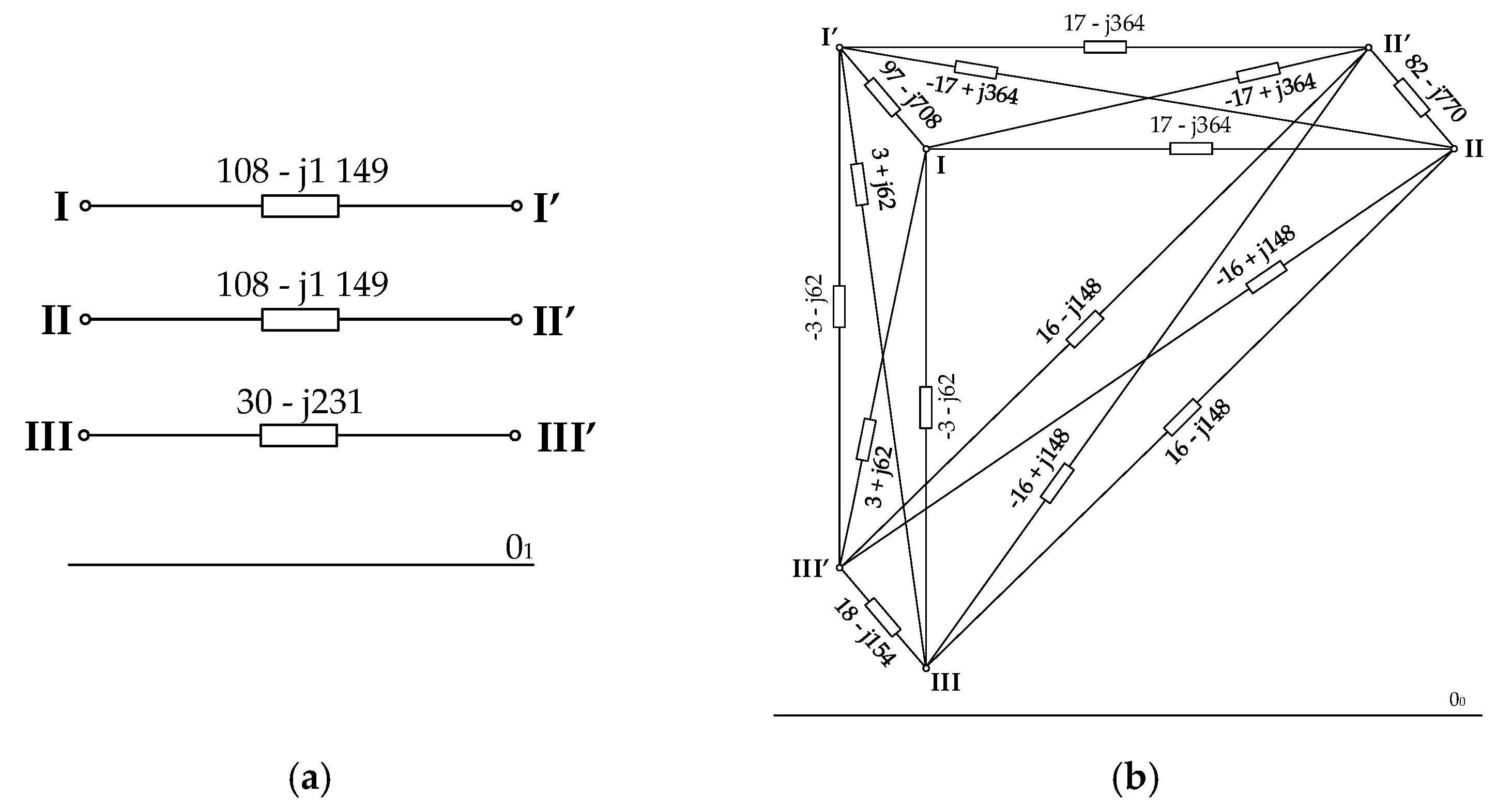
The equivalent schemes of a three-circuit, double-voltage transmission line (Table 2, Line 2) are presented in Figure 4. The symmetrical component’s series parameters and the admittance model Y_Spu for the positive-, negative- (Y_2pu = Y_1pu), and zero-sequence (Y_0pu) were determined using the previously described assumptions and procedure (Figure 3).

4.2. Analysis of Impedance Asymmetry

Obtaining full impedance symmetry requires making 9n single transpositions of phase conductors, where the term single transposition is understood as changing the position of two selected phase conductors of the line. Due to the conductor configuration in the line and the different voltage levels of the individual circuits, it is a technically and logistically complicated process. The cost aspect should also be considered because usually for lines with more circuits, the transposition of phase conductors requires an additional tower, which increases the costs of line construction. Thus, due to these drawbacks, line symmetrization by the transposition of its phase conductors is typically not pursued.

In the case of asymmetrical lines, in which the transposition of phase conductors is not applied, the admittance matrix of symmetrical components Y_S is a complete, full matrix. Supplying the line with a positive-sequence voltage and loading only with a positive-sequence current yields voltages of all symmetrical components (positive-, negative-, zero-sequences).

To determine the expected line impedance asymmetry and its effect on the transmission network’s ability to meet the quality requirements for the delivered electrical energy, the zero-sequence voltage values at the end of the unloaded circuit with the lowest rated voltage were determined. The analysis was performed for two actual three-circuit, double-voltage lines with various geometric asymmetries operating in the Polish system, i.e., Line 2 and Line 3. Asymmetric lines were supplied with symmetrical positive-sequence voltage in nodes I, II, and III and loaded with positive-sequence currents in nodes I’ and II’ with magnitudes equal to the long-term permissible current values of each circuit. The value of the zero-sequence voltage was determined as a function of the position of the extreme phases of Circuit III. The external conductors of Circuit III were moved symmetrically on both sides of the tower axis (Figure 5a) to determine the value of the zero-sequence voltage induced in this circuit per one kilometer of the line length (Figure 5b). The influence of earth conductors on the value of the zero-sequence voltage is noticeable. Over the entire range of changes, earth conductors reduce the value of the inducted zero-sequence voltage U₀.

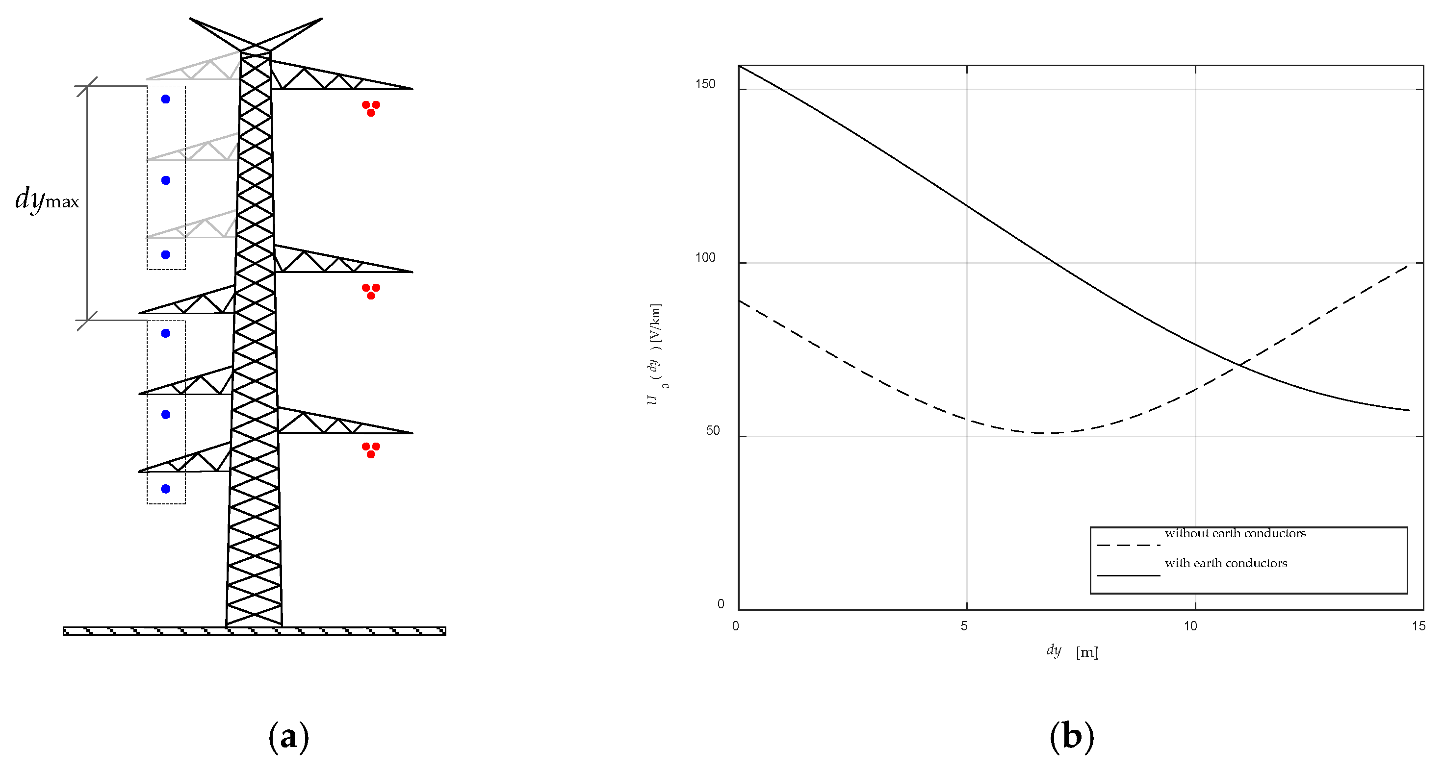
A similar analysis was performed for a double-circuit line with a vertical phase conductor configuration (Table 2, Circuit I and Circuit III of Line 3). The 110 kV voltage circuit position was continuously changed so that in extreme positions, this circuit was the lower (dy = dy_min = 0 m) and upper (dy = dy_max = 14.7 m) circuit of the real three-circuit line (Figure 6a), with dy denoting the absolute difference in the suspension height of the analyzed 110 kV circuit and Circuit II of Line 3 (Table 2). We noted a positive influence of earth conductors as they reduce the induced zero-sequence voltage as the lower circuit approaches the earth conductors (Figure 6b). In the extreme position (dy_max = 14.7 m), the voltage U₀ is reduced by about 100 V per one kilometer of the line length. The earth conductors have a beneficial effect on the top of the Line 3 circuit and an adverse effect on the bottom circuit.

For long asymmetrical lines, the zero-sequence voltage value may exceed the limit values. As a result, it tends to exceed the permissible values of voltage quality factors.

In addition, the analysis of individual impedance symmetrical components’ values for the symmetrical and asymmetrical transmission line model shows significant differences, which may impact the short-circuit impedance values calculated in systems with multi-circuit, multi-voltage lines. Such an analysis is presented in Section 5 of this paper.

4.3. Transmission Line Shunt Parameters

An overhead line’s capacitance is determined based on the charges on its conductors’ and these conductors’ potentials, using the mirror reflection method [18,19,20]. Similarly, as for the series parameters, the self and mutual parameters are calculated in the form of Maxwell’s potential coefficients by determining the ratio of the conductor potential to the density of the charge accumulated on it. These dependencies result from simple electrode systems (cylinder–cylinder) and are calculated based on geometric dimensions and material constants of conductors, resulting in the following:

$$P_{aa}=\frac{1}{2\mathsf{\pi }{\epsilon }_{0}l}\ln \frac{2h_a}{r_a}$$

(6)

$$P_{ab}=\frac{1}{2\mathsf{\pi }{\epsilon }_{0}l}\ln \frac{d_{ab’}}{d_{ab}}$$

(7)

where ε₀ is the electric constant permittivity of vacuum (in F/m); l is the length of conductor (in m); r_a is the radius of conductor a (in m); h_a is the suspension height of conductor a above the earth’s surface (in m); d_ab is the distance between conductor a and b; and d_ab’ is the distance of the conductor a from the mirror image of the conductor b. The potential coefficient P_aa applies to the given conductor a, while the coefficient P_ab corresponds to the pair of conductors a and b. As mentioned earlier, the inversion of the matrix of the transmission line’s potential coefficients P yields the capacitance of this line C.

The capacitance matrix C is an admittance type matrix. The off-diagonal elements of matrix C, taken with the opposite sign, are the capacitance values between the given phase conductor pair. The self-capacitance of conductor a is determined as the sum of the elements in row a of this matrix.

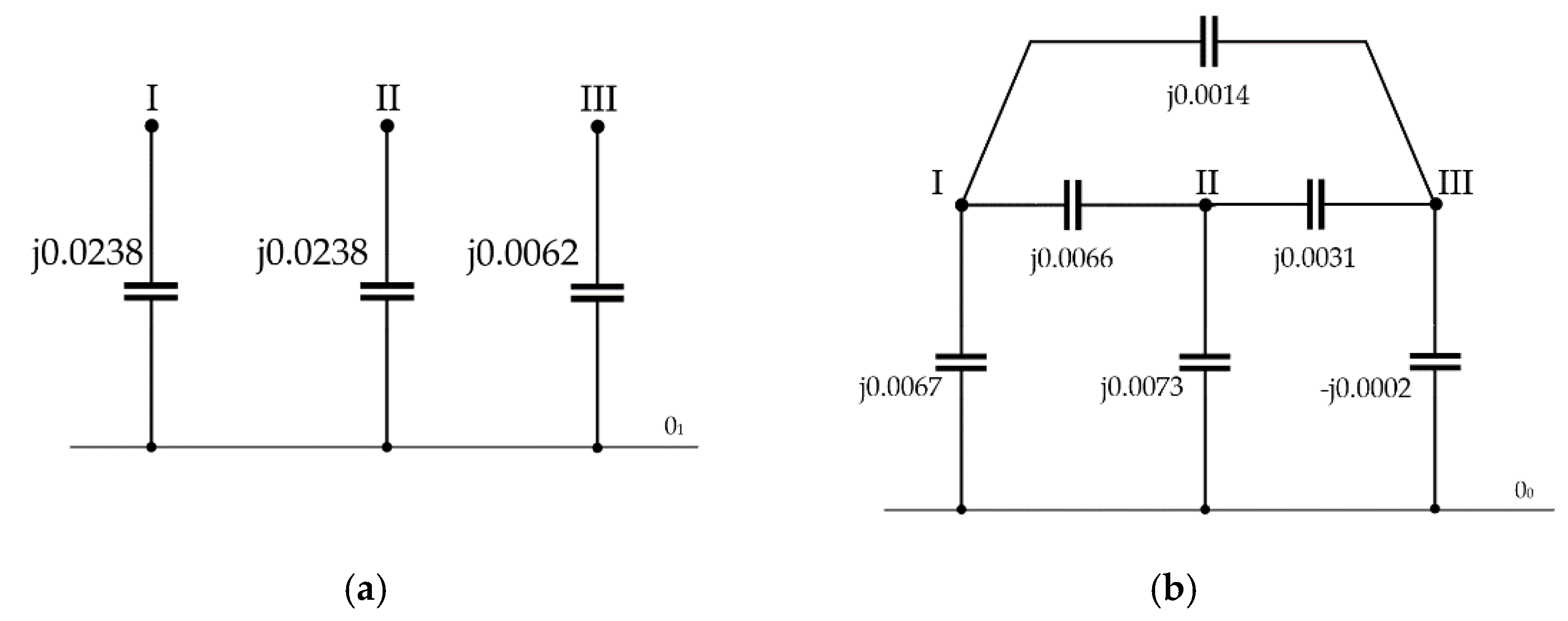
Similar to the series parameters, in Figure 7 we show the schemes of symmetrical component capacitances, namely the positive (C_1pu), negative (C_2pu = C_1pu), and zero-sequence (C_0pu) of the three-circuit, double-voltage transmission line (Table 2, Line 2).

4.4. Analysis of Capacitance Asymmetry

As with the series parameters, the lack of phase symmetrization of the line leads to capacitance asymmetry. In the transmission lines with different voltages’ ratings sharing the supporting structure, the line capacitance asymmetry is primarily noticeable for the lowest voltage networks. A similar situation was observed when there is a medium voltage line under the high voltage transmission line. Measurements and calculations presented in [22] show that the zero-sequence voltage in 15 kV lines could be on the order of several kilovolts. This condition significantly hinders the operation of the medium voltage line due to the inability to electrically ground it. For high voltage transmission lines, the appearance of additional voltage may affect the incorrect operation of earth-fault protection and may result in the appearance of significant zero-sequence currents under normal operating conditions of the network.

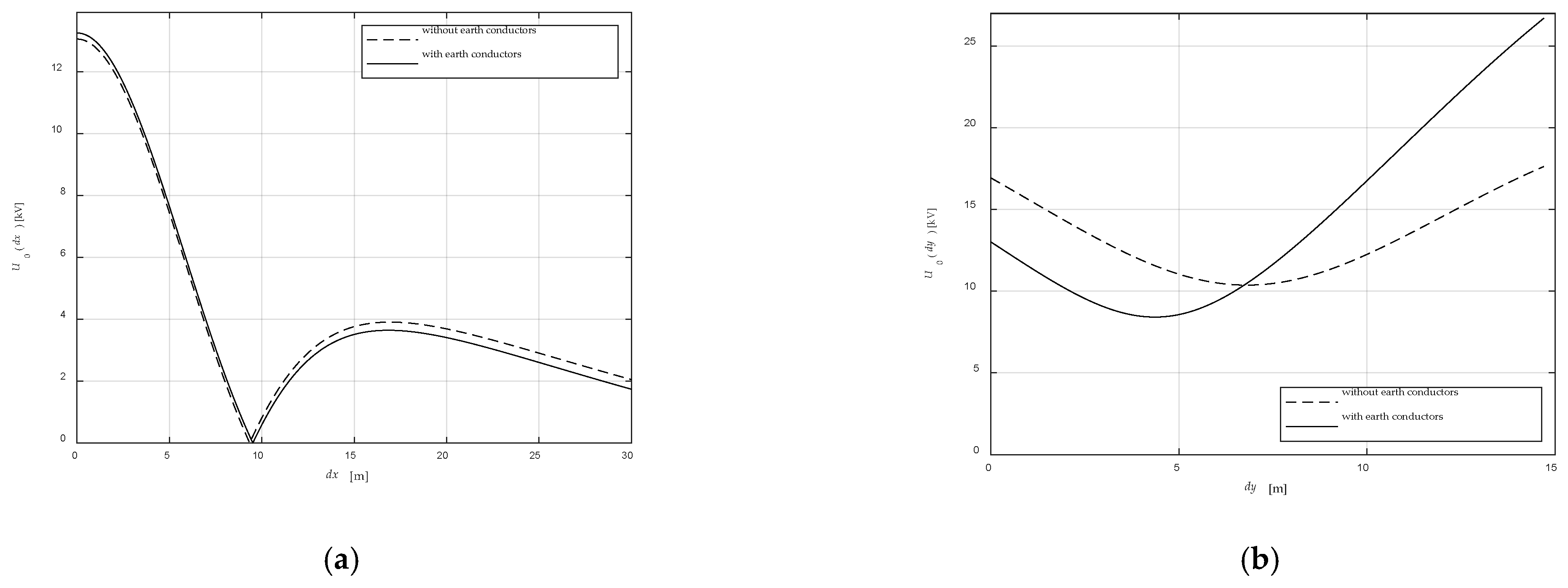
The capacitance asymmetry’s influence was determined by calculating the value of the zero-sequence voltage that appears in the lower voltage circuit when a higher voltage circuit is supplied. It should be emphasized that the zero-sequence voltage reduction effect will not occur in the case of transposition of the phase conductors in the circuit with a lower voltage. Here, the analysis was performed in the same way as the previous calculation of the series parameters for various conductors’ positions in the circuit. For Line 2, the lowest (i.e., closest to zero) that induced a zero-sequence voltage appears when the extreme phase conductors of Circuit III (i.e., L1, L3) are 9 m away from the tower axis (Figure 8a), which is realized in the real transmission line (Table 2).

In the case of Line 3, a favorable impact of earth conductors can be observed (Figure 8b). The earth conductors’ influence reduces the zero-sequence voltage in the range of changes dy = (0 ÷ 7) m. Further increasing the circuit (changes in the range dy = (7 ÷ 14.7) m) is characterized by a considerable influence of the earth conductors, causing an increase of the zero-sequence voltage value, in an extreme position, even by 10 kV.

5. Analysis of a Multi-Circuit, Multi-Voltage Transmission Line in the Power System

The consequence of the multi-circuit line’s lack of geometric symmetry is the phase asymmetry of individual circuits and the appearance of voltage and current asymmetry in the power system. With short lines, the differences between the symmetric and the exact model are not large; therefore, in such cases, the simplified symmetric models can be used. With longer lines, simplified symmetrical models may lead to significant errors when estimating the asymmetry factors for operating loads or the distribution of these currents in individual phases of the line circuits.

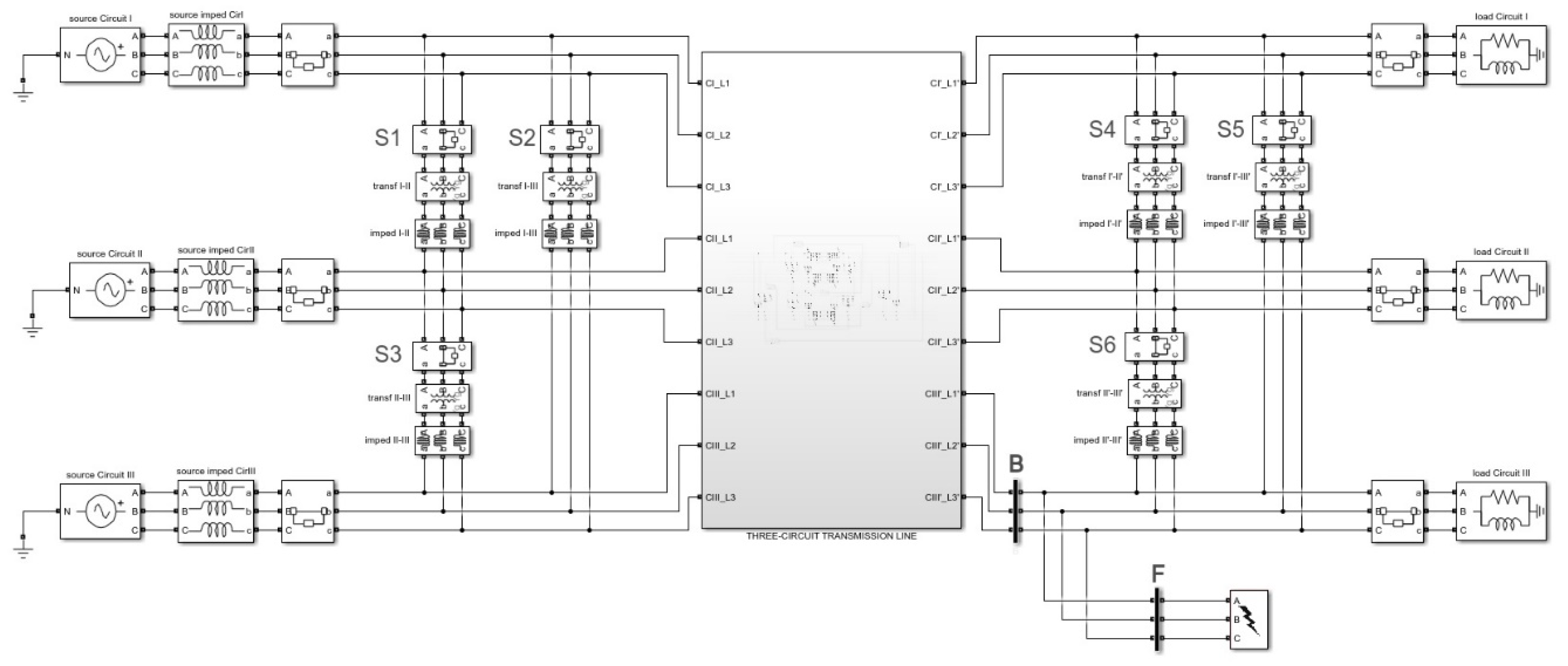
For simulation purposes, the MATLAB Simulink program was used to model a three-circuit line operating in a power system (Figure 9). The three-circuit transmission line’s model was realized using the basic R, L, C elements available in the Simulink library. Corresponding values were determined based on the line conductors’ geometric parameters and material constants, following the procedure described in Section 4 of this article. The external system was replaced with substitute sources from the line’s supply-side (nodes I, II, III) and from the other side (nodes I’, II’, III’) with loads of constant impedances.

Initially, the full equivalent of the external network was modeled. The full equivalent model includes the connections of all nodes of the transmission line [24,25]. The most adverse network operating conditions were determined by a preliminary testing of the model, which consisted of changing the values of the admittance parameters of connections between the selected transmission line nodes. The results made it possible to limit the external network model to a model containing only connections between the individual voltage levels at the beginning and ending nodes of the line (Figure 9), for which this effect was obtained. The parameters estimated using this simplified equivalent system were the indicators used to differentiate the performed analyses. In each case, we compared the voltages and currents in the system when the transmission line was symmetric and asymmetric. The line length was the main parameter of our analysis, which was performed for Lines 2 and 3 (Table 2).

5.1. Factors of Appearing Asymmetry with Symmetrical Supply and Load

The preliminary analysis of the influence that elements creating connections between individual circuits on the appearing voltage asymmetry showed is that the worst operating conditions of the system occur when the circuits are electrically far apart from each other. These conditions occur when there are vanishingly small (i.e., close to zero) admittances of connections at both ends of the line, which can be simulated by opening all switchers S1–S6 (Figure 9). Thus, further calculations were carried out for such parametrization. The calculations consisted of determining the voltages and currents at the ends of individual circuits, the symmetrical components of these quantities, factor α₀ (the zero-sequence voltage module ratio to its positive-sequence), and factor α₂ (the negative-sequence voltage module ratio to its positive-sequence). The factors for currents were defined analogously. Due to the symmetry of the loads, they are numerically identical to the corresponding voltage factors.

For Line 3 (the line with greater geometric asymmetry), calculations were made for four cases: a load of Circuit I (400 kV) and Circuit II (110 kV), a load of Circuit I and Circuit III (110 kV), a load of all circuits carrying the maximum long-term permissible currents, and half of these currents. For the 400 kV circuit, the long-term permissible current was 2850 A, and for the 110 kV circuits, 730 A. The purpose of considering the first two cases was to determine which of the 110 kV lines is more exposed to voltage asymmetry. The results presented in Figure 10 clearly confirm that the lower line (Circuit III) is more exposed to voltage asymmetry. In both these cases (the load on Circuits I and II, and Circuits I and III), the highest asymmetry factors appear in Circuit III. National regulations, according to [26], give only limit values of the α₂ factor, which should not exceed 2%. In the analysis of the diagram given in Figure 10b, it should be stated that this limit value is achieved for a line with a length of about 25 km with a full load of Circuits I and III and the open-circuit operation of Circuit II. Additionally, it should be noted that the values of α₀ factors are relatively high, reaching several percentage points already at such lengths. This will result in high zero-sequence currents that may adversely impact the earth-fault protection and safe operation of the system.

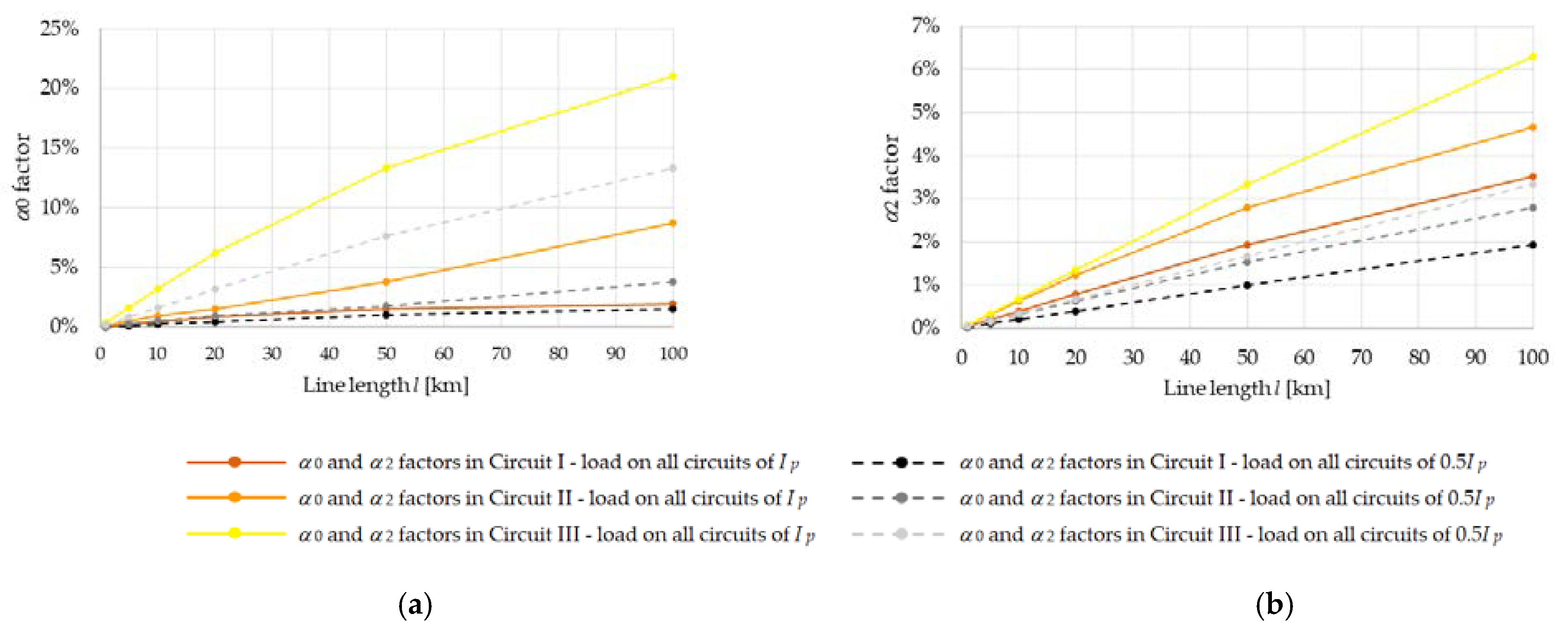
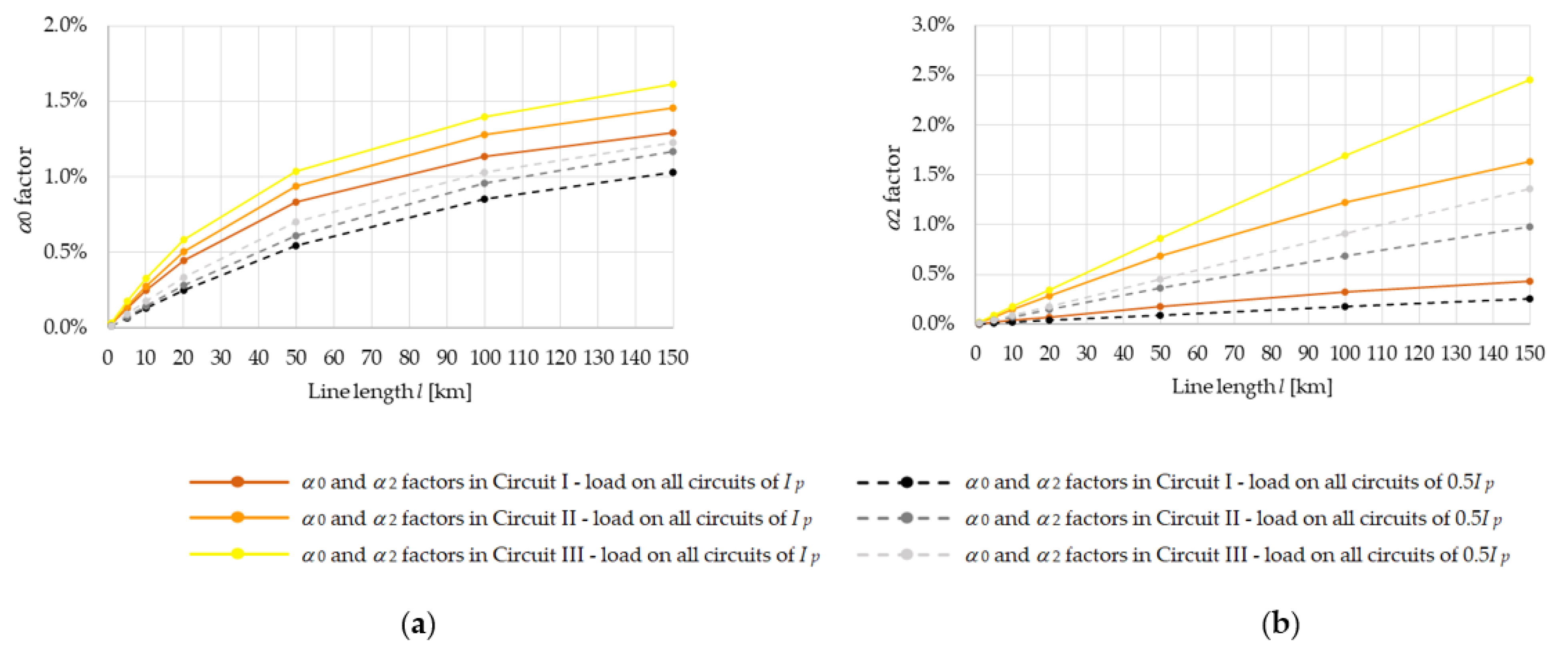
Figure 11 shows the α₀ and α₂ factors for all circuits’ load with the full and half values of the long-term permissible currents. The circuits’ loading with half of the maximum long-term permissible currents is closer to the actual loads occurring in the power system’s operation. In this case, the α₂ factor reaches the limit at 30 km of the line length for the full load and 60 km for the reduced load (Figure 11b). However, even with a reduced load, the α₀ factor values reach 5% and 8%, respectively (Figure 11a). Much lower values are achieved by the factors for Circuit I with a 400 kV voltage. These results confirm the necessity to perform transpositions on such lines. In this case, due to the relatively small distances between the phases of Circuits II and III (110 kV), it is technically possible to transpose these circuits, e.g., using a triangular conductor configuration on transposition towers.

Due to the smaller geometric asymmetry and the estimated zero-sequence voltage results presented in Section 4 of the article, analyses were performed for Line 2, assuming a load of all circuits with their full and half maximum long-term permissible currents. For Circuits I and II (400 kV), the long-term permissible current was assumed as for Line 3, while for Circuit III (220 kV), the current was 1220 A. Figure 12 shows the α₀ and α₂ factors in function of the line length.

For the analysis of Line 2, no significant values of both α₀ and α₂ factors were observed. Even for a 120 km long line, the limit value of these factors is not reached.

5.2. Quantitative Comparison of Short-Circuit Currents for Symmetrical and Asymmetrical Models

Using the system’s model developed in this work, an analysis of the influence of the line asymmetry on short-circuit currents was also performed. In this case, three-phase and single-phase-to-earth faults at the end of Circuit III were modeled, as shown in Figure 9. As in the asymmetry analysis, for short-circuit studies, the systems for which the differences between the symmetric and asymmetric models are the greatest were determined. In this case, these are systems in which the ends of the individual circuit are electrically close to each other, which were realized by connecting a transformer between the ends of circuits with different voltages and couplings between circuits with the same voltage; such operation of circuits is reffered to as “close”. Three system configurations described in

Table 5. The short-circuit current changes indexes for Line 3 depending on the individual lines’ connection system’s ends.

Case Studied	Line Length	Relative Circuit III Current Index in Point B (Figure 9) during Fault		Relative Short-Circuit Current Index in Point F (Figure 9)
		Three-Phase Fault	Single-Phase- to-Earth Fault	Three-Phase Fault	Single-Phase- to-Earth Fault
	km	%	%	%	%
Circuits I and III are “close” and Circuits II and III are “close”	10	6.02	3.91	2.23	2.72
	100	12.41	13.71	2.17	2.58
Circuits I and III are “close”	10	3.51	1.07	2.00	0.92
	100	4.17	2.33	1.86	1.41
Circuits II and III are “close”	10	5.37	2.25	3.43	3.65
	100	8.16	2.53	5.07	4.64

were analyzed, where the “close” operation of analyzed circuits was simulated by closing the corresponding switchers S1–S6 (Figure 9). For example, in the case where Circuits II and III are electrically “close” to each other, the switcher S6 is closed (Table 5). In such cases, short-circuit current components, i.e., high-value currents, flow through all circuits, and their interaction with each other is noticeable. Here, the analysis parameter was also the short-circuit power of the power supply systems. The basic values of short-circuit power were adopted for 400, 220, and 110 kV, respectively: S_Q400 = 27.7 GV∙A, S_Q220 = 15.2 GV∙A, S_Q110 = 7.6 GV∙A. With an asymmetric model, the currents of single-phase-to-earth faults at a given location are different for each phase. For three-phase faults, the same currents do not flow in individual phases.

For comparative purposes, the change of the short-circuit current index I_% was determined:

$$I_{\%}=\frac{I_{\mathrm{as}}-I_{\mathrm{s}}}{I_{\mathrm{s}}}\cdot 100\%$$

(8)

where I_as is the maximum value of the phase current (for a single-phase-to-earth fault, I_as is the phase short-circuit current giving the highest value; for a three-phase fault, I_as is the highest current in the phase) at the fault location or in the tested line circuit for asymmetrical line model; and I_s is the phase current value at the fault location or in the tested line circuit for symmetrical line model.

Table 5 shows the values of the current change indexes for two line lengths (10 km and 100 km) with various arrangements of Line 3’s ends operation for the basic values of the short-circuit power sources connected to the beginning of each line circuits.

The differences in the short-circuit currents are relatively small, reaching a maximum of about 5% for a 100 km line. More considerable differences were observed in the shares of these currents flowing through Circuit III phases, which reach over 13% for the long line with a single-phase-to-earth fault.

Another analysis was carried out to determine the impact of short-circuit powers on the differences of short-circuit currents (

Table 6. Indexes of changes in short-circuit currents for Line 3 depending on the short-circuit power of the sources supplying individual circuits (S_Qx = 1 means the basic short-circuit power).

Relative Short-Circuit Powers of the Systems	Line Length	Relative Circuit III Current Index in Point B (Figure 9) during Fault		Relative Short-Circuit Current Index in Point F (Figure 9)
		Three-Phase Fault	Single-Phase- to-Earth Fault	Three-Phase Fault	Single-Phase- to-Earth Fault
	km	%	%	%	%
SQ400 = 1	10	6.02	3.91	2.23	2.72
SQ110 = 1	100	12.41	13.71	2.17	2.58
SQ400 = 1	10	5.47	3.56	1.50	2.33
SQ110 = 0.5	100	12.28	13.57	2.09	2.57
SQ400 = 0.5	10	5.99	3.83	2.28	2.75
SQ110 = 1	100	12.24	13.28	2.15	2.56
SQ400 = 0.5	10	5.43	3.49	1.54	2.36
SQ110 = 0.5	100	12.11	13.14	2.06	2.55

). The practical conclusion from these considerations is that the percentage currents differences depend only slightly on the short-circuit power value, both in the short-circuit currents and in their branch shares.

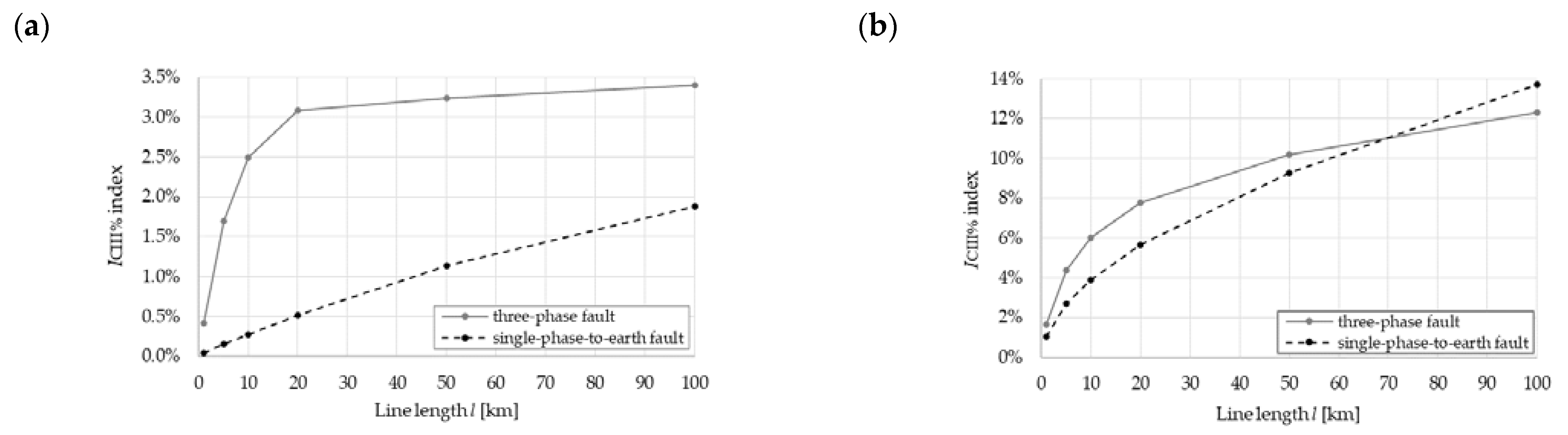
Figure 13 shows the branch’s current indexes’ dependence for Line 2 and Line 3 (in Circuit III) in the function of the line length for a single-phase-to-earth and three-phase faults in the most unfavorable system operation condition, i.e., in the system where Circuits I and II are “close” to Circuit II at their ends. In this case, a clear relation of the index I_% with the line length was observed. For three-phase faults, the indexes’ values begin to stabilize and level off with increasing length, while the single-phase-to-earth faults curves continue to increase.

6. Summary and Conclusions

The increased demands for electrical energy, the development of a generation of unstable energy production, and continuous efforts to improve power supply reliability make it necessary to expand the transmission system. On the other hand, environmental constraints make it challenging to build and operate new transmission lines. A certain compromise between these opposing interests is the construction of multi-circuit lines, especially multi-voltage ones. In terms of the occupied area’s width for the construction of overhead lines and the electromagnetic field strength in the line’s vicinity, this solution is very beneficial, which we have shown in Section 1 and Section 3. However, there are also new problems in the design and modeling of such elements. The article focused on two issues, i.e., line design from the mechanical (i.e., selection of the optimal span length) and electrical (i.e., an analysis of the effect asymmetry has on the electrical parameters of the line, namely, the impedance and capacitance) point of view. The asymmetry of transmission line electrical parameters affects the operation of the entire line electrical environment and the accurate determination of the characteristic short-circuit currents associated with the selection of conductors, as well as the operation of the transmission line protection automatics.

The analysis we performed shows that, from the mechanical point of view, for shared transmission line construction with different voltage ratings, primarily when a 110 kV circuit is carried with 400 and/or 220 kV lines, there may be some difficulties with the coordination of stresses and sags, but a compromise is possible in this case. The problem practically does not occur when all circuits are made of similar conductor types (as in the 400 and 220 kV lines).

In terms of the phases of its individual circuits, a multi-circuit line is an asymmetric element that can be symmetrized by the conductor transposition of the individual line circuits. However, this is a complicated procedure to implement, in which it would sometimes be necessary to place an additional tower next to the main path of the line. The asymmetrical structure results in the asymmetry of the electrical parameters of the line. Analyzing the transmission line impedances and capacitances separately, we focused on showing the effect of the zero-sequence voltage appearing in the unsupplied circuit under the influence of symmetrical voltage in other circuits (capacitance asymmetry, as seen in Figure 8) and the influence of the zero-sequence voltage appearing in the supplied but unloaded circuit under the influence of symmetrical loading of other circuits (impedance asymmetry, as seen in Figure 5b and Figure 6b). The influence of the zero-sequence voltage is especially visible in the circuits with the lowest rated voltage. It is different for various line geometries, and hence a conclusion on the certain possibilities of optimizing the circuits’ position in relation to each other was derived.

The second computational aspect of the article was the estimation of the voltage quality factors α₀ and α₂ that may appear during the operation of the asymmetrical multi-circuit lines in the power system, as well as errors in the estimates of short-circuit currents when using a symmetrical model instead of an exact asymmetrical one. The analyses carried out on two types of three-circuit lines with small (Line 2) and large (Line 3) geometric asymmetry show that for Line 3, both the asymmetry factors and the current indexes, even for short sections of such lines (several kilometers), can be significant and can affect the correct operation of the entire system. The symmetrical model can be used for lines with small geometric asymmetry, even for relatively long lines (of several dozen kilometers). It follows that for specific objects, such as multi-circuit, multi-voltage lines, the electric models of these lines should be determined as exact, and only in exceptional cases can simplified symmetrical models be adopted. It is also necessary to use conductor transposition, especially in the case of carrying 400 and 110 kV circuits on a shared structure [27], which is possible using appropriate towers.