A Case Study of a Virtual Power Plant (VPP) as a Data Acquisition Tool for PV Energy Forecasting

Abstract

This article describes problems related to the operation of a virtual micro power plant at the Faculty of Electrical Engineering (FEE), Czestochowa University of Technology (CUT). In the era of dynamic development of renewable energy sources, it is necessary to create alternative electricity management systems for existing power systems, including power transmission and distribution systems. Virtual power plants (VPPs) are such an alternative. So far, there has been no unified standard for a VPP operation. The article presents components that make up the VPP at the FEE and describes their physical and logical structure. The presented solution is a combination of several units operating in the internal power grid of the FEE, i.e., wind turbines, energy storage (ES), photovoltaic panels (PV) and car charging stations. Their operation is coordinated by a common control system. One of the research goals described in the article is to optimize the operation of these components to minimize consumption of the electric energy from the external supply network. An analysis of data from the VPP management system was carried out to create mathematical models for prediction of the consumed power and the power produced by the PVs. These models allowed us to achieve the assumed objective. The article also presents the VPP data processing results in terms of detecting outliers and missing values. In addition to the issues discussed above, the authors also proposed to apply the Prophet model for short-term forecasting of the PV farm electricity production. It is a statistical model that has so far been used for social and business research. The authors implemented it effectively for technical analysis purposes. It was shown that the results of the PV energy production forecasting using the Prophet model are acceptable despite occurrences of missing data in the investigated time series.

1. Introduction

The European Green Deal presented by the European Commission on 11 December 2019 assumes that by 2050, the EU will become “the first climate neutral continent”. This goal requires achieving zero net greenhouse gas emissions and breaking the interdependence of economic development with the consumption of natural resources. In this regard, it is assumed that EU countries will achieve zero net emissions in particular by reduction of existing emissions, investments in green technologies and environmental protection [1]. These assumptions will also result in more dynamic development of the renewable energy market and its greater share in the total power generation.

According to the Central Statistical Office in Poland [2], the energy obtained from renewable energy sources (RES) comes mainly from solid biofuels (65.56%), wind farms (13.72%) and liquid biofuels (10.36%). The total primary energy obtained from renewable energy sources in Poland in 2019 was 396,498 TJ. The gross final consumption of energy from renewable sources has increased in recent years by 8.8%, from 325,387 TJ in 2015 to 376,060 TJ in 2019. The increasing share of renewable energy sources in the power system, especially weather-dependent sources (wind, PV), may cause various complications in the operation of the power system, but may also support its operation in special emergency conditions. One possible solution in this case is virtual power plants. A virtual power plant (VPP) is a combination of decentralized units whose operation for the power grid is coordinated by a common control system. These units can be electricity producers such as biogas, wind and photovoltaic energy conversion systems, cogeneration hydroelectric power plants, electricity consumers, electricity storage facilities and other.

The goal of a VPP is joint marketing of electricity and flexibility for the entire group of interconnected energy producing devices. Any decentralized entity producing, storing or consuming electricity can become a part of a VPP. Unlike traditional power plants, VPPs do not own energy resources. Instead, they own the data that is transferred between each resource on the grid. VPPs focus on optimizing the way each resource is connected to the grid, and thanks to the flexibility of a decentralized grid, they can effectively balance the grid. The VPPs are able to maintain this balance by combining in their portfolio different energy sources—such as solar, wind, biogas, water energy and more. Because there are no uniform standards for power systems, there are various models of VPPs as well as of grids they support. Some of them focus on the grid reliability, while other models focus on maximizing economic benefits by selling surplus energy services to larger grids [3,4]. By fast adjustment to the amount of electricity available in the grid, their aggregate capacity allows them to optimally track the electricity price on the electricity exchange [5,6], and thus to offer their electricity to the market in an effective way. In [7], the authors describe the tender strategy of a VPP on the common energy and reserve market, while [8] deals with the tender strategy of an electric vehicle aggregator that participates in both day-ahead and reserve energy markets. In [9], a model is presented that also includes the grid thermal loads and the energy storage. Another critical aspect of large-scale RES integration is the operational security of the VPP operated network. In [10], the authors describe a case of a VPP containing hydropower plants (HPP) and energy storage systems (ESS). They analyze in detail power quality (PQ) issues on the basis of a set of 26-week multi-point, synchronous measurements of power quality levels at four related points. The most important conclusion from these studies is that the overall VPP impact on the long-term grid performance in terms of the PQ was positive. In the works [11,12], the authors discuss problems of grid security in terms of the voltage regulation and due to excessive grid frequency. Adding distributed generation (DG) to the VPP paradigm allows for consistent central control and coordinated market integration of several widely distributed energy sources. As a consequence, the VPPs can participate in the frequency control by regulating their output power in a coordinated manner for the sake of system stability. Another important problem discussed in [13,14] is the uncertainty of energy production from the RESs. The uncertainty and inaccuracy of forecasts increases with the time horizon and has a significant impact on a VPP energy management planning. This paper focuses on the problem of predicting electricity obtained from photovoltaic sources operating as one of the elements of a virtual power plant (VPP). A new prediction algorithm, which has not been used for these purposes so far, has been implemented.

2. Materials and Methods

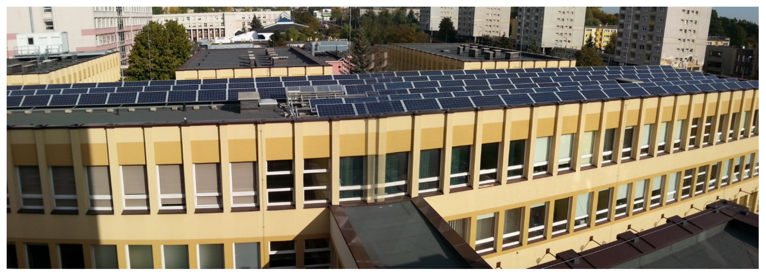
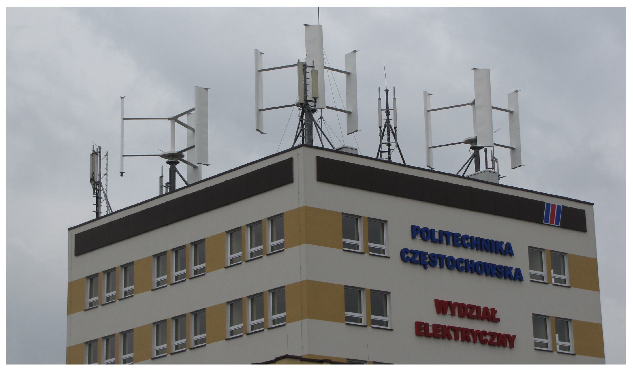
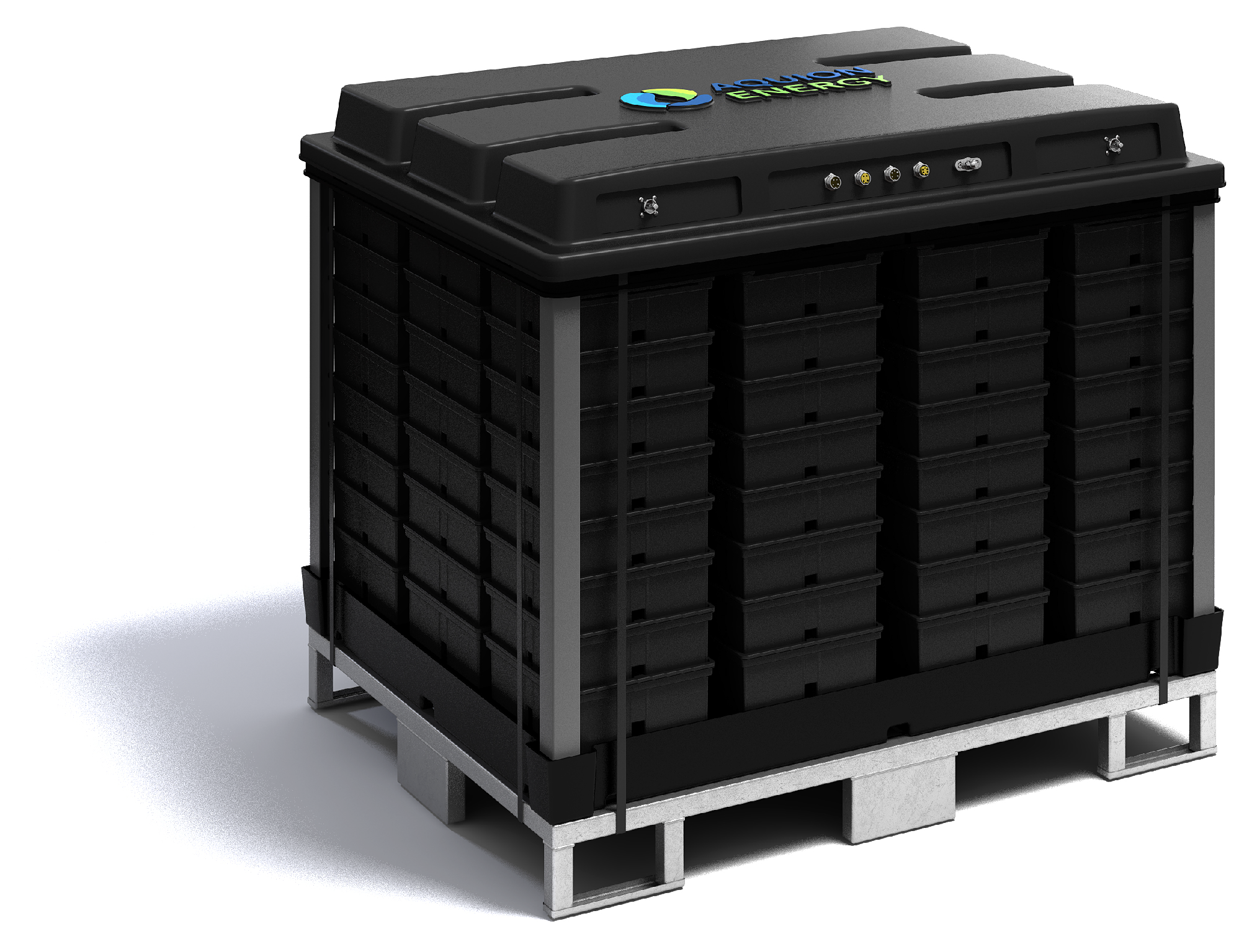
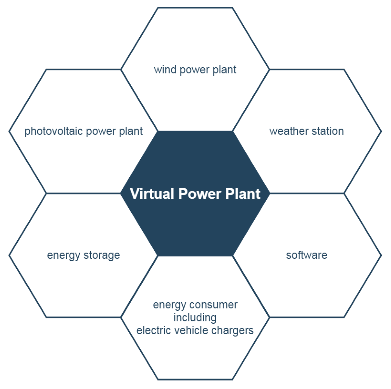
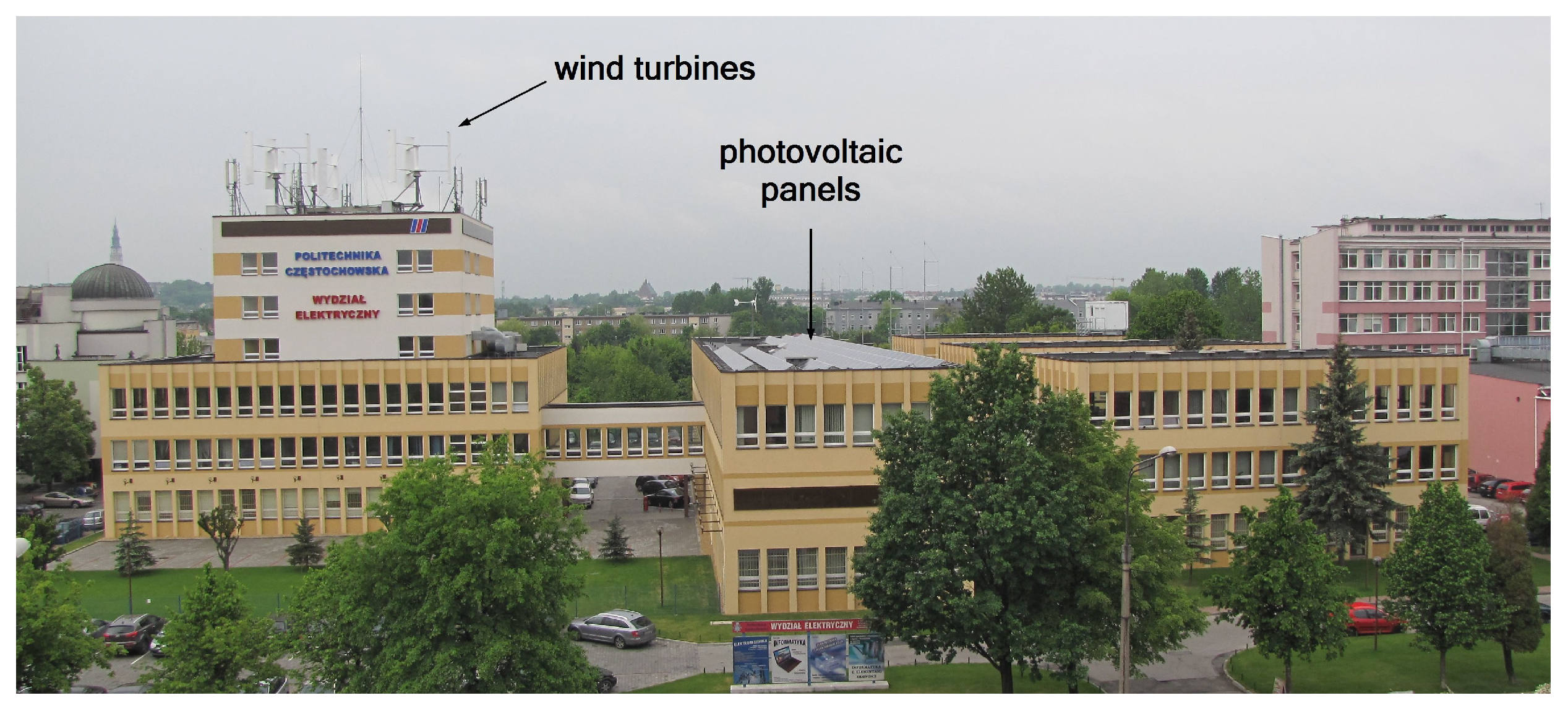
2.1. VPP Hardware Infrastructure

The importance of renewable energy sources is increasing year by year. Stochastic and intermittent nature of energy production from these sources negatively affects stability of power systems. A solution to this problem may be integration of distributed sources that would enable aggregation of production capacities as well as energy storage capacities. As a result, optimal energy management would become possible [15,16]. The idea of VPP can also support solutions in the Demand-Side Management (DSM) programs [17]. The virtual micro-power plant operating at the Faculty of Electrical Engineering (FEE), CUT, is a system that was developed gradually by adding new hardware and software components. Initially, from the point of view of the power system, the FEE buildings were only an electricity consumer. Renewable energy conversion systems, i.e., photovoltaic panels and three vertical axis wind turbines, were installed at the first stage to convert energy from the sun and wind into electricity. Next, the system was enriched with an energy storage. The final stage (so far) was building three charging stations for electric cars, which increased the demand side of the system. Simultaneously with the hardware development, the IT software structure was developed so that it became possible to monitor and manage not only the virtual power plant as a whole, but also its individual elements. The components making the virtual micro-power plant are shown in Figure 1.

Nowadays, the challenge is to design and build a photovoltaic power plant to achieve high benefits at low cost. Individual components of the power plant are examined and selected, and then the number of particular components and their distribution are specified [18,19]. There are created innovative management systems [20,21,22]. Photovoltaic power plants are becoming parts of larger systems that can store the produced electric energy [23]. Mobile power plants are designed to ensure fast charging of hybrid and electric cars [24]. Similar problems also apply to wind farms [25,26,27,28].

In the case of the micro VPP located at the FEE, the design of renewable energy conversion systems was motivated mainly by three factors: (1) reduction of the negative environmental impact by decreasing the consumption of electricity from conventional power plants, (2) development and practical testing of solutions related to the construction of a virtual power plant and analysis of the obtained solutions from the scientific perspective, (3) reduction of incurred costs. The construction of the wind farm and the photovoltaic plant began at the same time. Due to the shape and location of the FEE buildings, it was decided to place photovoltaic panels and wind turbines on the flat roofs of two buildings. The wind turbines were located at the highest possible place, while the photovoltaic panels were installed on the roof of the lower building. The location of the renewable energy conversion systems is shown in Figure 2.

The power of the photovoltaic power plant, shown in Figure 3, is 33 kWp. It consists of 132 polycrystalline panels with a power of 250 Wp each. A single panel size is 1640 × 990 × 40 mm and it weighs 19 kg. The efficiency of a panel is 15.6%. The photovoltaic panels are connected to two three-phase inverters from GoodWe, 17 kW of nominal power each. They can operate with 20% overload. Due to the panel distribution geometry, most of the panels (19.00 kWp of power) are connected to inverter #1, the remaining panels (14.00 kWp of power) are connected to inverter #2. The output circuit of inverter #1 is connected to three single-phase Victron Energy inverters, which include microprocessor-based battery charging controllers. They make it possible to control the flow of electricity coming from the photovoltaic power plant. By means of established control rules, this energy is directed either directly to the current consumption of the FEE facilities or to the energy storage. The system is configured so that the charging of the energy storage can be carried out only from part of the power plant, i.e., the energy passing through inverter #1. The energy passing through inverter #2 is transferred to the city power grid. This configuration results from the limited storage capacity (25 kWh) and from the analysis of the FEE facilities needs. The installation brings a measurable ecological, economic and scientific effect. In particular, research on energy quality is carried out, see, e.g., the results presented in [29].

The wind power plant, which can produce 30 kW of total power, consists of three H-Darrieus-type 10 kW turbines with a vertical axis of rotation, is shown in Figure 4. Each turbine is equipped with a direct drive permanent magnet synchronous, low-speed, coreless generator (38 pairs of poles) and connected to the power grid via an inverter. The turbines can start to operate at wind speeds above 1.5 $\frac{m}{s}$ (low cut-in wind speed). They achieve high efficiency, up to 95% of the captured aerodynamic power, at 150 rpm. The maximum (nominal) power is achieved at the wind speed of 12 $\frac{m}{s}$. The safety system stops the turbine is if the wind speed exceeds 17 $\frac{m}{s}$ (cut-out wind speed).

The installation of renewable energy conversion systems had a positive effect on the energy balance of the FEE buildings. Due to the production of electricity from own sources, the volume of energy drawn from the power system was reduced. In general, the share of electricity generated from renewable energy sources in Poland is less than 14%. Therefore, any initiative that increases this share results in decrease of ${\mathrm{CO}}_2$ emissions, as the amount of energy produced from burning fossil fuels is reduced. In addition, consumption of the energy produced on site reduces the load on the power grid and the losses associated with the transmission of electricity. The next stage of the virtual micro power plant development was installation of an energy storage. It made it possible to control the generated electricity stream so as to consume as much energy produced on site as possible. The energy storage allows us to minimize the transfer of the generated energy to the power grid. The installed energy storage is a battery based on the innovative AHI (Aqueous Hybrid Ion) technology. The battery is made of stainless steel and synthetic cotton is used as a separator. The anode is made of carbon composite, the cathode material is manganese oxide, and the electrolyte equivalent is salt water (electrolyte sodium sulphate). The whole battery is closed in a plastic housing. A great advantage of this solution is that there is no risk of explosion, hence there is no need to prepare a special room for the battery placement. This type of energy storage can be installed in places with more stringent environmental protection requirements, in offices or in private homes where people or animals are present. The unit used in the FEE micro VPP is the M110-LS83 battery with capacity of 25 kWh at 48 V. The M series battery consists of twelve S series batteries connected in parallel. It is possible to connect to the battery a dedicated monitoring system (BMS), that allows to measure the level of charge, current, voltage or temperature. The M series battery is shown in Figure 5.

The Vantage Pro 2 Plus weather station from Davis Instruments is a complementary element of the VPP. It makes it possible to conduct various types of the VPP-related analyzes and scientific research. The weather station unit is located next to the wind farm and the photovoltaic plant. Thanks to the recorded weather data and the information on the volume of electricity produced from the renewable energy sources, it is possible to find relationships between them. The weather station allows for continuous measurement of such quantities as: temperature, humidity, pressure, precipitation, wind speed and direction, and solar radiation including the UV radiation. Data update period takes from a few to 60 s depending on the measured quantity. It can therefore be assumed that successive sets of weather data are recorded with a 60 s interval.

Another element that was added to the FEE micro VPP were three Ecotap WG2 car chargers. These chargers enable three-phase charging of electric and hybrid plug-in vehicles. The chargers are equipped with type 2 sockets and each charger can charge two vehicles simultaneously. The charging power is adjusted individually to each vehicle being charged. Initially, the chargers were used to a small extent, but the number of cars using this charging option has been increasing every month. After the several years of the FEE VPP operation we can state that the installation contributes to reduction of ${\mathrm{CO}}_2$ emissions and supports popularization of ecological solutions. Almost all the produced electricity is consumed locally. Due to relatively low power of the generation sources, the produced power is usually lower than the FEE demand, so situations when the produced electricity is fed into the power grid are exceptional. Several electricity meters were installed in the FEE buildings to enable monitoring of the electricity consumption in individual pavilions. A few years ago, one pavilion was completely rebuilt, and electricity meters were installed on each floor of the pavilion. Since then, it is the best of all the metered pavilion in terms of electricity consumption. The meters can measure active and reactive energy, both drawn from and fed to the grid. Additionally, it is possible to measure instantaneous values of active and reactive power, voltage, current and frequency.

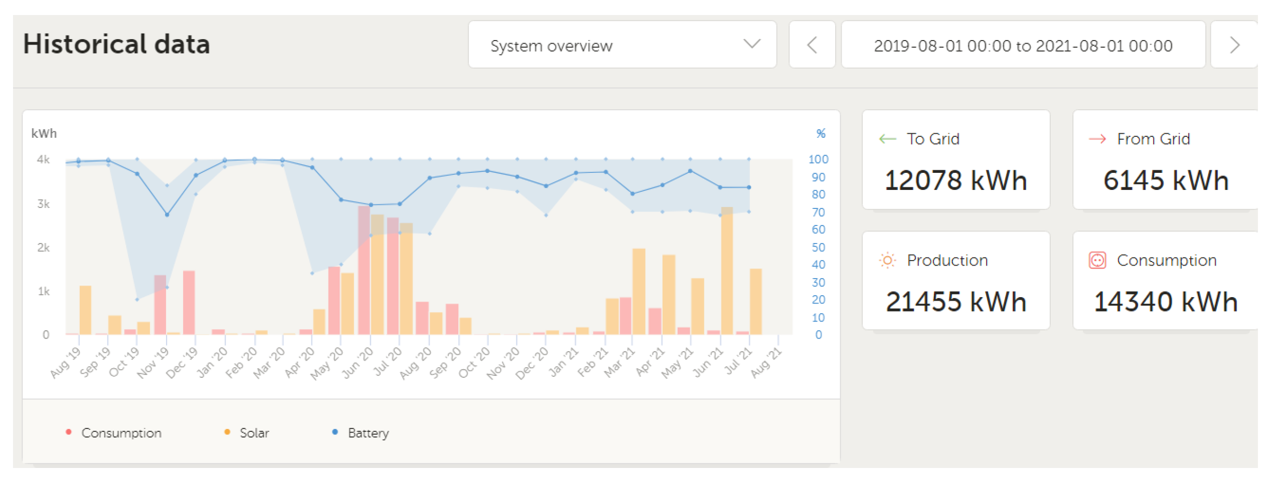
2.2. VPP Software Infrastructure

Each component of the VPP physical infrastructure can communicate with other components and transmit measurement data. Some components have dedicated software that enables monitoring and, in the case of the energy storage, also control of the charging and discharging process. The photovoltaic power plant and the energy storage are supervised by three single-phase Victron Energy MultiPlus 48/5000/70 inverters. Monitoring and management of energy flows is carried out by the software supplied with the inverters. This system is locally monitored and controlled through the Color Control GX panel. Remote access to the installation is possible through the Victron Remote Mangement (VRM) software. On PC computers, the access can be obtained through a web browser (address https://vrm.victronenergy.com/login) (accessed on 3 August 2021), on mobile devices through a dedicated application. Figure 6 shows the basic block diagram view of the system. The main element of this part of the system, which monitors and controls the power flows, is the element marked in blue (Victron Energy Inverters).

The photovoltaic power plant, denoted as PV Inverter in Figure 6, as well as elements denoted as Grid and AC Loads, which represent outputs from the inverters, are connected to the system. The inverters have two types of outputs: guaranteed and non-guaranteed. The difference between them is that if the power supply is disconnected from the power grid and, at the same time, the electric energy is generated by the photovoltaic power plant or is drawn from the energy storage, the voltage at the corresponding guaranteed output is maintained and connected loads are still powered. A guaranteed output works like a classic UPS. In the same case, the inverter cuts off the voltage at an non-guaranteed output. If electric energy was supplied to the loads through a guaranteed output, in emergency situations, such as fire in a building, people could get an electric shock despite disconnecting the FEE installation from the power grid. Due to those safety reasons, the energy produced by the photovoltaic power plant or stored in the energy storage is supplied to local loads in the FEE buildings through the non-guaranteed output denoted as Grid in Figure 6. A negative value on this block indicates that energy flows from the PV plant or the storage facility to the consumers. Only the subsystem that controls the energy storage is supplied through the guaranteed output denoted in Figure 6 as AC Loads. It is a small part of the installation located by the energy storage that requires non-stop power supply. Lack of power necessitates a manual restart of the subsystem. The energy to the AC Load output is directed first from the PV power plant, later from the energy storage. If there is no energy available from these sources, it is drawn from the building infrastructure (external power grid). In such case, this part of the micro VPP becomes an electricity consumer and the flow value on the Grid block becomes positive. The final component of the system is the energy storage. The application allows for tracking its level of charge, voltage, current and its current status, i.e., charging, idle or discharging. In the case of other components, we can track the instantaneous power on individual phases (L1, L2, L3) and the total three-phase power. The application main screen also displays the real time animation of how the electric energy is flowing between individual VPP components. At the same time, it is possible to view historical data on the production of energy by the PV installation, the energy consumption and the storage charge level, including the maximum and minimum values of charge over a specified period. Additionally, for a given period, we can get a summary of how much energy was produced, how much energy was consumed through the guaranteed output, and how much was drawn and returned through the non-guaranteed output. The minimum time range that can be presented on the chart is one hour (in this case, the values are aggregated to fifteen-minute periods), the maximum time range is two years (in this case, the individual values are aggregated on a monthly basis). The database contains historical data on the electricity production and consumption from the last five years. A chart presenting the basic historical data from the last two years is presented in Figure 7. The blue plot shows the average monthly level of the energy storage charge, the light blue area represents the maximum and minimum values in a given period. These values are scaled in percent—the right scale of the chart. The aggregated monthly energy production and consumption in kWh are presented as orange and pink bars, respectively. The decrease of the energy consumption from May 2021 (in comparison with the same period of year 2020) is related with physical reconfiguration of the load connection structure, i.e., supply of energy through the guaranteed and the non-guaranteed outputs as described above, which took place just in May 2021.

It is also possible to check what the electric energy was used for, i.e., loading the storage battery, direct consumption (guaranteed output) or consumption by loads in the FEE buildings (non-guaranteed output). This information is presented as in Figure 8. In addition, the percentage division of energy in the last periods is shown, starting from the last day and ending with the last year.

Another option is to observe where the electricity transferred through the guaranteed output was drawn from. Figure 9 shows the breakdown of the consumed electricity by the source of origin.

A user can define more ways of how different historical data are presented. The number of observed quantities can be freely configured depending on the needs. Ready-made widgets that can be added to the dashboard are used for this purpose. The only thing that needs to be done is to specify the size of a particular widget. For instance, one can track instantaneous values of power, voltage, current on individual elements of the system, broken down into phases (L1, L2, L3), or temperature of the energy storage. An example set of observed quantities is shown in Figure 10. The data from the last six months are available, older data are gradually overwritten.

The portal presented above makes it possible to observe historical data in the way specified in the application. Using the widgets only, the data cannot be subjected to an arbitrary detailed analysis. The solution is the data export capability of the software. For registered users, there are two paths for downloading data. The straightforward way is to export the data in the form of CSV or XLS files, specifying only the data time range. One should remember that it is possible to download detailed data not older than six months in the case of detailed data (powers, voltages, currents), and not older than five years in the case of electric energy. However, this method is troublesome if it is required to send data in real time, for example, to carry out an ongoing analysis. The solution to this problem is the dedicated Victron VRM API interface. After the authentication procedure, it is possible to retrieve both historical data and the current values available in the VRM Portal. Available API functions make it possible to collect information about the entire installation, its parameters, configuration, location, instantaneous and aggregated values. The collected data can then be used for further analysis. Such analysis is presented further in this paper. Examples of graphs created on the basis of data obtained using the VRM service are presented in Figure 11 and Figure 12. These graphs present 15-min profiles of energy production from the PV panels, recorded on 2 March 2021 and on 2 June 2021, respectively.

In the case of the weather station software, it is possible to monitor the data locally, using dedicated software, and remotely, via the www.weatherlink.com (accessed on 10 August 2021) portal or from an application dedicated to mobile devices. The software makes a broad range of data available. One can view real-time data or historical data. The real-time data available from the web portal are shown in Figure 13. All measured parameters are also saved in the database. The configuration of displayed quantities can be defined as arbitrary. From the research point of view, it is important that the data can be easily exported. The export is possible in the form of text files or in real time via API functions. It is possible to set up notification of alarm states via e-mail or SMS, and to subscribe to daily weather reports via e-mail. Measurement data from the station can also be made available to the public. The users of the Davis Instruments weather stations create a worldwide community that enables to check weather parameters online at locations all over the world where these devices work.

Measurement data from the electricity meters are recorded and stored in the database by the Energia 4 application. The application reads data provided by the meters. It is possible to download instantaneous data in real-time and specified data profiles. The profile data are used by the electricity supplier for billing. Therefore, it is possible to control the volume of electricity consumed and supplied on an ongoing basis. The modular structure of the application allows you to view and analyze the recorded data or export them in the form of raw data or predefined reports. The application also makes it possible to configure dashboards available online, which ensures access to the data for less advanced users. More advanced users can download data directly from the database, e.g., for research purposes. In this case, the user must have knowledge of the OBIS codes and the JSON format in which the measurement data are exported. Figure 14 shows the website panel for remote view and download of data stored in the database of the Energia 4 application.

2.3. Metodology of Research

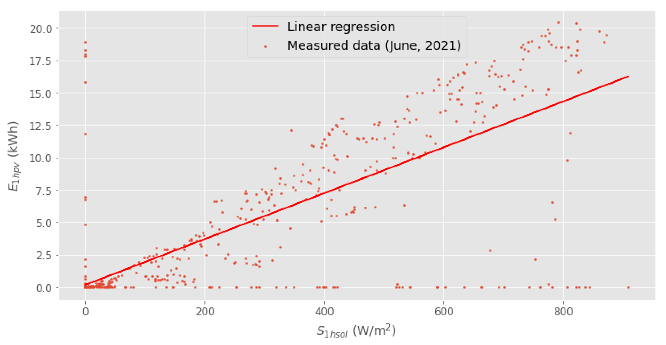
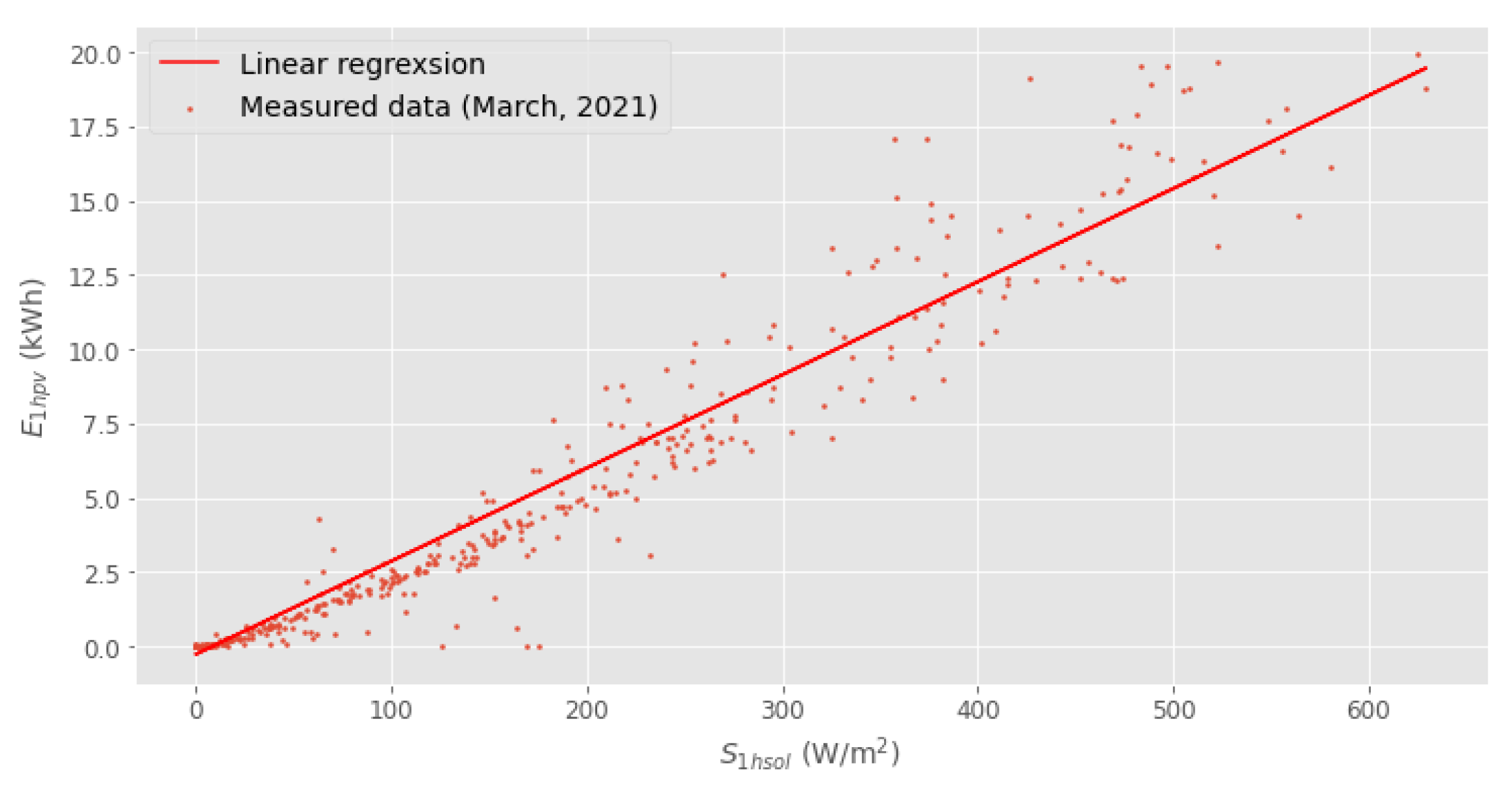
2.3.1. Correlations between Quantities Obtained from Different Sensors

In the further part of the article, examples of analysis of data obtained from measuring instruments installed in the described VPP are presented. First, we compare the data recorded by the pyranometer of the weather station, i.e., the intensity of solar radiation, and the total energy produced by the PV panels. The purpose of this comparison was not to build a predictive model, but to analyze the correlation between these quantities [31]. This study enabled to evaluate consistency of various data sources included in the virtual power plant. For the quantitative determination of the amount of radiant energy received by a PV module, it is necessary to convert the solar radiation density $S_{horiz}$ incident on the horizontal measuring plane of the pyranometer into the radiation density $S_{mod}$ incident on the PV module plane tilted to the horizontal plane by inclination angle $\beta$, assuming that the panels are facing south (azimuth = 180 degrees). For the daily analysis, the following relationships are valid [32]:

$$S_{horiz}=S_{i}sin\left(\alpha \right),S_{mod}=S_{i}sin(\alpha +\beta ),$$

(1)

where: $S_i$—maximum solar radiation measured in the plane perpendicular to the sun’s rays, $\alpha$—sun elevation angle determined as:

$$\alpha =90-\varphi +\delta ,$$

(2)

where: $\varphi$—latitude, $\delta$—declination angle calculated in turn using the formula:

$$\delta ={23.45}^{\circ }sin\left[\frac{360}{365}(284+d)\right],$$

(3)

where: d—number of the day of the year for which the calculations are performed.

A different approach was used in this study. Since the study purpose was only to check the consistency of data recorded from different sensors, the Equations (1)–(3) necessary to determine the radiation density with respect to the PV module plane were not applied. Instead, an analysis of the correlation between the raw pyranometer readings and the total energy produced by the available PV modules was conducted. The research was performed in accordance with the following methodology:

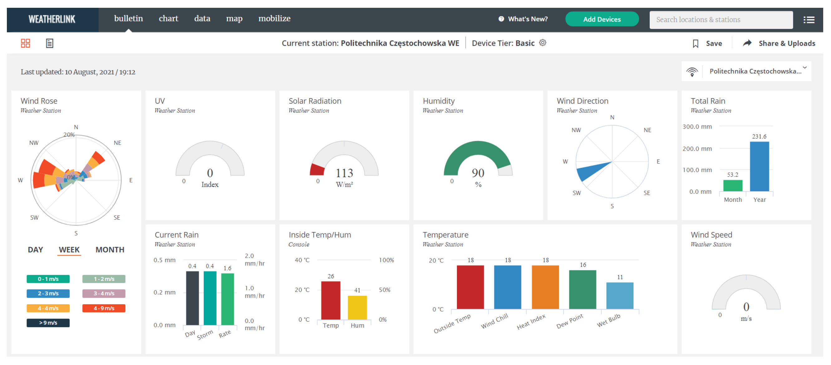
• Export of weather data from the WeatherLink application and data from the VRM portal to CSV files.
• Import of the data from CSV files to the Jupyter environment using the Pandas library [33,34].
• Data cleaning, including detection and completion of NaN values by interpolation.
• Averaging of the completed data series over one-hour intervals.
• Selection of the data time range(s) for the analysis purpose.
• Fitting linear models for hourly data in the selected periods using the ScikitLearn machine learning library, estimation of correlation coefficients [35].
• Assessment of the fit quality and formulation of conclusions.

At the first step the measurement weather data from the WeatherLink and the electric data from the Victron service (VRM) were exported to text files in the CSV format. Next, the data were imported into the unified Python-based Jupyter computation environment that includes the NumPy, Pandas, Scikit-Learn and other libraries. An important stage was cleaning the data series from NaN (Not A Number) values representing data missing due to failures of the instruments or communication interfaces or incorrect operation of services.

The data taken for analysis were time series of two recorded quantities, i.e., the solar radiation intensity $S_{sol}\left(t\right)$, in W/m${}^2$, recorded in one-minute intervals and the total energy produced by the PV installation $E_{pv}\left(t\right)$, in Wh, obtained for 15 min intervals. The linear interpolation was applied to complete the missing values [36]. A missing value in the interval $[t_0,t_1]$ was determined using the formula:

$$\widehat{Y}\left(t\right)=Y_0+\frac{(Y_1-Y_0)}{t_1-t_0}(t-t_0),$$

(4)

where: $t_1$—time instant of occurrence of the last valid numerical value before the data gap, $t_2$—time instant of occurrence of the first valid numerical value after the data gap, $\widehat{Y}\left(t\right)$—interpolated value of the quantity ($S_{sol}$ lub $E_{pv}$), $Y_1,Y_2$—values of the quantity recorded at $t_1$ and $t_2$, respectively.

In the next stage of the analysis, the complete time series $S_{sol}\left(t\right)$ and $E_{pv}\left(t\right)$ without NaN values were aggregated over a defined time interval. For the purpose of this study, the one-hour aggregating interval was specified. The new time series $S_{1hsol}$ representing the one-hour averaged values of the solar radiation were calculated as:

$$S_{1hsol}=\frac{1}{60}\sum _{t_{start}}^{t_{stop}}{S}_{sol}\left(t\right),$$

(5)

where: $t_{start},t_{stop}$—the beginning and the end time of the data averaging interval.

The data recorded in March and June of 2021 were selected for the analysis. The data was analyzed for the correlation between the average one-hour solar radiation intensity and the one-hour energy production from PV modules. A linear dependence of the energy production $E_{1hpv}$ on the radiation intensity was assumed:

$${\widehat{E}}_{1hpv}=w_0+w_1{S}_{1hsol},$$

(6)

where: $\mathbf{w}=(w_0,w_1)$—coefficient vector, ${\widehat{E}}_{1hpv},Wh$—estimator of the energy production.

To determine the coefficients in (6), the least squares method was used to obtain the best fit of the linear model by minimizing the sum of squared residuals between the measured values and the values predicted by the linear approximation (6) [31]:

$$\underset{\mathbf{w}}{min}=\parallel {S_{1hsol}\mathbf{w}-{\widehat{E}}_{1hpv}\parallel }_2^2,$$

(7)

where: $\parallel {\dots \parallel }_2^2$—square norm.

The calculations were performed in Python using the Scikit-learn machine learning library. In addition to the model coefficients, the linear correlation coefficient, the coefficient of determination and typical error measures such as MAE, MSE and RMSE [37] were determined. The results of the regression analysis are presented later in this article.

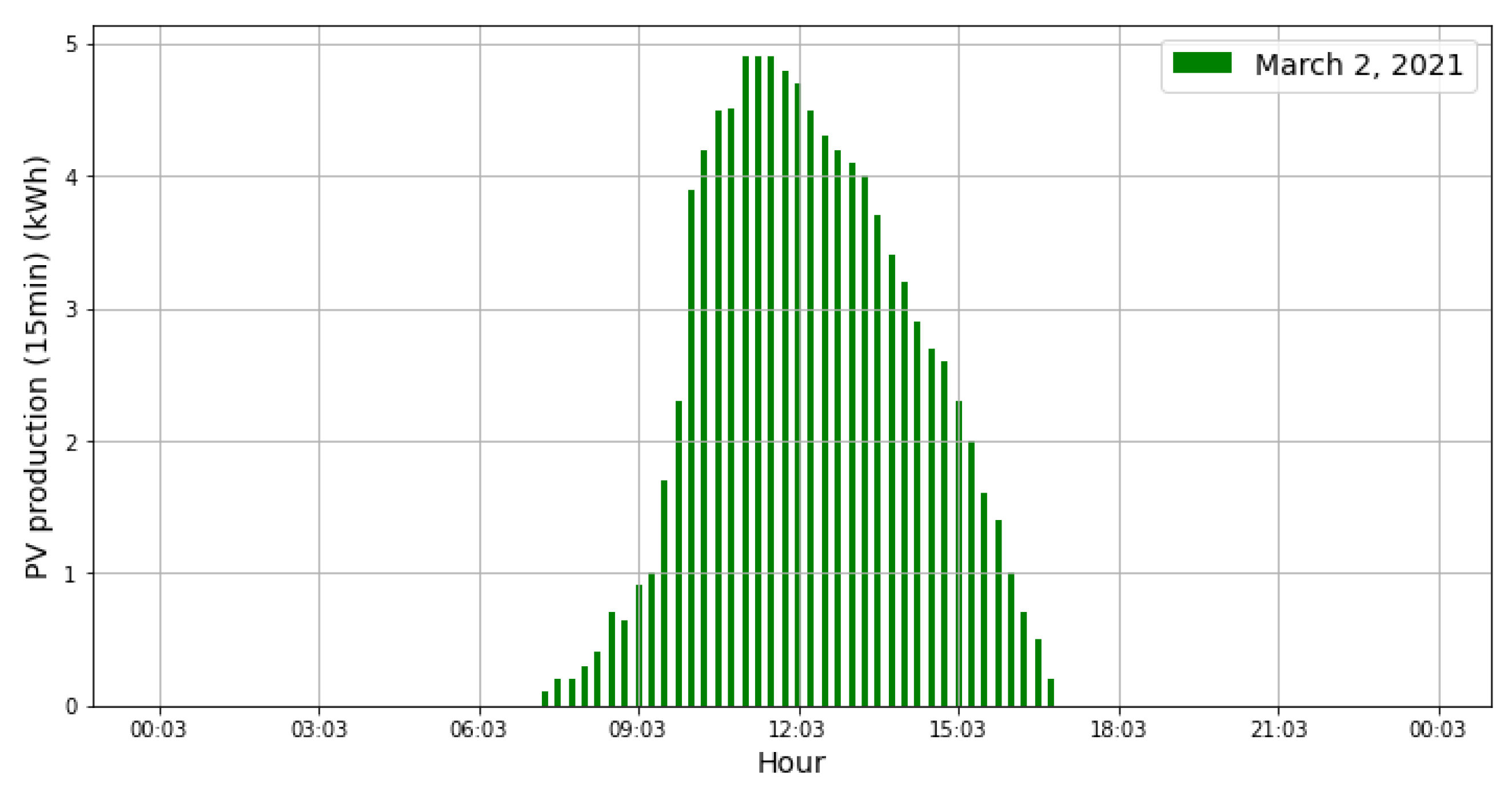
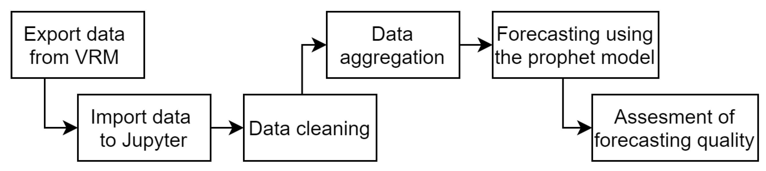
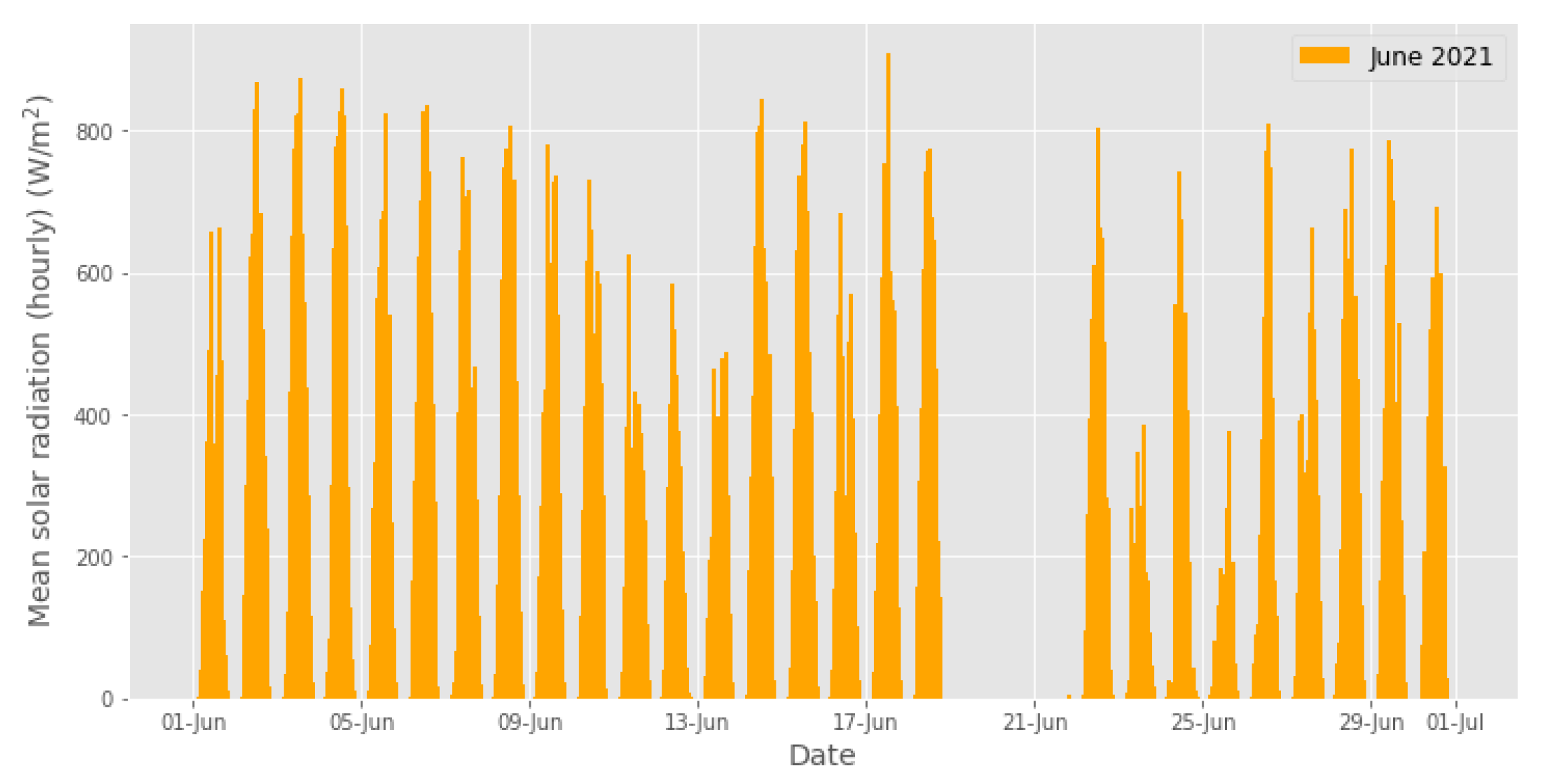
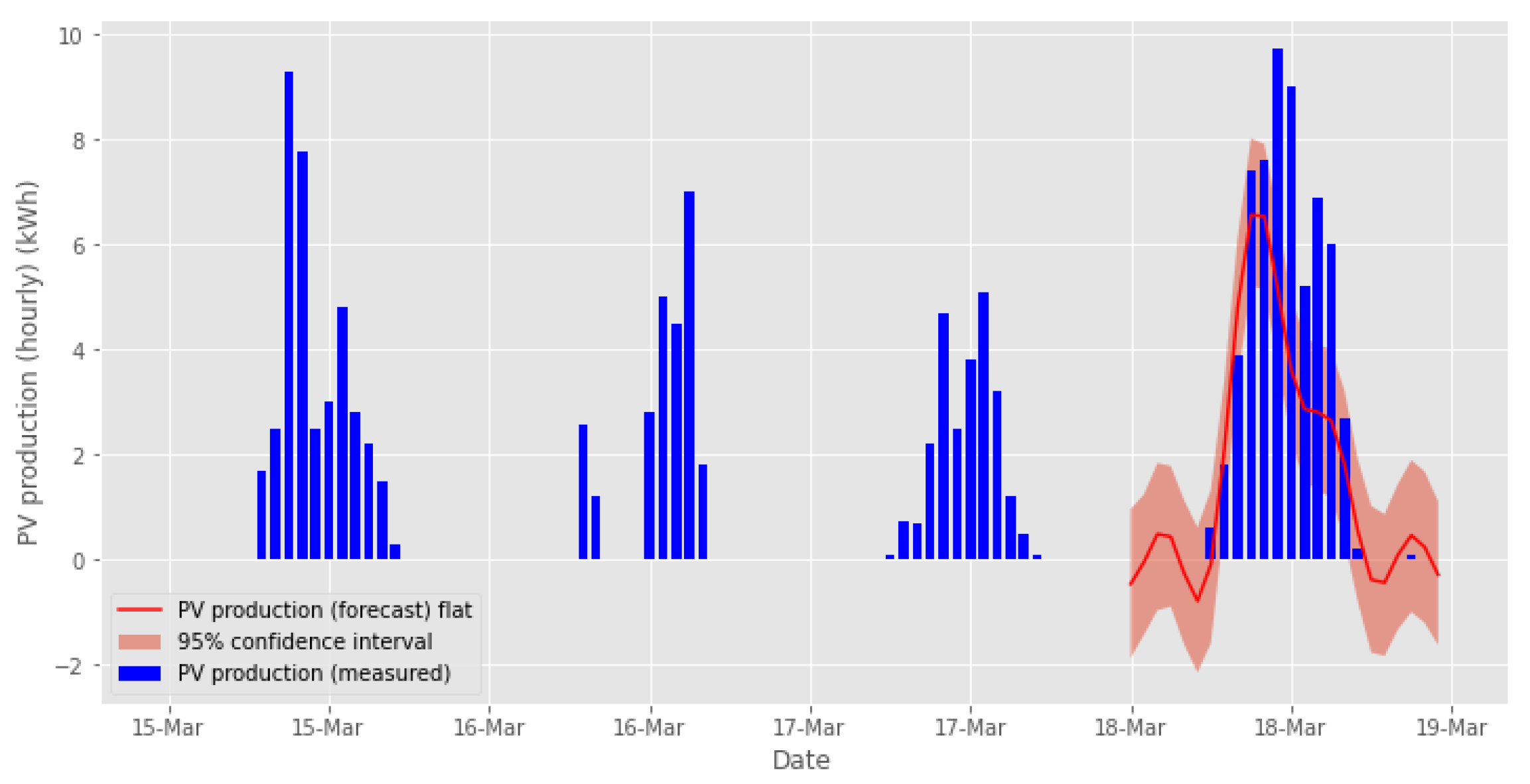
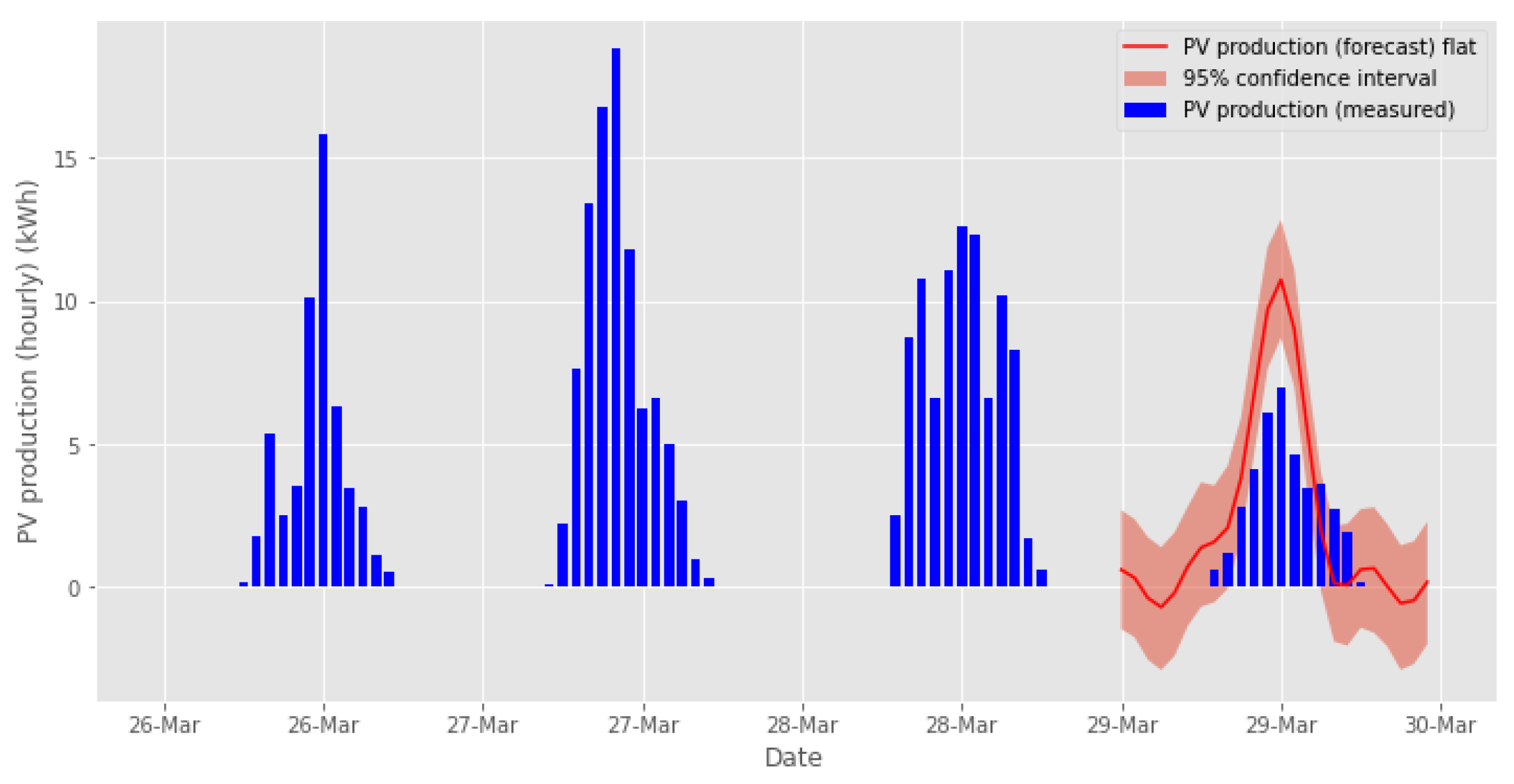
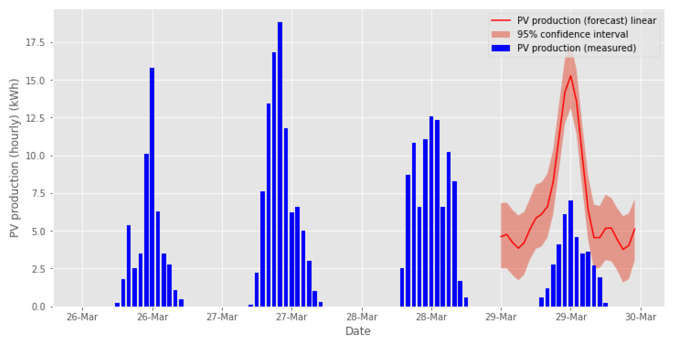
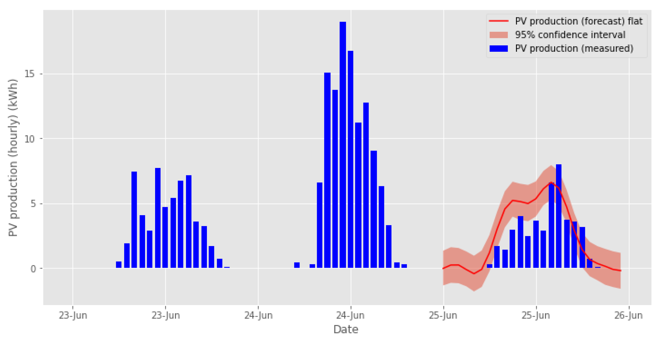
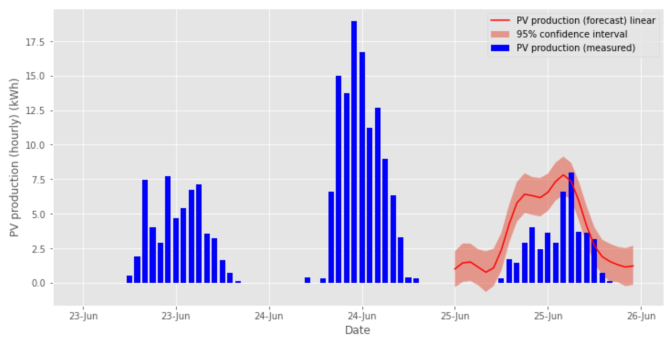
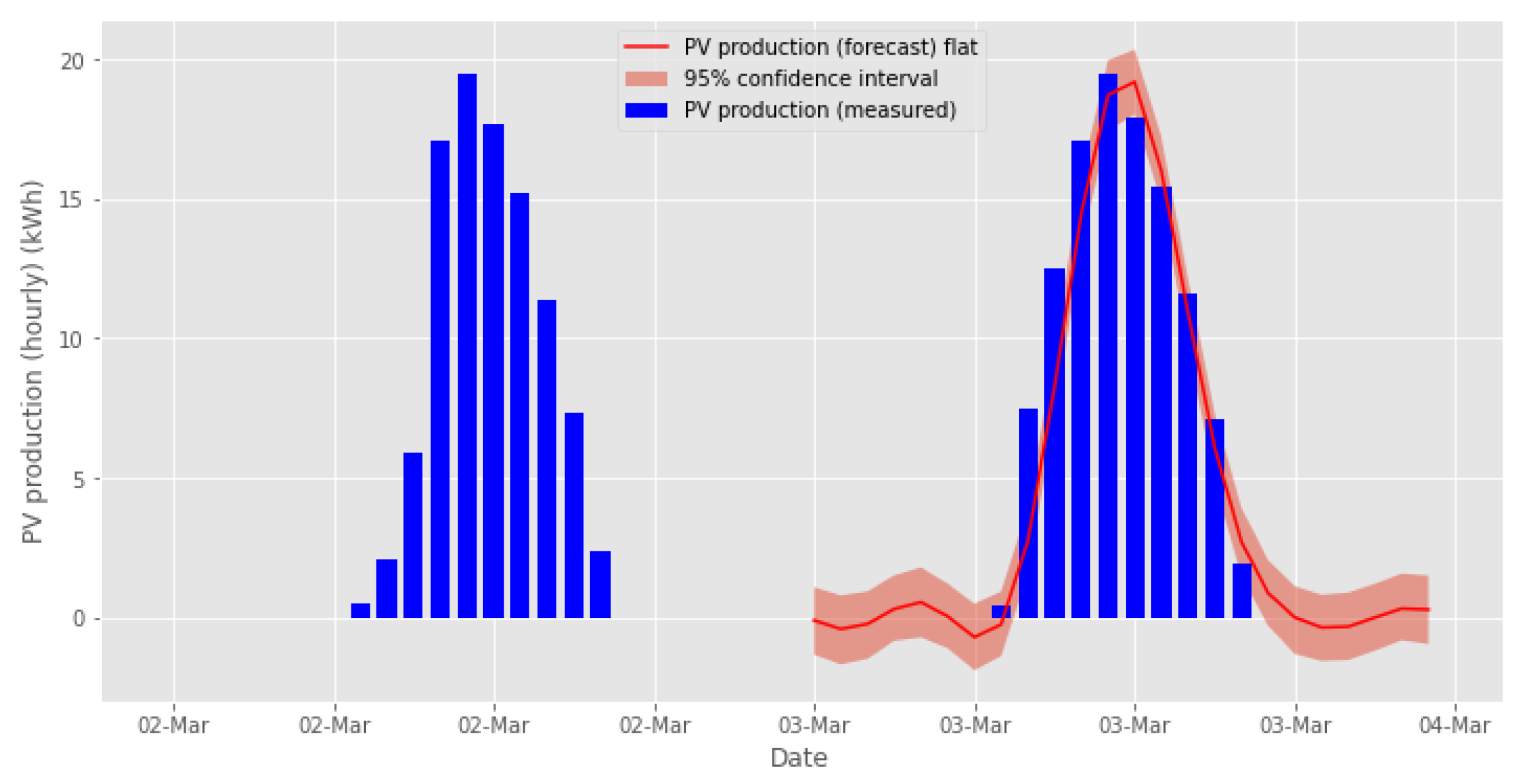
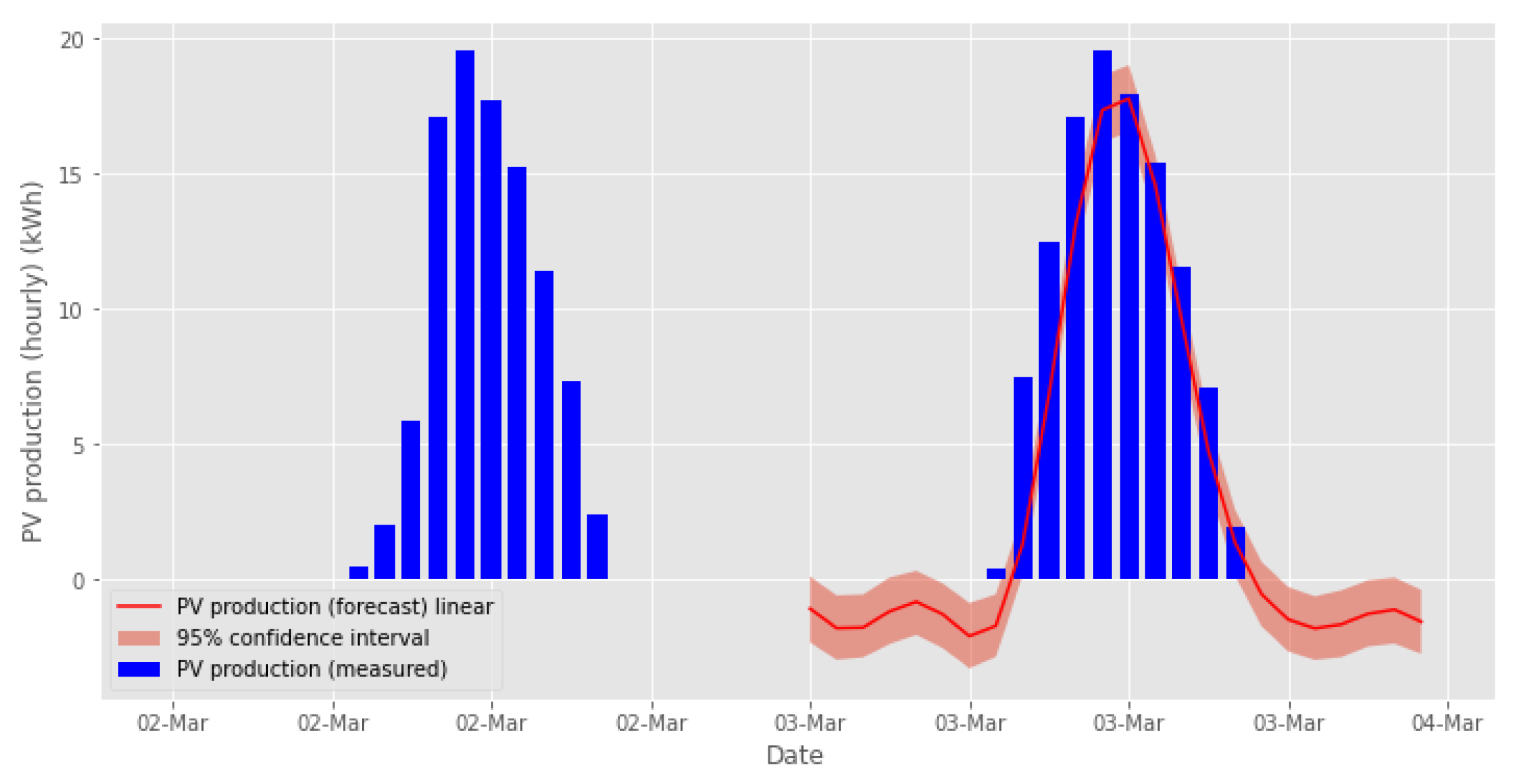
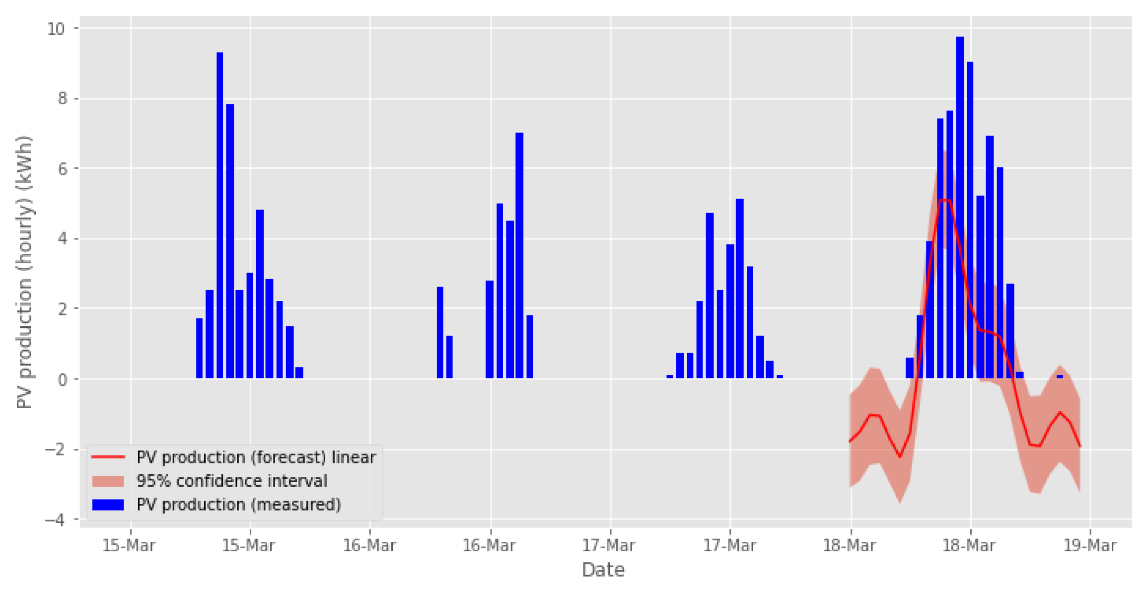
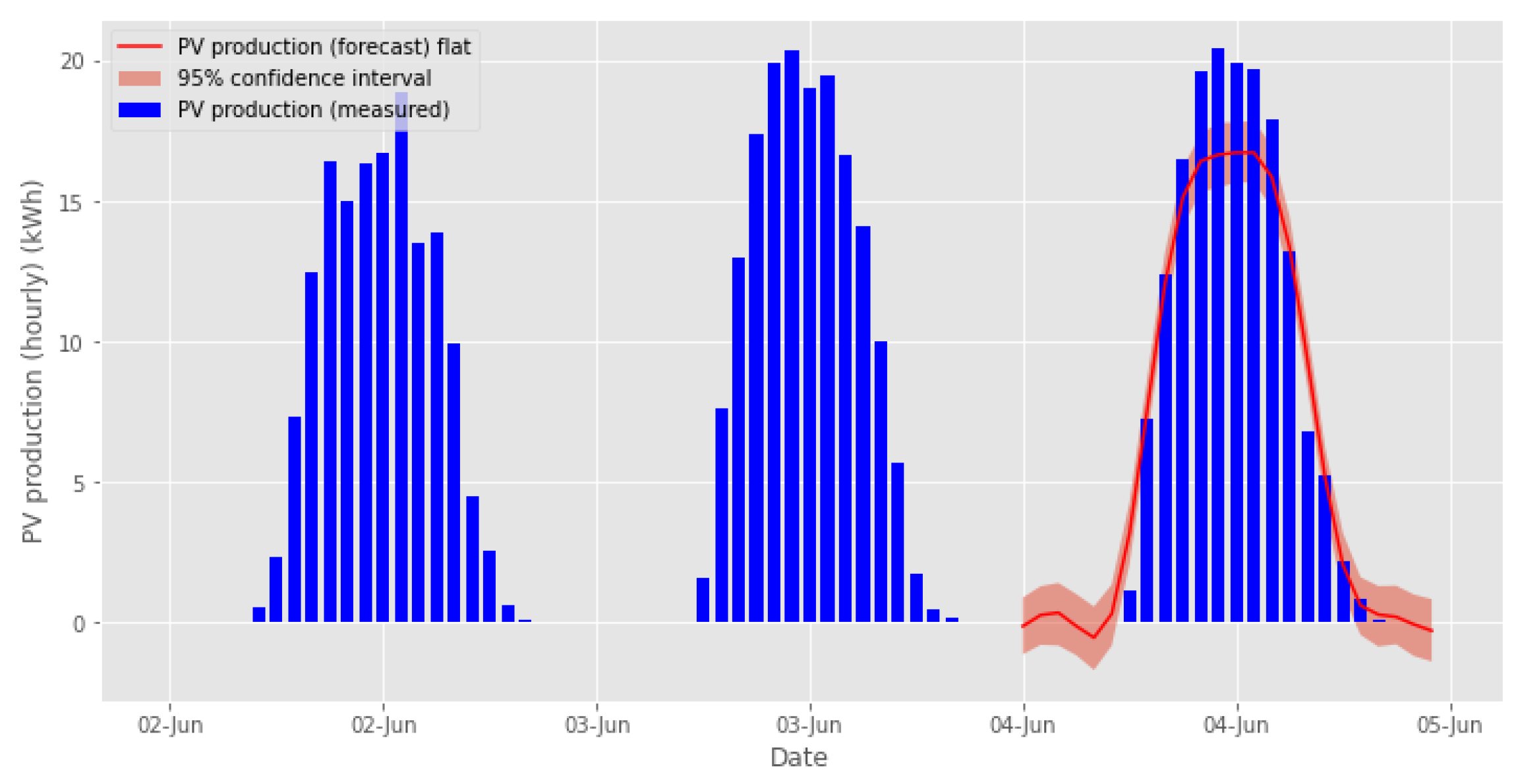
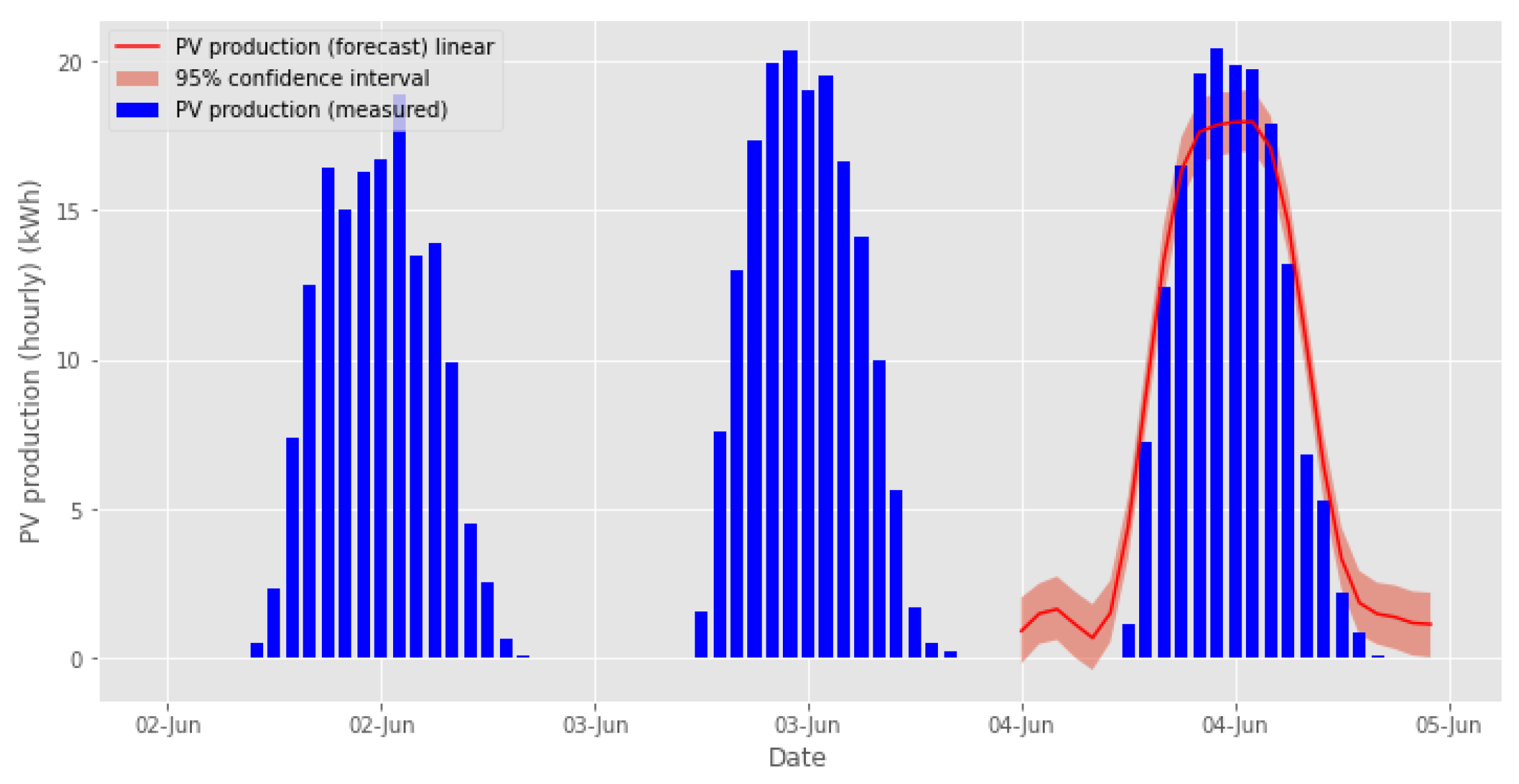
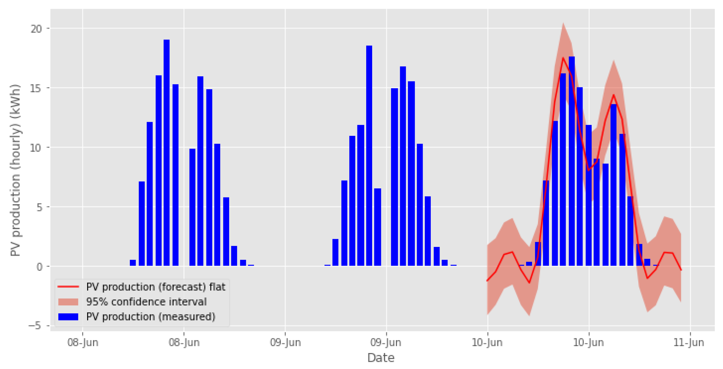
2.3.2. Prediction of Energy Production

Forecasting energy production from PV panels is presented as the second example of using data from the presented VPP. There are many time series forecasting methods used to forecast PV energy production, including: Autoregressive Moving Average (ARMA), Autoregressive Integrated Moving Average (ARIMA) or Seasonal Autoregressive Integrated Moving Average (SARIMA) [37,38]. In this work, the prophet forecasting model developed by Facebook employees [39] was used. The method allows a practical approach to “scale” at scale forecasting, which combines configurable models with performance analytics. Ref. [39] proposes a modular regression model with interpretable parameters that can be adjusted by analysts with domain knowledge about time. In this work, the analysis of time series in terms of forecasting PV energy production was carried out in the following stages:

• Export data from VRM installation to CSV files;
• Data import from CSV files to Jupyter environment using Pandas library;
• Data cleaning, including the detection and completion of NaN values with the use of interpolation;
• Data aggregation into hourly intervals;
• Selection of sample time periods for the purposes of the analysis;
• Application of the prophet forecasting model and “at scale” approach to energy production forecasting;
• Assessment of forecasting quality and formulation of conclusions.

The flowchart of the research methodology is depicted in Figure 15.

The first six steps of data analysis are described in Section 2.3.1, while the prophet forecasting model is presented below.

The Prophet prediction model is based on the time series model proposed by Harvey and Peters in [40]:

$$y\left(t\right)=g\left(t\right)+s\left(t\right)+h\left(t\right)+{ϵ}_t$$

(8)

where: $g\left(t\right)$ is a trend function that models non-periodic changes in the value of the series, $s\left(t\right)$ models periodic changes (e.g., weekly and annual seasonality), $h\left(t\right)$ models effects of holidays, ${ϵ}_t$ represents an error, which is assumed to be normally distributed nym. In model (8), you can easily adjust the multi-period seasonality and also allow the analyst to test various assumptions about trends. In addition, unlike ARIMA models, the measurements do not need to be regularly spaced, and there is no need to interpolate missing values. An important feature of the method is the quick fit of the model. Ultimately, the model has easily interpreted parameters and can easily be extended with new components.

In the Prophet model, two trend functions representing non-periodic changes in the value of the time series were proposed, i.e.,: a non-linear growth model with saturation and a linear trend with change points that can be selected automatically or by an analyst. The nonlinear growth model with saturation expresses the following dependence:

$$g\left(t\right)=\frac{C}{1+{\mathrm{e}}^{-k(t-m)}},$$

(9)

where: C—the carrying capacity, k—the growth rate, m—an offset parameter. A detailed description of the linear trend model can be found in [39].

The seasonal component, depending on (8), was modeled on the basis of the Fourier series in the form:

$$s\left(t\right)=\sum _{n=1}^N\left(a_{n}cos\left(\frac{2\pi nt}{P}\right)+b_{n}sin\left(\frac{2\pi nt}{P}\right)\right),$$

(10)

where: P—expected period (e.g., $P=7$ in the case of weekly seasonality).

To determine the seasonality with the use of approximation (10), it is necessary to estimate the vector of $2n$ parameters:

$$\beta =[a_1,b_1,\dots a_n,b_n].$$

(11)

The model fit operation is performed on the basis of a matrix of seasonality vectors computed for each $t\text{-}value$ for historical and future data. For example, if we want to model the annual seasonality for $N=3$, the form of the matrix of seasonality vectors is expressed by the following formula [39]:

$$\mathbf{X}\left(t\right)=[cos\left(\frac{2\pi \left(1\right)t}{365.25}\right)+sin\left(\frac{2\pi \left(3\right)t}{365.25}\right)]$$

(12)

Apart from the trend (9) and seasonality (10) models, the Prophet model introduces the option of taking into account the Christmas event. However, in this study, only the above-described components of the model were used to forecast energy production by PV modules (8). The results of the forecasts are presented later in this paper.

3. Results

In the further part of the article exemplary results of the analysis of data obtained from the described VPP are presented and discussed. The recorded profiles of the aggregated hourly PV energy production in March and June of 2021 are shown in Figure 16 and Figure 17, respectively. Figure 18 and Figure 19 show the average hourly solar radiation intensity recorded over the same two months. One can see large daily fluctuations of these two correlated quantities in March, 2021. Two gaps in the energy production on 20 June and 27 (Figure 17) resulted from the system failures. The PV installation did not produce electricity on these two days. Another result of the system failure is that the weather data for 19–21 June was also not recorded (Figure 19).

The analysis of correlation between the average hourly solar radiation intensity recorded by the pyranometer and the hourly PV energy production in March and June of 2021 are shown as the linear regression fits in Figure 20 and Figure 21 respectively. A large number of outliers on the graph in Figure 21 is noteworthy. The points, for which the energy production $E_{1hpv}$ is zero, occur due to the aforementioned system failure and a break in the electricity production, while the solar radiation data were still measured. Similarly, the points for which $S_{1hsol}$ is zero, but at the same time the electricity production is non-zero, occur due to the lack of meteorological data.

Exemplary results of the PV plant energy production forecasting using the Prophet Forecasting Model (8) described above and the data recorded at the CUT VPP are presented in Figure 22, Figure 23, Figure 24, Figure 25, Figure 26, Figure 27, Figure 28, Figure 29, Figure 30, Figure 31, Figure 32 and Figure 33. The study was carried out using the methodology described in Section 2.3.2. The presented results concern three selected days of March and three days of June, 2021, assuming a flat and a linear trend (12 cases in total). The graphs present the one-day-ahead hourly forecasts (red plot) with corresponding 95% confidence intervals (orange strip) against the actual data (blue bar graph for the same day) and the earlier data used as learning datasets (blue bar graphs). For March 3, the learning set included data from a day before (Figure 22 and Figure 23), for March 18 (Figure 24 and Figure 25) and March 29 (Figure 26 and Figure 27) the learning set included data from three days before.

For 4 June (Figure 28 and Figure 29), 10 June (Figure 30 and Figure 31) and 25 June (Figure 32 and Figure 33) the learning set included data from two days before.

As can be seen in Figure 22 and Figure 33, the forecasts cover the next 24 h, including the hours when the energy production is known to be zero—at night the solar radiation is zero and the PV plant does not work. The authors are aware of the weakness of the algorithm in this regard. However, one of the aims of this article was only to verify the validity of using the Prophet Forecasting Model to forecast electricity production by a PV power plant. Analyzing graphs in Figure 22 and Figure 33, it can be noticed that more accurate forecasts were obtained for a flat trend model.

4. Discussion and Conclusions

The results of the regression analysis for March and June, 2021, presented in Figure 20 and Figure 21 and in

Table 1. Parameters for assessing accuracy of the linear approximation of the PV plant energy production vs. the insolation level.

	MAE	MSE	RMSE	R${}^2$
	(kWh)	(kWh)	(kWh)	-
March 2021	0.62	1.07	1.03	0.95
June 2021	1.97	12.79	3.58	0.64

, show that the insolation level was more stable in March. This is also confirmed by the coefficient of determination: for the March data R${}^2$ = 0.95, for the June data R${}^2$ = 0.64.

It should be pointed out that determining the parameters from Table 1 is important when selecting the length of the sequences that are used to train a prognostic model. If the coefficient of determination from is too low (below 0.8), the training sequences should be shortened to improve the prediction accuracy. To support this conclusion, we conducted cross-validation of the MAE prediction errors for various periods—from 1 to 15 days—of the model training. The results of this analysis are presented in Figure 34 for March and in Figure 35 for June 2021. The decrease of the MAE with shortening of the learning period is clearly visible in Figure 35 because the coefficient of determination for the June data is low. However, this is not a rule for the plots in Figure 34 because the coefficient of determination for the March data is high, which confirms the above thesis.

The VPP data analysis carried out in Section 3 clearly indicates that an important factor affecting the prediction accuracy of the used model (8) is appropriate selection of assumed trend function $g\left(t\right)$. In all the presented cases, the MSE and MAE errors for a flat trend function, presented in

Table 2. Forecasting accuracy errors assuming a flat trend function.

	MSE	MAE
	(kWh)	(kWh)
3 March	2.29	0.91
18 March	3.72	1.21
29 March	3.24	1.33
4 June	2.56	1.04
10 June	2.75	1.32
25 June	1.93	0.97

, are lower than the corresponding errors for a linear trend function, presented in

Table 3. Forecasting accuracy errors assuming a linear trend function.

	MSE	MAE
	(kWh)	(kWh)
3 March	5.60	1.88
18 March	8.75	2.43
29 March	28.9	5.1
4 June	2.84	1.49
15 June	41.7	6.25
25 June	4.70	1.83

.

We suppose that in further experiments, we should go towards models with a spline trend function $g\left(t\right)$, which would allow for combining the advantages of both linear and nonlinear functions.

The forecasting accuracy is significantly affected by the quality of historical data and occurrence of the system failures. In Table 1, we can see significantly greater forecasting errors for the June data because, as it was mentioned earlier, on two days of June 2021 the PV power plant was out of operation due to the system failure. For March, when the electricity production remained uninterrupted, the forecasting errors are much lower. The biggest difference occurs in the case of the MSE error.

It should be noted that in this work, we were verifying the statistical model that had been used so far for social and business research. The authors decided to apply it to technical analysis purposes, more specifically for prediction of electricity production at a photovoltaic farm. The next step in the development of the algorithm, which is now based only on the historical energy production time series, will be its extension by adding elements related to the physics of the phenomenon, like the insolation level time series. Currently, the model provides forecasts also for the night hours, when the PV power plant is out of operation. These values are different from zero, which deteriorates the forecast accuracy. In the authors’ opinion, limiting the forecast only to the day hours, when the PV plant is in operation, will have a positive impact on the forecast accuracy. An appropriate further research and tests will show to what extent.

References

1. European Commission. A Clean Planet for all A European Strategic Long-Term Vision for a Prosperous, Modern, Competitive and Climate Neutral Economy; Directorate-General for Climate Action: Brussels, Belgium, 2018. [Google Scholar]
2. Statistics Poland. Energy from Renewable Sources in 2019; Department of Statistical Publishing: Warsaw, Poland, 2020. [Google Scholar]
3. Asmus Microgrids, P. Virtual power plants and our distributed energy future. Elektr. J. 2010, 23, 72–82. [Google Scholar]
4. Su, W.; Wang, J. Energy management systems in microgrid operations. Elektr. J. 2016, 25, 45–60. [Google Scholar] [CrossRef]
5. Kardakos, E.G.; Simoglou, C.K.; Bakirtzis, A.G. Optimal offering strategy of a virtual power plant: A stochastic bi-level approach. IEEE Trans. Smart Grid 2016, 7, 794–806. [Google Scholar] [CrossRef]
6. Rahimiyan, M.; Baringo, L. Strategic bidding for a virtual power plant in the day-ahead and real-time markets: A price-taker robust optimization approach. IEEE Trans. Power Syst. 2016, 31, 2676–2687. [Google Scholar] [CrossRef]
7. Mashhour, E.; Moghaddas-Tafreshi, S.M. Bidding strategy of virtual power plant for participating in energy and spinning reserve markets—Part I: Problem formulation. IEEE Trans. Power Syst. 2011, 26, 949–956. [Google Scholar] [CrossRef]
8. Sarker, M.R.; Dvorkin, Y.; Ortega-Vazquez, M.A. Optimal participation of an electric vehicle aggregator in day-ahead energy and reserve markets. IEEE Trans. Power Syst. 2016, 31, 3506–3515. [Google Scholar] [CrossRef]
9. Giuntoli, M.; Poli, D. Optimized thermal and electrical scheduling of a large scale virtual power plant in the presence of energy storages. IEEE Trans. Smart Grid 2013, 4, 942–955. [Google Scholar] [CrossRef]
10. Jasiński, M.; Sikorski, T.; Kaczorowska, D.; Rezmer, J.; Suresh, V.; Leonowicz, Z.; Kostyla, P.; Szymańda, J.; Janik, P. A Case Study on Power Quality in a Virtual Power Plant: Long Term Assessment and Global Index Application. Energies 2020, 13, 6578. [Google Scholar] [CrossRef]
11. Moutis, P.; Georgilakis, P.S.; Hatziargyriou, N.D. Voltage regulation support along a distribution line by a virtual power plant based on a center of mass load modeling. IEEE Trans. Smart Grid. 2018, 9, 3029–3038. [Google Scholar] [CrossRef]
12. Moutis, P.; Hatziargyriou, N.D. Decision trees-aided active power reduction of a virtual power plant for power system over-frequency mitigation. IEEE Trans. Ind. Informat. 2015, 11, 251–261. [Google Scholar] [CrossRef]
13. Popławski, T.; Szelag, P.; Bartnik, R. Adaptation of models from determined chaos theory to short-term power forecasts for wind farms. Bull. Pol. Acad. Sci. Tech. Sci. 2020, 68, 1491–1501. [Google Scholar] [CrossRef]
14. Wang, J.; Wang, Y.; Li, Y. A novel hybrid strategy using three-phase feature extraction and a weighted regularized extreme learning machine for multi-step ahead wind speed prediction. Energies 2018, 11, 321. [Google Scholar] [CrossRef] [Green Version]
15. Pal, P.; Krishnamoorthy, P.A.; Rukmani, D.K.; Antony, S.J.; Ocheme, S.; Subramanian, U.; Elavarasan, R.M.; Das, N.; Hasanien, H.M. Optimal Dispatch Strategy of Virtual Power Plant for Day-Ahead Market Framework. Appl. Sci. 2021, 11, 3814. [Google Scholar] [CrossRef]
16. Behi, B.; Baniasadi, A.; Arefi, A.; Gorjy, A.; Jennings, P.; Pivrikas, A. Cost–Benefit Analysis of a Virtual Power Plant Including Solar PV, Flow Battery, Heat Pump, and Demand Management: A Western Australian Case Study. Energies 2020, 13, 2614. [Google Scholar] [CrossRef]
17. Pasetti, M.; Rinaldi, S.; Manerba, D. A Virtual Power Plant Architecture for the Demand-Side Management of Smart Prosumers. Appl. Sci. 2018, 8, 432. [Google Scholar] [CrossRef] [Green Version]
18. Zidane, T.E.K.; Adzman, M.R.; Tajuddin, M.F.N.; Zali, S.M.; Durusu, A.; Mekhilef, S. Optimal Design of Photovoltaic Power Plant Using Hybrid Optimisation: A Case of South Algeria. Energies 2020, 13, 2776. [Google Scholar] [CrossRef]
19. Choi, Y. Solar Power System Planning and Design. Appl. Sci. 2021, 10, 367. [Google Scholar] [CrossRef] [Green Version]
20. Moreno-Garcia, I.M.; Palacios-Garcia, E.J.; Pallares-Lopez, V.; Santiago, I.; Gonzalez-Redondo, M.J.; Varo-Martinez, M.; Real-Calvo, R.J. Real-Time Monitoring System for a Utility-Scale Photovoltaic Power Plant. Sensors 2016, 16, 770. [Google Scholar] [CrossRef] [PubMed] [Green Version]
21. Beránek, V.; Olšan, T.; Libra, M.; Poulek, V.; Sedláček, J.; Dang, M.-Q.; Tyukhov, I.I. New Monitoring System for Photovoltaic Power Plants’ Management. Energies 2018, 11, 2495. [Google Scholar] [CrossRef] [Green Version]
22. Ansari, S.; Ayob, A.; Lipu, M.S.H.; Saad, M.H.M.; Hussain, A. A Review of Monitoring Technologies for Solar PV Systems Using Data Processing Modules and Transmission Protocols: Progress, Challenges and Prospects. Sustainability 2021, 13, 8120. [Google Scholar] [CrossRef]
23. Järvelä, M.; Valkealahti, S. Ideal Operation of a Photovoltaic Power Plant Equipped with an Energy Storage System on Electricity Market. Appl. Sci. 2017, 7, 749. [Google Scholar] [CrossRef] [Green Version]
24. Satya Prakash Oruganti, K.; Aravind Vaithilingam, C.; Rajendran, G. Design and Sizing of Mobile Solar Photovoltaic Power Plant to Support Rapid Charging for Electric Vehicles. Energies 2019, 12, 3579. [Google Scholar] [CrossRef] [Green Version]
25. Wrobel, K.; Tomczewski, K.; Sliwinski, A.; Tomczewski, A. Optimization of a Small Wind Power Plant for Annual Wind Speed Distribution. Energies 2021, 14, 1587. [Google Scholar] [CrossRef]
26. Lehneis, R.; Manske, D.; Thrän, D. Modeling of the German Wind Power Production with High Spatiotemporal Resolution. Int. J. Geo-Inf. 2021, 10, 104. [Google Scholar] [CrossRef]
27. Meegahapola, L.; Bu, S. Special Issue: “Wind Power Integration into Power Systems: Stability and Control Aspects”. Energies 2021, 14, 3680. [Google Scholar] [CrossRef]
28. Yan, X.; Yang, L.; Li, T. The LVRT Control Scheme for PMSG-Based Wind Turbine Generator Based on the Coordinated Control of Rotor Overspeed and Supercapacitor Energy Storage. Energies 2021, 14, 518. [Google Scholar] [CrossRef]
29. Gała, M.; Jąderko, A. Assessment of the impact of photovoltaic system on the power quality in the distribution network. PrzegląD Elektrotechniczny 2018, 12, 162–165. [Google Scholar] [CrossRef]
30. Solutions & Co. Available online: http://www.solutionsandco.org/project/aquion-energy/ (accessed on 28 July 2021).
31. Bevington Philip, R.; Robinson Keith, D. Data Reduction and Error Analysis for the Physical Sciences; McGraw-Hill: New York, NY, USA, 2003. [Google Scholar]
32. Luque, A.; Hegedus, S.; Preiser, K. (Eds.) Photovoltaic Systems. In Handbook of Photovoltaic Science and Engineering; John Willey & Sons Ltd.: Hoboken, NJ, USA, 2003. [Google Scholar]
33. Jupyter Project. Available online: https://jupyter.org/ (accessed on 22 August 2021).
34. McKinney, W. Data structures for statistical computing in python. In Proceedings of the 9th Python in Science Conference, Austin, TX, USA, 28 June–3 July 2010; Volume 445, pp. 56–61. [Google Scholar]
35. Pedregosa, F.; Varoquaux, G.; Gramfort, A.; Michel, V.; Thirion, B.; Grisel, O.; Blondel, M.; Prettenhofer, P.; Weiss, R.; Dubourg, V.; et al. Scikit-learn: Machine Learning in Python. J. Mach. Learn. Res. 2011, 12, 2825–2830. [Google Scholar]
36. Bayen, A.M.; Siauw, T. An Introduction to MATLAB® Programming and Numerical Methods for Engineers; Elsevier Inc.: Amsterdam, The Netherlands, 2015. [Google Scholar]
37. Nespoli, A.; Ogliari, E.; Leva, S.; Massi Pavan, A.; Mellit, A.; Lughi, V.; Dolara, A. Day-Ahead Photovoltaic Forecasting: A Comparison of the Most Effective Techniques. Energies 2019, 12, 1621. [Google Scholar] [CrossRef] [Green Version]
38. Percival, D.B.; Walden, A.T. Spectral Analysis for Physical Applications; Cambridge University: Cambridge, UK, 1993. [Google Scholar]
39. Taylor, S.J.; Letham, B. Forecasting at scale. PeerJ Prepr. 2017, 5, e3190v2. [Google Scholar] [CrossRef]
40. Harvey, A.; Peters, S. Estimation procedures for structural time series models. J. Forecast. 1990, 9, 89–108. [Google Scholar] [CrossRef]
Figure 1. Components making up the VPP at the FEE, CUT.
Energies 14 06200 g001
Figure 2. The wind farm and the photovoltaic power plant located on the roofs of the FEE, CUT buildings.
Energies 14 06200 g002
Figure 3. The FEE 45 kWp photovoltaic power plant.
Energies 14 06200 g003
Figure 4. The FEE 30 kWp wind power plant.
Energies 14 06200 g004
Figure 5. The 25 kWh energy storage installed in the FEE micro VPP. Source: [30].
Energies 14 06200 g005
Figure 6. System monitoring in the Victron Remote Mangement software.
Energies 14 06200 g006
Figure 7. Historical data presented in the Victron Remote Mangement software.
Energies 14 06200 g007
Figure 8. Graphs showing what the energy from the photovoltaic installation was used for.
Energies 14 06200 g008
Figure 9. Graphs showing the breakdown of electricity transferred through the inverter’s guaranteed output by the source of origin.
Energies 14 06200 g009
Figure 10. Example set of widgets presenting historical data in the VRM application.
Energies 14 06200 g010
Figure 11. Fifteen-minute profile of PV energy production recorded on 2 March 2021.
Energies 14 06200 g011
Figure 12. Fifteen-minute profile of PV energy production recorded on 2 June 2021.
Energies 14 06200 g012
Figure 13. Monitoring of the current weather parameters via the www.weatherlink.com (accessed on 10 August 2021) portal.
Energies 14 06200 g013
Figure 14. The website panel for remote view and download of data stored in the Energia 4 application database.
Energies 14 06200 g014
Figure 15. The flowchart of the research methodology.
Energies 14 06200 g015
Figure 16. Hourly PV power plant energy production measured at the CUT VPP in March, 2021.
Energies 14 06200 g016
Figure 17. Hourly PV power plant energy production measured at the CUT VPP in June, 2021.
Energies 14 06200 g017
Figure 18. Average hourly solar radiation measured at the CUT VPP in March, 2021.
Energies 14 06200 g018
Figure 19. Average hourly solar radiation measured at the CUT VPP in March, 2021.
Energies 14 06200 g019
Figure 20. Linear regression model of correlation between the average hourly solar radiation and the hourly PV plant energy production for March, 2021.
Energies 14 06200 g020
Figure 21. Linear regression model of correlation between the average hourly solar radiation and the hourly PV plant energy production for June, 2021.
Energies 14 06200 g021
Figure 22. The PV plant energy production forecast for 3 March, on-day learning set, flat trend model.
Energies 14 06200 g022
Figure 23. The PV plant energy production forecast for 3 March, on-day learning set, linear trend model.
Energies 14 06200 g023
Figure 24. The PV plant energy production forecast for 18 March, three-day learning set, flat trend model.
Energies 14 06200 g024
Figure 25. The PV plant energy production forecast for 18 March, three-day learning set, linear trend model.
Energies 14 06200 g025
Figure 26. The PV plant energy production forecast for 29 March, three-day learning set, flat trend model.
Energies 14 06200 g026
Figure 27. The PV plant energy production forecast for 29 March, three-day learning set, linear trend model.
Energies 14 06200 g027
Figure 28. The PV plant energy production forecast for 4 June, two-day learning set, flat trend model.
Energies 14 06200 g028
Figure 29. The PV plant energy production forecast for 4 June, two-day learning set, linear trend model.
Energies 14 06200 g029
Figure 30. The PV plant energy production forecast for 10 June, two-day learning set, flat trend model.
Energies 14 06200 g030
Figure 31. The PV plant energy production forecast for 10 June, two-day learning set, linear trend model.
Energies 14 06200 g031
Figure 32. The PV plant energy production forecast for 25 June, two-day learning set, flat trend model.
Energies 14 06200 g032
Figure 33. The PV plant energy production forecast for 25 June, two-day learning set, linear trend model.
Energies 14 06200 g033
Figure 34. Plots of the MAE prediction error vs. the prediction horizon obtained from cross-validation for the March 2021 data.
Energies 14 06200 g034
Figure 35. Plots of the MAE prediction error vs. the prediction horizon obtained from cross-validation for the June 2021 data.
Energies 14 06200 g035