
Optimization Method for Multiple Measures to Mitigate Line Overloads in Power Systems

Abstract
:1. Introduction
2. Analysis of Protection and Control Measures
2.1. Controlling Values of Different Measures
2.2. Response Times of Different Measures
3. Mathematical Algorithms
3.1. PFT
3.2. BSO and IBSO
3.2.1. Introduction of BSO
3.2.2. Introduction of IBSO
4. Optimization Method for Multiple Measures
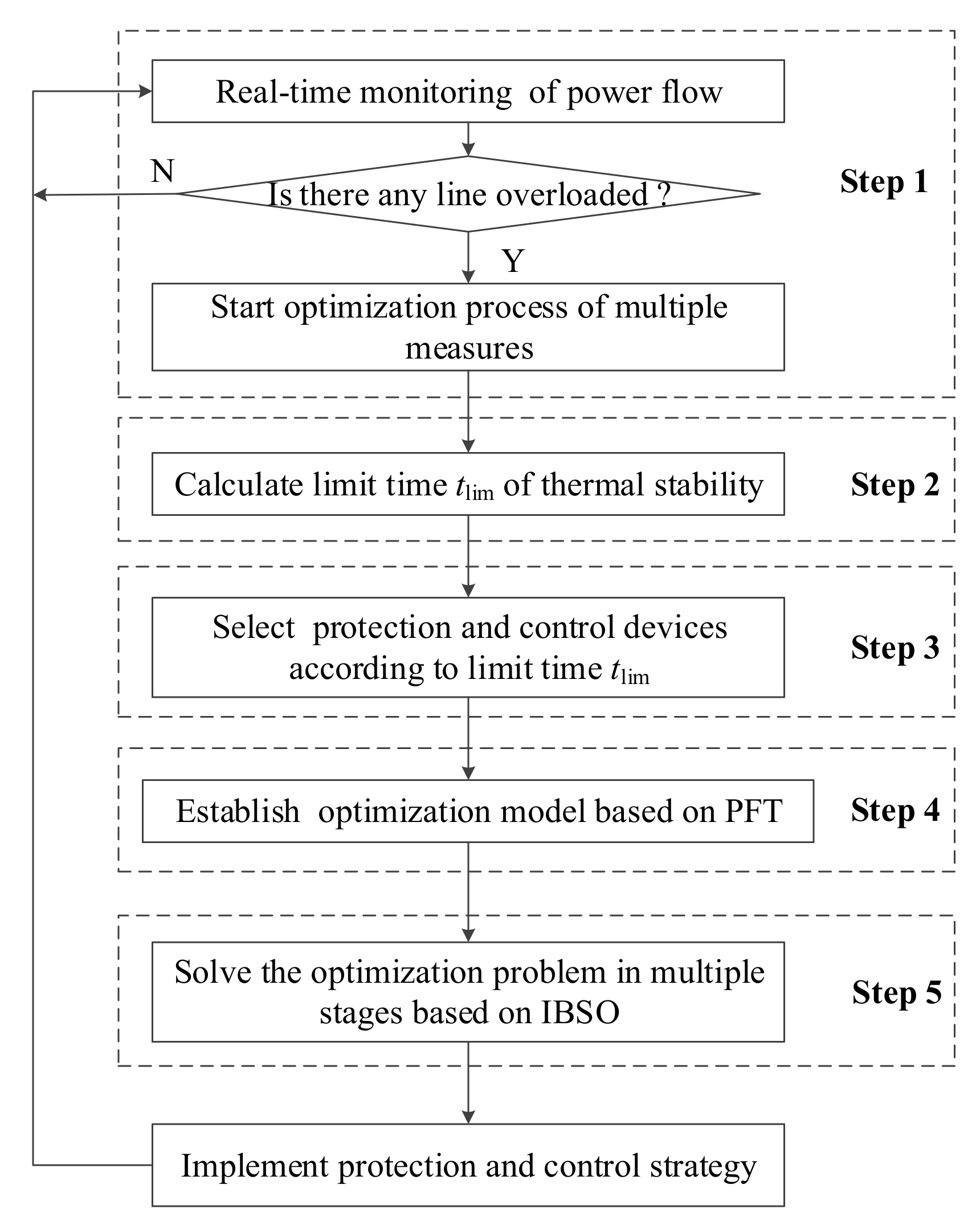
4.1. Process Overview
4.2. Modeling Process Based on PFT
4.3. Solving Process Based on IBSO
5. Test Cases
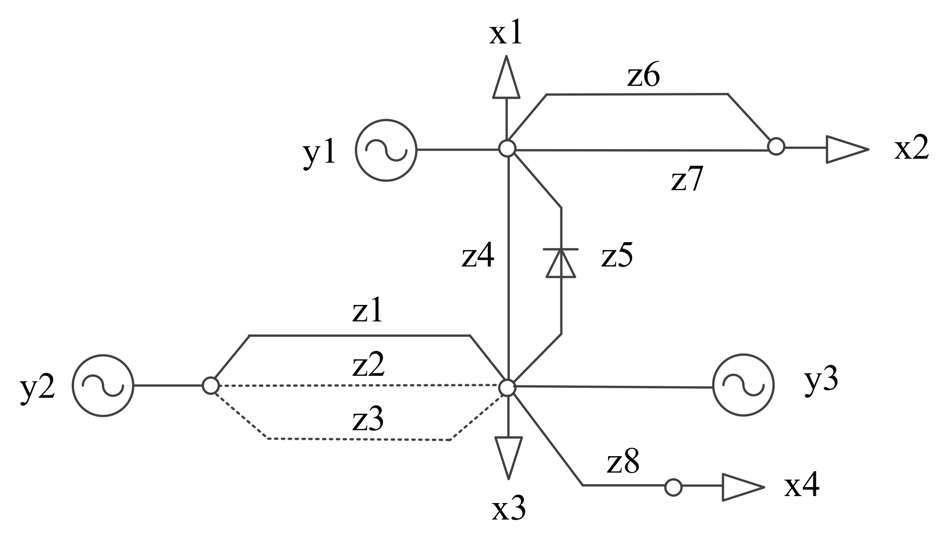
5.1. Five-Bus Test System
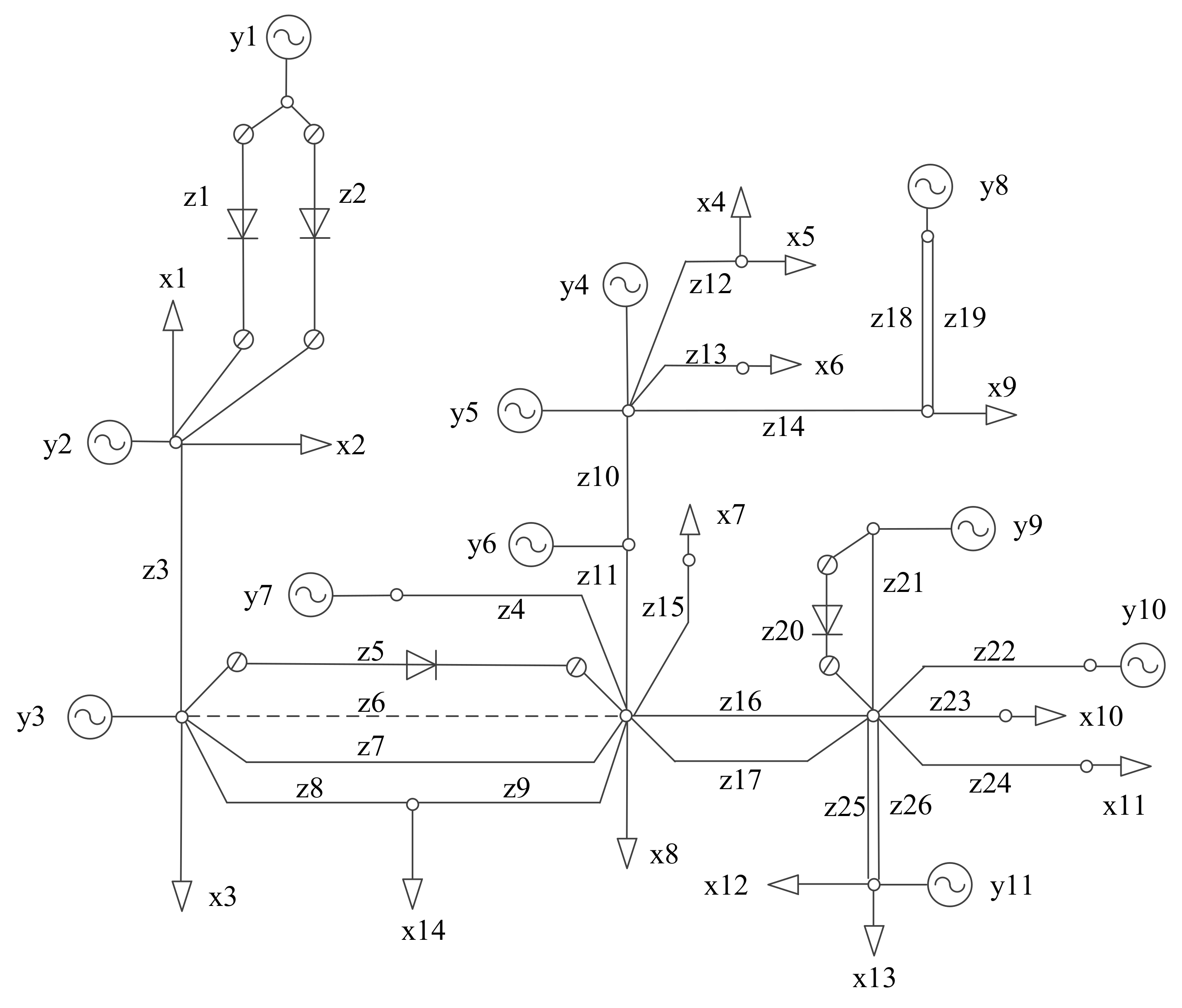
5.2. 29-Bus Test System
5.3. Comparison and Analysis
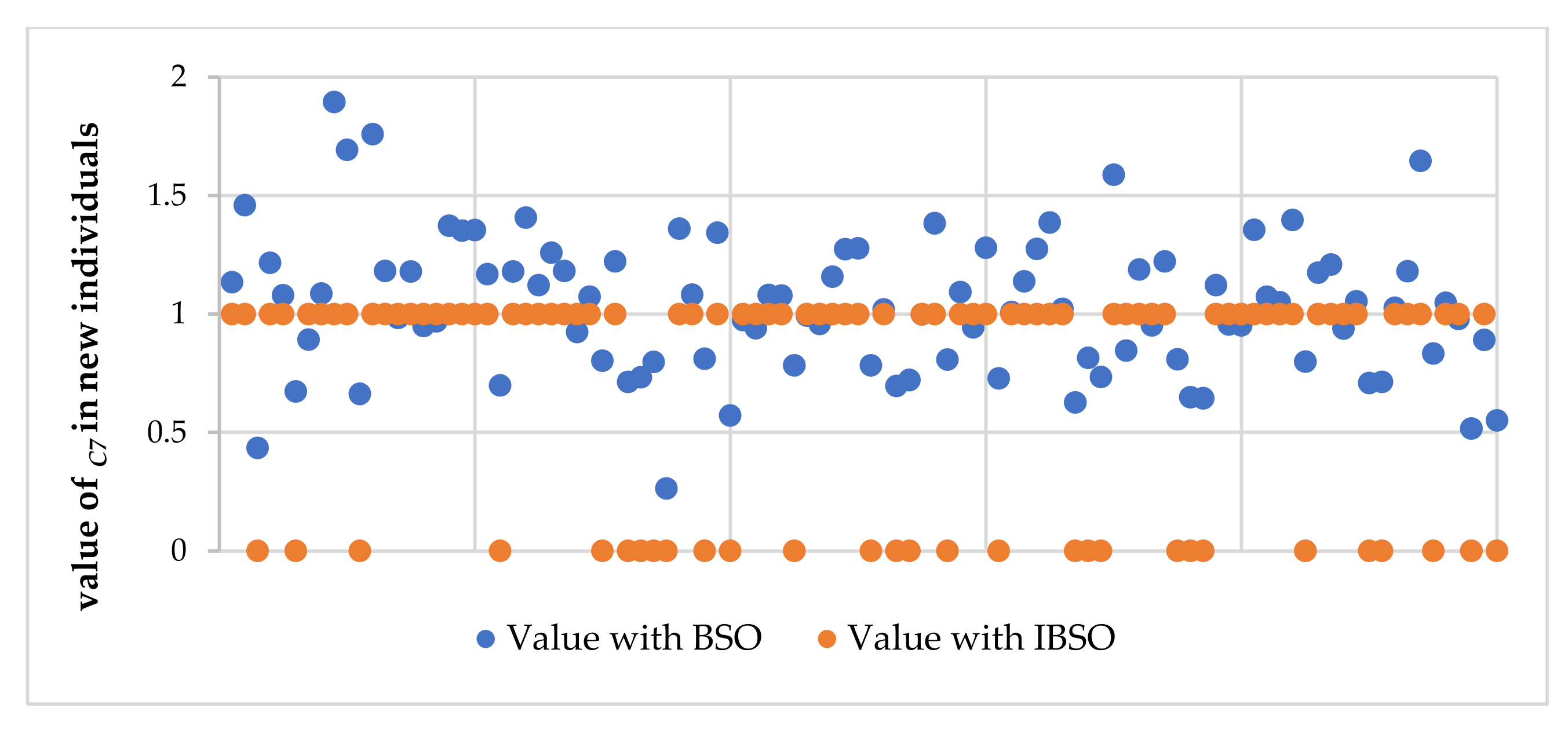
5.3.1. Comparison of IBSO and BSO
5.3.2. Comparison of Solving Process in Multiple Stages and in One Stage
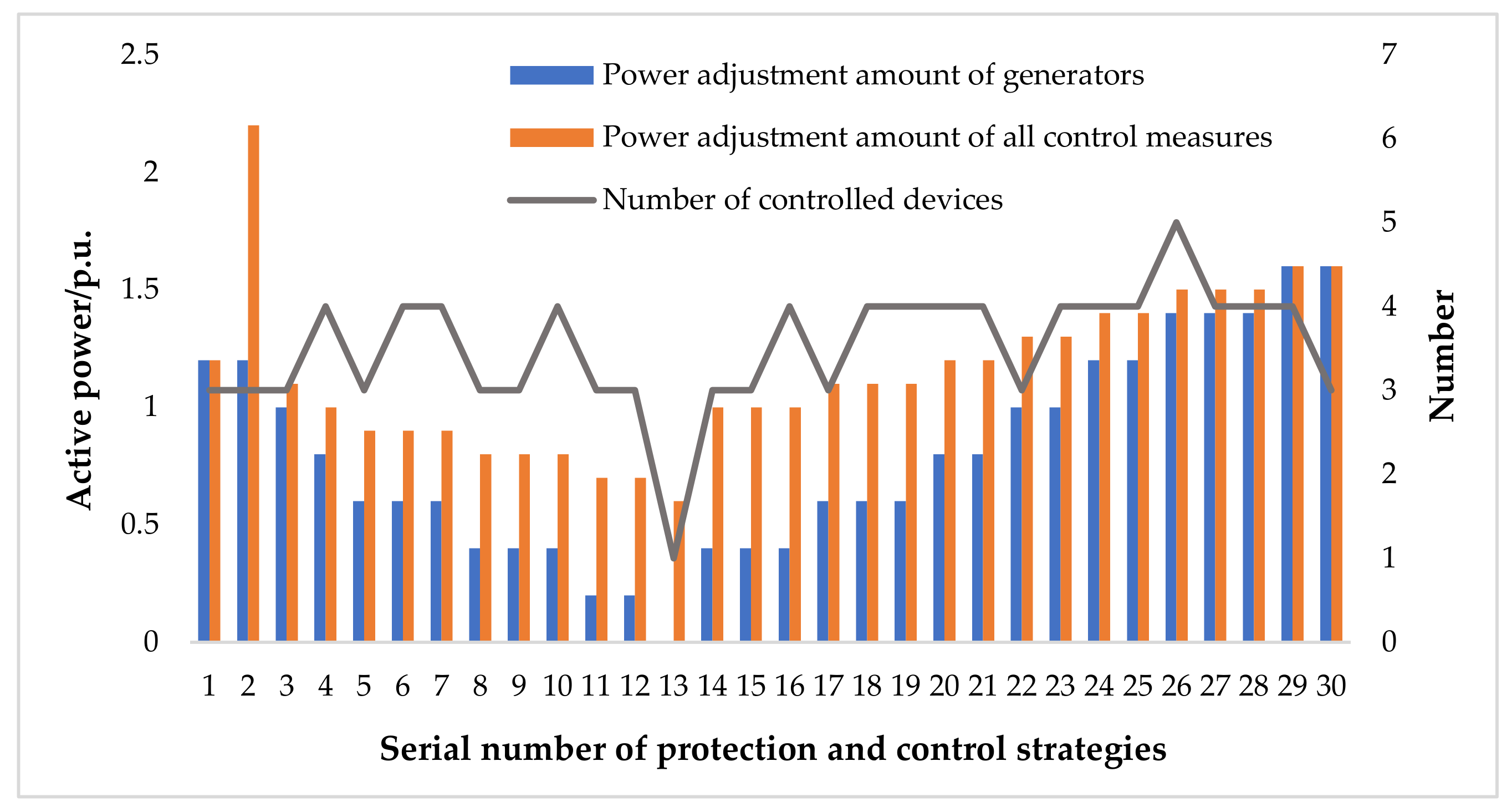
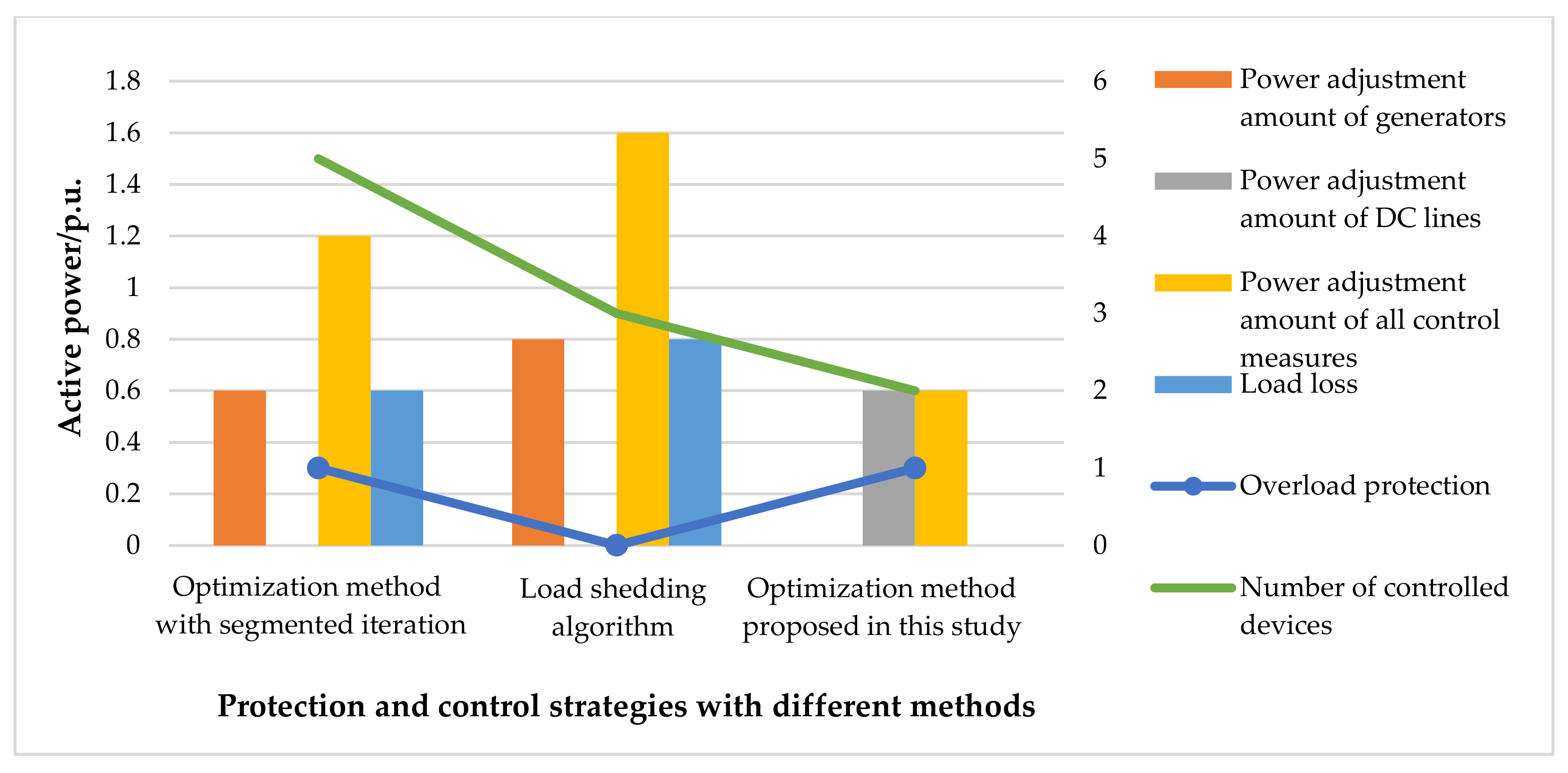
5.3.3. Comparison with Other Methods
6. Conclusions
Author Contributions
Funding
Conflicts of Interest
References
- Upama, N.; Mahshid, R.N.; Md, J.H. Interaction graphs for cascading failure analysis in power grids: A survey. Energies 2020, 13, 2219. [Google Scholar]
- Jesus, B.; Jose, M.Y. Integrated risk assessment for robustness evaluation and resilience optimisation of power systems after cascading failures. Energies 2021, 14, 2028. [Google Scholar]
- Chao, L.; Jun, Y.; Sun, Y. Risk assessment of power system considering frequency dynamics and cascading process. Energies 2018, 11, 422. [Google Scholar]
- Fan, W.; Liu, Z.; Hu, P. Cascading failure model in power grids using the complex network theory. IET Gener. Transm. Distrib. 2016, 10, 3940–3949. [Google Scholar]
- Hou, Y.; Xing, X.; Li, M.; Zeng, A.; Wang, Y. Overload cascading failure on complex networks with heterogeneous load redistribution. Physica A 2017, 481, 160–166. [Google Scholar] [CrossRef]
- Lin, X.; Yu, K.; Tong, N. Countermeasures on preventing backup protection mal-operation during load flow transferring. Int. J. Electr. Power Energy Syst. 2016, 79, 27–33. [Google Scholar] [CrossRef]
- Liu, Z.; Chen, Z.; Sun, H. Multi-agent system-based wide-area protection and control scheme against cascading events. IEEE Trans. Power Deliv. 2015, 30, 1651–1662. [Google Scholar] [CrossRef]
- Fan, J.; Mao, A.; Liu, Y.; Wu, Z.; Wang, C. Analysis of the short-time overload capability of the transmission section based on the load and ambient temperature curve. Power Syst. Prot. Control 2018, 46, 116–121. (In Chinese) [Google Scholar]
- Rios, M.A.; Kirschen, D.S.; Jayaweera, D.; Nedic, D.P.; Allan, R.N. Value of security: Modeling time-dependent phenomena and weather conditions. IEEE Trans. Power Syst. 2002, 17, 53. [Google Scholar] [CrossRef]
- Li, J.; Zhang, A.; Zhang, H.; Liu, X.; Geng, Y. Study of coordination mechanism between protection and control of regional power grid. In Proceedings of the 34th Chinese Control Conference (CCC), Hangzhou, China, 28–30 July 2015; pp. 8986–8989. [Google Scholar]
- Jiang, Y.; Chen, X.; Peng, S. Study on emergency load shedding of hybrid AC/DC receiving-end power grid with stochastic, static characteristics-dependent load model. Energies 2019, 12, 3912. [Google Scholar] [CrossRef] [Green Version]
- Majidi, M.; Aghamohammadi, M.R.; Manbachi, M. New design of intelligent load shedding algorithm based on critical line overloads to reduce network cascading failure risks. Turk. J. Electr. Eng. Comput. Sci. 2014, 22, 1395–1409. [Google Scholar] [CrossRef]
- Hu, J.; Cao, J.; Yong, T. Multi-level dispatch control architecture for power systems with demand-side resources. IET Gener. Transm. Distrib. 2015, 9, 2799–2810. [Google Scholar] [CrossRef]
- Ren, J.; Li, B.; Zhao, M.; Shi, H.; You, H.; Chen, J. Optimization for Data-Driven Preventive Control Using Model Interpretation and Augmented Dataset. Energies 2021, 14, 3430. [Google Scholar] [CrossRef]
- Laghari, J.A.; Mokhlis, H.; Bakar, A.H.A. Application of computational intelligence techniques for load shedding in power systems: A review. Energ. Convers. Manag. 2013, 75, 130–140. [Google Scholar] [CrossRef]
- Jordehi, A.R. Brainstorm optimisation algorithm (BSOA): An efficient algorithm for finding optimal location and setting of FACTS devices in electric power systems. Electr. Power Energy Syst. 2015, 69, 48–57. [Google Scholar] [CrossRef]
- Khazaei, J.; Idowu, P.; Asrari, A.; Shafaye, A.B.; Piyasinghe, L. Review of HVDC control in weak AC grids. Electr. Power Syst. Res. 2018, 162, 194–206. [Google Scholar] [CrossRef]
- Ye, P.; Yang, B.; Huang, X. Research on power flow control transformation of HVDC system through PSASP. In Proceedings of the IEEE International Conference on Energy and Environment Technology, Guilin, China, 16–18 October 2009; pp. 232–235. [Google Scholar]
- Zhu, Y.; Guo, Q.; Li, C.; Chang, D.; Chen, D.; Zhu, Y. Research on Power Modulation Strategy for MMC-HVDC and LCC-HVDC in Parallel HVDC System. In Proceedings of the IEEE 3rd Conference on Energy Internet and Energy System Integration (EI2), Changsha, China, 8–10 November 2019; pp. 1456–1461. [Google Scholar]
- Wang, J.; Liang, Z.; Xuan, X. Study on power control function for double-circuit-on-the-same-tower HVDC transmission systems. In Proceedings of the IEEE PES Asia-Pacific Power and Energy Engineering Conference (APPEEC), Hong Kong, China, 7–10 December 2014; pp. 1–5. [Google Scholar]
- Andrea, B.; Marco, I. Model Predictive Control Application for the Control of a Grid-Connected Synchronous Generator. In Proceedings of the International Electrical Engineering Congress, Krabi, Thailand, 7–9 March 2018; pp. 1–4. [Google Scholar]
- Kumars, R.; Seyed, S.H.Y.; Negin, S.M. Power flow control in multi-terminal HVDC grids using a serial-parallel DC power flow controller. IEEE Access 2018, 6, 56934–56944. [Google Scholar]
- Chen, B.; Yim, S.; Kim, H.; Kondabathini, A.; Nuqui, R. Cybersecurity of wide area monitoring, protection, and control systems for HVDC applications. IEEE Trans. Power Syst. 2021, 36, 592–602. [Google Scholar] [CrossRef]
- Zhang, Q.; Shi, Z.; Wang, Y. Security assessment and coordinated emergency control strategy for power systems with multi-infeed HVDCs. Energies 2020, 13, 3174. [Google Scholar] [CrossRef]
- Chandra, C.N.; Banerji, A.; Biswas, S.K. Survey on major blackouts analysis and prevention methodologies. In Proceedings of the Michael Faraday IET International Summit, Kolkata, India, 12–13 September 2015; pp. 297–302. [Google Scholar]
- Qi, J.; Dobson, I.; Mei, S. Towards estimating the statistics of simulated cascades of outages with branching processes. IEEE Trans. Power Syst. 2013, 28, 3410–3419. [Google Scholar] [CrossRef]
- Zhou, Z.; Wang, X.; Du, D.; Li, Y.; Li, M. A Coordination strategy between relay protection and stability control under overload conditions. Proc. CSEE 2013, 28, 146–153. (In Chinese) [Google Scholar]
- Wang, J.W.; Rong, L.L. Robustness of the Western United States power grid under edge attack strategies due to cascading failures. Safety Sci. 2011, 49, 807–812. [Google Scholar] [CrossRef]
- Bakhtyar, H.; Hadi, A.M.; Claus, L.B. Centralized load shedding based on thermal limit of transmission lines against cascading events. In Proceedings of the IEEE Power & Energy Society General Meeting, Chicago, IL, USA, 16–20 July 2017; pp. 1–5. [Google Scholar]
- Sun, M.; Min, Y.; Chen, L.; Hou, K.; Xia, D.; Mao, H. Optimal auxiliary frequency control of wind turbine generators and coordination with synchronous generators. CSEE J. Power Energy Syst. 2021, 7, 78–85. [Google Scholar]
- Islam, R.S.; Sutanto, D.; Muttaqi, K.M. A Distributed multi-agent based emergency control approach following catastrophic disturbances in interconnected power systems. IEEE Trans. Power Syst. 2016, 31, 2764–2775. [Google Scholar] [CrossRef]
- Chen, G.; Wang, Y.; Lu, G.; Hu, J.; You, D.; Zhang, F.; He, Z. An improved load-shedding model based on power flow tracing. In Proceedings of the 12th World Congress on Intelligent Control and Automation (WCICA), Guilin, China, 12–15 June 2016; pp. 1590–1593. [Google Scholar]
- Baczyńska, A.; Niewiadomski, W. Power flow tracing for active congestion management in modern power systems. Energies 2020, 13, 4860. [Google Scholar] [CrossRef]
- Niu, R.; Zeng, Y.; Cheng, M.; Wang, X. Study on load-shedding model based on improved power flow tracing method in power system risk assessment. In Proceedings of the 4th International Conference on Electric Utility Deregulation and Restructuring and Power Technologies (DRPT), Weihai, China, 6–9 July 2011; pp. 45–50. [Google Scholar]
- Subba, R.N.V.; Kesava, R.G.; Sivanagaraju, S. Power flow tracing by graph method using BFS technique. In Proceedings of the International Conference on Advances in Power Conversion and Energy Technologies (APCET), Mylavaram, India, 2–4 August 2012; pp. 1–5. [Google Scholar]
- Sobhy, M.A. Transmission loss allocation through complex power flow tracing. IEEE Trans. Power Syst. 2007, 22, 2240–2248. [Google Scholar]
- Shi, Y. Brain storm optimization algorithm. In Proceedings of the 2nd International Conference of Swarm Intelligence, Chongqing, China, 14–16 June 2011; pp. 303–309. [Google Scholar]
- Wang, Z. Research on Identification of transmission section and coordination strategy of protection and control measures with multipsource information. Doctoral Dissertation, Beijing Jiaotong University, Beijing, China, 2019. [Google Scholar]
- Wang, Z.; Li, J.; Chen, W.; Xiao, Z.; Zhang, X.; Shen, H. Coordination and optimization method of line overload protection and control measures based on subsection iteration. Electr. Power Autom. Equip. 2021, 41, 114–121. (In Chinese) [Google Scholar]
- Choi, Y.; Lim, Y.; Kim, H. Optimal load shedding for maximizing satisfaction in an islanded microgrid. Energies 2017, 10, 45. [Google Scholar] [CrossRef] [Green Version]

| Reserve | Response Time | State |
|---|---|---|
| instantaneous reserve | seconds | sync with power system |
| fast spinning reserve | 0–10 min | sync with power system |
| fast non-spinning reserve | 0–10 min | out-sync |
| thirty-minute reserve | 10–30 min | out-sync |
| sixty-minute reserve | 30–60 min | out-sync |
| cold reserve | >60 min | out-sync |
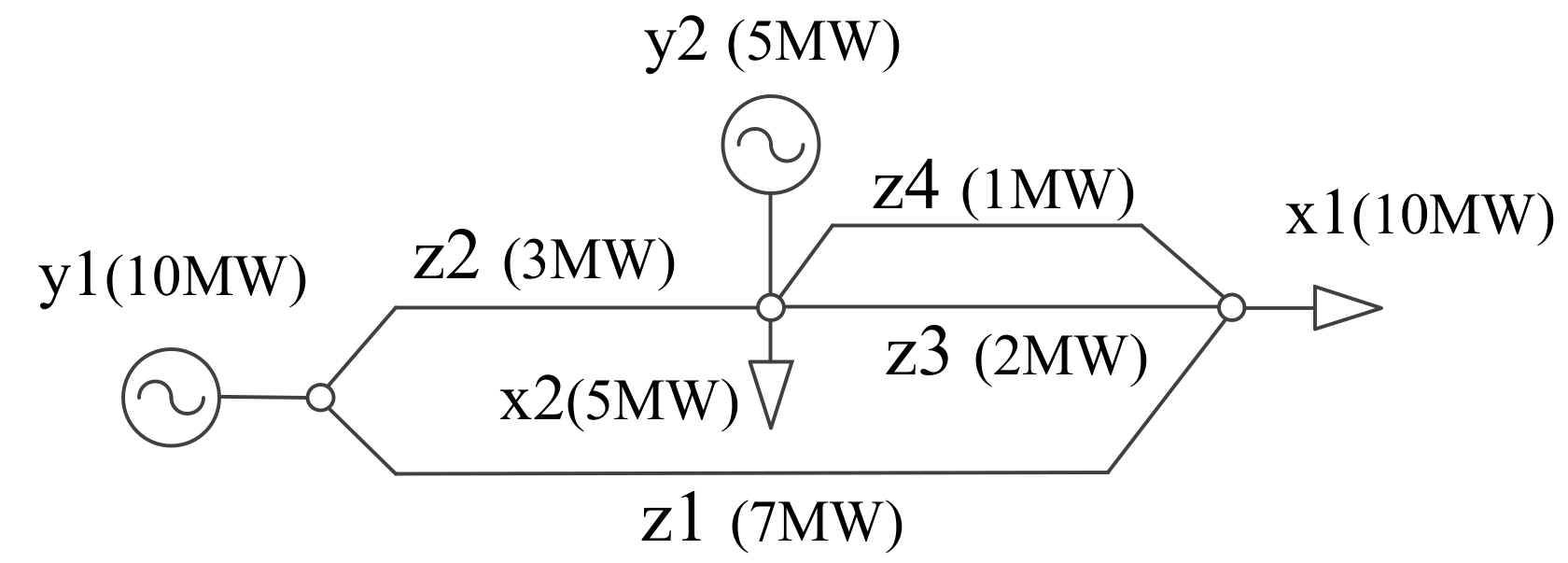
| Path | Devices | Active Power |
|---|---|---|
| 1 | y1-z1-x1 | 7 MW |
| 2 | y1-z2-z3-x1 | 0.75 MW |
| 3 | y1-z2-z4-x1 | 0.375 MW |
| 4 | y1-z2-x2 | 1.875 MW |
| 5 | y2-z3-x1 | 1.25 MW |
| 6 | y2-z4-x1 | 0.625 MW |
| 7 | y2-x2 | 3.125 MW |
| Transmission Line | Active Power (p.u.) | Transmission Capacity (p.u.) | Transmission Line | Active Power (p.u.) | Transmission Capacity (p.u.) |
|---|---|---|---|---|---|
| z1 | 6.23 | 4.92 | z5 | 3.68 | 4.42 |
| z2 | - | - | z6 | 3.39 | 4.84 |
| z3 | - | - | z7 | 3.39 | 4.84 |
| z4 | 1.30 | 1.86 | z8 | 1.41 | 2.01 |
| Generator | Initial Power (p.u.) | Power Adjustment Amount (p.u.) | Load | Initial Power (p.u.) | Power Adjustment Amount (p.u.) |
|---|---|---|---|---|---|
| y1 | 4.52 | −4.52~0 (≤5 min) −4.52~0 (≤10 min) −4.52~0 (≤30 min) | x1 | 2.72 | −2.72~0 (≤1 min) |
| y2 | 6.23 | −6.23~0, 2 (≤5 min) −6.23~0, 2, 4 (≤10 min) −6.23~0, 2, 4 (≤30 min) | x2 | 6.78 | −6.78, −3.39, 0 (≤1 min) |
| y3 | 3.21 | −3.21~0 (≤5 min) −3.21~1 (≤10 min) −3.21~1 (≤30 min) | x3 | 3.05 | −3.05, −1.5, 0 (≤1 min) |
| x4 | 1.41 | −1.41, 0 (≤1 min) |
| Path | Devices | Path | Devices | Path | Devices |
|---|---|---|---|---|---|
| 1 | y1-x1 | 8 | y2-z1-z4-z7-x2 | 15 | y3-z5-z6-x2 |
| 2 | y1-z6-x2 | 9 | y2-z1-z5-z7-x2 | 16 | y3-z4-z7-x2 |
| 3 | y1-z7-x2 | 10 | y2-z1-x3 | 17 | y3-z5-z7-x2 |
| 4 | y2-z1-z4-x1 | 11 | y2-z1-z8-x4 | 18 | y3-x3 |
| 5 | y2-z1-z5-x1 | 12 | y3-z4-x1 | 19 | y3-z8-x4 |
| 6 | y2-z1-z4-z6-x2 | 13 | y3-z5-x1 | - | - |
| 7 | y2-z1-z5-z6-x2 | 14 | y3-z4-z6-x2 | - | - |
| Transmission Line | Active Power (p.u.) | Overload | Transmission Line | Active Power (p.u.) | Overload |
|---|---|---|---|---|---|
| z1 | 4.92 | No | z5 | 3.68 | No |
| z2 | - | No | z6 | 3.39 | No |
| z3 | - | No | z7 | 3.39 | No |
| z4 | 0.99 | No | z8 | 1.41 | No |
| Transmission Line | Active Power (p.u.) | Transmission Capacity (p.u.) | Transmission Line | Active Power (p.u.) | Transmission Capacity (p.u.) |
|---|---|---|---|---|---|
| z1 | 2.00 | 2.40 | z14 | 4.20 | 5.25 |
| z2 | 2.00 | 2.40 | z15 | 1.41 | 2.01 |
| z3 | 1.30 | 1.85 | z16 | 1.41 | 2.01 |
| z4 | 4.50 | 5.63 | z17 | 0.56 | 0.80 |
| z5 | 3.00 | 3.60 | z18 | 0.56 | 0.80 |
| z6 | - | - | z19 | 1.00 | 1.20 |
| z7 | 2.80 | 2.00 | z20 | 0.55 | 0.79 |
| z8 | 2.80 | 5.00 | z21 | 2.30 | 3.29 |
| z9 | 2.00 | 2.86 | z22 | 2.20 | 3.14 |
| z10 | 1.31 | 1.87 | z23 | 1.51 | 2.16 |
| z11 | 3.50 | 5.00 | z24 | 1.48 | 2.11 |
| z12 | 2.60 | 3.71 | z25 | 1.48 | 2.11 |
| z13 | 4.62 | 5.78 | - | - | - |
| Generator | Initial Power (p.u.) | Power Adjustment Amount (p.u.) | Load | Initial Power (p.u.) | Maximum Rate for Load Shedding |
|---|---|---|---|---|---|
| y1 | 4.00 | −4, 0 | x1 | 4.00 | 100% |
| y2 | 4.80 | −4.8, −2.4, 0 | x2 | 6.10 | 100% |
| y3 | 10.20 | −10.2~0.8 | x3 | 0.80 | 100% |
| y4 | 4.00 | −4~0 | x4 | 2.50 | 100% |
| y5 | 4.72 | −4.72, 0 | x5 | 1.00 | 100% |
| y6 | 0.69 | 0.69, 0 | x6 | 2.60 | 100% |
| y7 | 4.50 | −4.50 ~ 0 | x7 | 4.20 | 100% |
| y8 | 1.12 | −1.12~0, 0.1, 0.2 | x8 | 5.58 | 100% |
| y9 | 1.55 | −1.55 ~ 0, 0.1, 0.2, 0.3 | x9 | 5.74 | 100% |
| y10 | 2.30 | −2.3~0 | x10 | 2.20 | 100% |
| y11 | 2.30 | −2.3~0, 0.5 | x11 | 1.51 | 100% |
| - | - | - | x12 | 2.26 | 100% |
| - | - | - | x13 | 3.00 | 100% |
| Transmission Line | Active Power (p.u.) | Overload | Transmission Line | Active Power (p.u.) | Overload |
|---|---|---|---|---|---|
| z1 | 2.00 | No | z14 | 4.20 | No |
| z2 | 2.00 | No | z15 | 1.41 | No |
| z3 | 1.30 | No | z16 | 1.41 | No |
| z4 | 4.50 | No | z17 | 0.56 | No |
| z5 | 3.60 | No | z18 | 0.56 | No |
| z6 | - | No | z19 | 1.00 | No |
| z7 | - | No | z20 | 0.55 | No |
| z8 | 5.00 | No | z21 | 2.30 | No |
| z9 | 2.00 | No | z22 | 2.20 | No |
| z10 | 1.31 | No | z23 | 1.51 | No |
| z11 | 3.50 | No | z24 | 1.48 | No |
| z12 | 2.60 | No | z25 | 1.48 | No |
| z13 | 4.62 | No | - | - | - |
| No. | Strategy |
|---|---|
| 1 | c7 = 1, y3↓0.6 p.u. 1, y8↑0.1 p.u. 2, y11↑0.5 p.u. |
| 2 | c7 = 1, y3↓0.6 p.u., y9↑0.1 p.u., y11↑0.5 p.u. |
| 3 | c7 = 1, z5↑0.1 p.u., y3↓0.5 p.u., y11↑0.5 p.u. |
| 4 | c7 = 1, z5↑0.2 p.u., y3↓0.4 p.u., y8↑0.2 p.u., y9↑0.2 p.u. |
| 5 | c7 = 1, z5↑0.3 p.u., y3↓0.3 p.u., y9↑0.3 p.u. |
| 6 | c7 = 1, z5↑0.3 p.u., y3↓0.3 p.u., y8↑0.1 p.u., y9↑0.2 p.u. |
| 7 | c7 = 1, z5↑0.3 p.u., y3↓0.3 p.u., y8↑0.2 p.u., y9↑0.1 p.u. |
| 8 | c7 = 1, z5↑0.4 p.u., y3↓0.2 p.u., y8↑0.2 p.u. |
| 9 | c7 = 1, z5↑0.4 p.u., y3↓0.2 p.u., y9↑0.2 p.u. |
| 10 | c7 = 1, z5↑0.4 p.u., y3↓0.2 p.u., y8↑0.1 p.u., y9↑0.1 p.u. |
| 11 | c7 = 1, z5↑0.5 p.u., y3↓0.1 p.u., y8↑0.1 p.u. |
| 12 | c7 = 1, z5↑0.5 p.u., y3↓0.1 p.u., y9↑0.1 p.u. |
| 13 | c7 = 1, z5↑0.6 p.u. |
| 14 | c7 = 0, z5↑0.6 p.u., y3↓0.2 p.u., y8↑0.2 p.u. |
| 15 | c7 = 0, z5↑0.6 p.u., y3↓0.2 p.u., y9↑0.2 p.u. |
| 16 | c7 = 0, z5↑0.6 p.u., y3↓0.2 p.u., y8↑0.1 p.u., y9↑0.1 p.u. |
| 17 | c7 = 0, z5↑0.5 p.u., y3↓0.3 p.u., y9↑0.3 p.u. |
| 18 | c7 = 0, z5↑0.5 p.u., y3↓0.3 p.u., y8↑0.1 p.u., y9↑0.2 p.u. |
| 19 | c7 = 0, z5↑0.5 p.u., y3↓0.3 p.u., y8↑0.2 p.u., y9↑0.1 p.u. |
| 20 | c7 = 0, z5↑0.4 p.u., y3↓0.4 p.u., y8↑0.2 p.u., y9↑0.2 p.u. |
| 21 | c7 = 0, z5↑0.4 p.u., y3↓0.4 p.u., y8↑0.1 p.u., y9↑0.3 p.u. |
| 22 | c7 = 0, z5↑0.3 p.u., y3↓0.5 p.u., y11↑0.5 p.u. |
| 23 | c7 = 0, z5↑0.3 p.u., y3↓0.5 p.u., y8↑0.2 p.u., y9↑0.3 p.u. |
| 24 | c7 = 0, z5↑0.2 p.u., y3↓0.6 p.u., y8↑0.1 p.u., y11↑0.5 p.u. |
| 25 | c7 = 0, z5↑0.2 p.u., y3↓0.6 p.u., y9↑0.1 p.u., y11↑0.5 p.u. |
| 26 | c7 = 0, z5↑0.1 p.u., y3↓0.7 p.u., y8↑0.1 p.u.,y9↑0.1 p.u., y11↑0.5 p.u. |
| 27 | c7 = 0, z5↑0.1 p.u., y3↓0.7 p.u., y8↑0.2 p.u., y11↑0.5 p.u. |
| 28 | c7 = 0, z5↑0.1 p.u., y3↓0.7 p.u., y9↑0.2 p.u., y11↑0.5 p.u. |
| 29 | c7 = 0, y3↓0.8 p.u., y8↑0.1 p.u., y9↑0.2 p.u., y11↑0.5 p.u. |
| 30 | c7 = 0, y3↓0.8 p.u., y9↑0.3 p.u., y11↑0.5 p.u. |
Publisher’s Note: MDPI stays neutral with regard to jurisdictional claims in published maps and institutional affiliations. |
© 2021 by the authors. Licensee MDPI, Basel, Switzerland. This article is an open access article distributed under the terms and conditions of the Creative Commons Attribution (CC BY) license (https://creativecommons.org/licenses/by/4.0/).
Share and Cite
He, J.; Han, N.; Wang, Z. Optimization Method for Multiple Measures to Mitigate Line Overloads in Power Systems. Energies 2021, 14, 6201. https://doi.org/10.3390/en14196201
He J, Han N, Wang Z. Optimization Method for Multiple Measures to Mitigate Line Overloads in Power Systems. Energies. 2021; 14(19):6201. https://doi.org/10.3390/en14196201
Chicago/Turabian StyleHe, Jinghan, Ninghui Han, and Ziqi Wang. 2021. "Optimization Method for Multiple Measures to Mitigate Line Overloads in Power Systems" Energies 14, no. 19: 6201. https://doi.org/10.3390/en14196201
APA StyleHe, J., Han, N., & Wang, Z. (2021). Optimization Method for Multiple Measures to Mitigate Line Overloads in Power Systems. Energies, 14(19), 6201. https://doi.org/10.3390/en14196201