Tides and Tidal Currents—Guidelines for Site and Energy Resource Assessment

Abstract

The main aim of this paper was to classify and to analyze the expeditious resource assessment procedure to help energy planners and system designers dealing with tides and tidal currents. Depending on the geographical features of the site to be evaluated, this paper reported the easiest methods to adopt for later working plans, crucial for preliminary considerations but to be supported by in situ measurements and by a more complex and detailed modelling. While tide trends are predictable by using Laplace equations and Fourier series, tidal currents velocities prediction is not easy, requiring suitable methods or hydraulic applications. Natural and artificial sites were analyzed and the best method for each type of them was presented. The latter together highlighting the minimum set of required information was discussed and provided as a toolkit for assessing tides and tidal current energy potential.

1. Introduction

Decarbonization strategies are directly promoting renewable energy sources (RES) exploitation to replace the current fossil fuel supply [1]. RES potential assessment becomes the first step of analysis and its data accuracy plays a primary role in go/no go investment decision making [2]. Several methods are available for solar and wind energy, while for marine resources, few tools or atlases [3] are available for preliminary studies.

Marine energy forms are multiple, including (i) mechanical ones such as tides, currents, and waves, (ii) chemical ones such as salinity gradients, or (iii) thermal ones such as constant heat sinks.

Among them, tidal energy can be considered predictable over a long time scale since it comes from the conversion of gravitational forces [4]. Its intermittency affects the design of the harvester, but not its reliability since accurate predictions are linked to its nature. However, its main drawback is the distribution over large surfaces entailing large efforts to exploit it. Furthermore, the electricity generated by tidal energy conversion is not steady and is not able to fill in the consumption peak of an energy system.

Tidal energy can be exploited in two main ways: (i) harvesting its height range in natural bays and estuaries or in artificial barrages; and (ii) extracting the kinetic energy from the tidal currents across natural and artificial channels [5].

Regarding case (i), the size of the barrage is determined by the bay or estuary to build an artificial basin of water whereby, in so doing, its level increases and decreases with a different period compared with the open sea. Therefore, the hydrostatic head occurs. The energy harvesters located along the barrage extract power from the in- and out- water flows. This can be compared to a low head hydro dam [6]. The calculation, indeed, follows similarly with dedicated systems of equations.

Referring to case (ii), the tidal stream enters in a bay or a channel located between a mainland and offshore island. The most important parameter for the assessment is the maximum average power, usually assumed as the average kinetic energy flux in an undisturbed state across the most constricted channel’s cross section where the strongest currents are present. Furthermore, the installation of energy harvesters plays a crucial role since their presence affects the flow. This is the reason why it is fundamental to determine the optimal threshold between amount of power to produce and the number of turbines to install. It is possible, as discussed in [7].

In order to start an installation or tidal system, the site must first be selected. A distinction between natural and artificial sites must obviously be made. The artificial sites are concerned with the construction of dams that allow vast amounts of energy to be stored but require major civil works. Instead, natural sites are synonymous with small lagoons, estuarine canals, straits, etc.

Incredible costs are needed for artificial sites, which are put towards other uses, such as environmental conservation, water storage, and viability, and not just to produce energy. The classic realization is a tidal barrage that, due to tidal forces, is a structure similar to a dam used to absorb energy from water moving in bidirectional way (inbound or outbound) through bays or rivers. A tidal barrage permits water to flood into a bay or river in the course of high tide, rather than damming water on one side like a traditional dam, and discharges the water during low tide. That is achieved at crucial times of the tidal cycle by calculating the tidal stream and regulating opening and closure of the sluice gates. In order to absorb the energy as water flows in and out, turbines are located at these sluices. The barrage technology of tidal energy exploitation requires the construction of a barrage across a bay or river where tidal currents flow. Turbines mounted in the barrage generate electricity while water flows in and out of the enclosed estuary basin, bay, or river. These systems are comparable to a hydro dam generating pressure energy due to the difference in height (head). The turbines are able to generate power when the water level outside the basin or lagoon varies relative to the water level within. Several kind of turbines could be used depending on the head and flow available, in some cases even reversible pumps or pumps as turbines [8].

Embankments, caissons, pumps, sluices, and ship locks are the essential elements of a barrage. These elements are located in very large concrete blocks.

Barrage systems depend on the high cost of civil infrastructure associated with the placement of a dam across estuarine systems. Because of the detrimental consequences associated with altering a big ecosystem where many varieties of species live, people have resisted barrages [9].

Tidal currents are more attractive for minor costs than less invasive applications [10], allowing installations in channels between an offshore island and the mainland or in a strait at the entrance to the bay. In this case, prior to making the decision, many parameters have to be considered or evaluated [11].

With the aim is to provide available power over a valuable period of time, the current velocity characterization in terms of spatio-temporal variance is needed for the siting activities: the optimum range is indicated as 1.5–3.5 m/s [12].

For designing the structural loading and power capability of the system, these parameters are inevitable. The geology of the seabed affects the construction of a kinetic energy system significantly. Recent sediment dynamics research has postulated a threshold value for initial particle movement [13,14,15]. However, bottom friction relies on various settings and forcings, including the structure of bed-sediments and sea bottom morphology [16] and the effect of hydro-dynamic processes, such as wave interaction and current bottom-boundary layers [17].

This is vital for determining whether the sediments removed will impact turbine components such as blades and structural parts under critical conditions. In addition, shore and bed-boundary layer effects and roughness have not always been taken into account, though tide trend is often the object of the theoretical output of energy.

All these parameters should be taken into account in the complete feasibility analysis of the production plant layout [18], starting from the tide oscillations, which are well-known for each site as the sum of the harmonic components, up to the geomorphology of the site, determining the flow velocity losses and thus the energy generated, and also the availability of the installation. A shore must be able to bear heavy concrete structures to decrease erosion due to sedimented currents, or simply to be defined as low roughness for retaining structures such as gravity-based structures (GBS).

In order to properly deploy the machine in a location, many details are required at this point. In particular:

• Geomorphology of the section for the optimum velocity range and bathymetry for position definition;
• The real flow field in terms of velocity intensity and frequency for each velocity over a date span;
• Planned energy output over the course of a year in order to test the installation strategy (i.e., one large or many smaller machines, depending on the previous data acquired);
• Seabed or shore, for the final design choices to mount the mooring fixtures;
• Limitations and availability of sites to be assessed for the host country’s environmental and economic effects.

Finally, once the above parameters have been established, the machine’s location and design can be considered to be almost ready in terms of feasibility.

The review articles available in the literature deal with the status of research [19] or regional outlook, such as the Ireland case [20], but a comprehensive and critical analysis of expeditious assessment methods is not available, despite the recent availability of marine databases [21].

Finally, the novelty of this paper is to provide readers an overview of the methods and analyses present in the literature for assessing the tides oscillations and, particularly, the tidal current velocities, by including, according to the sites conformation, 1D, 2D, and 3D approaches.

The main objective of this study was to help energy planners and system designers in resource assessment procedures for tides and tidal currents.

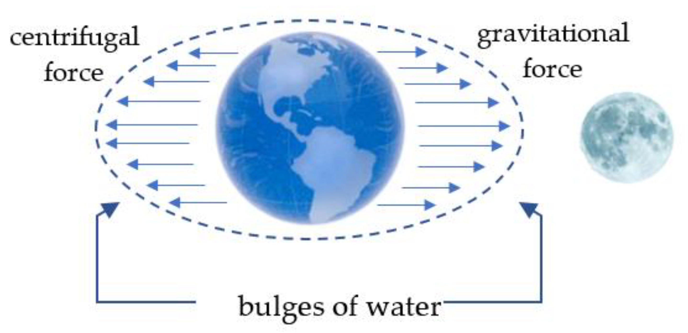
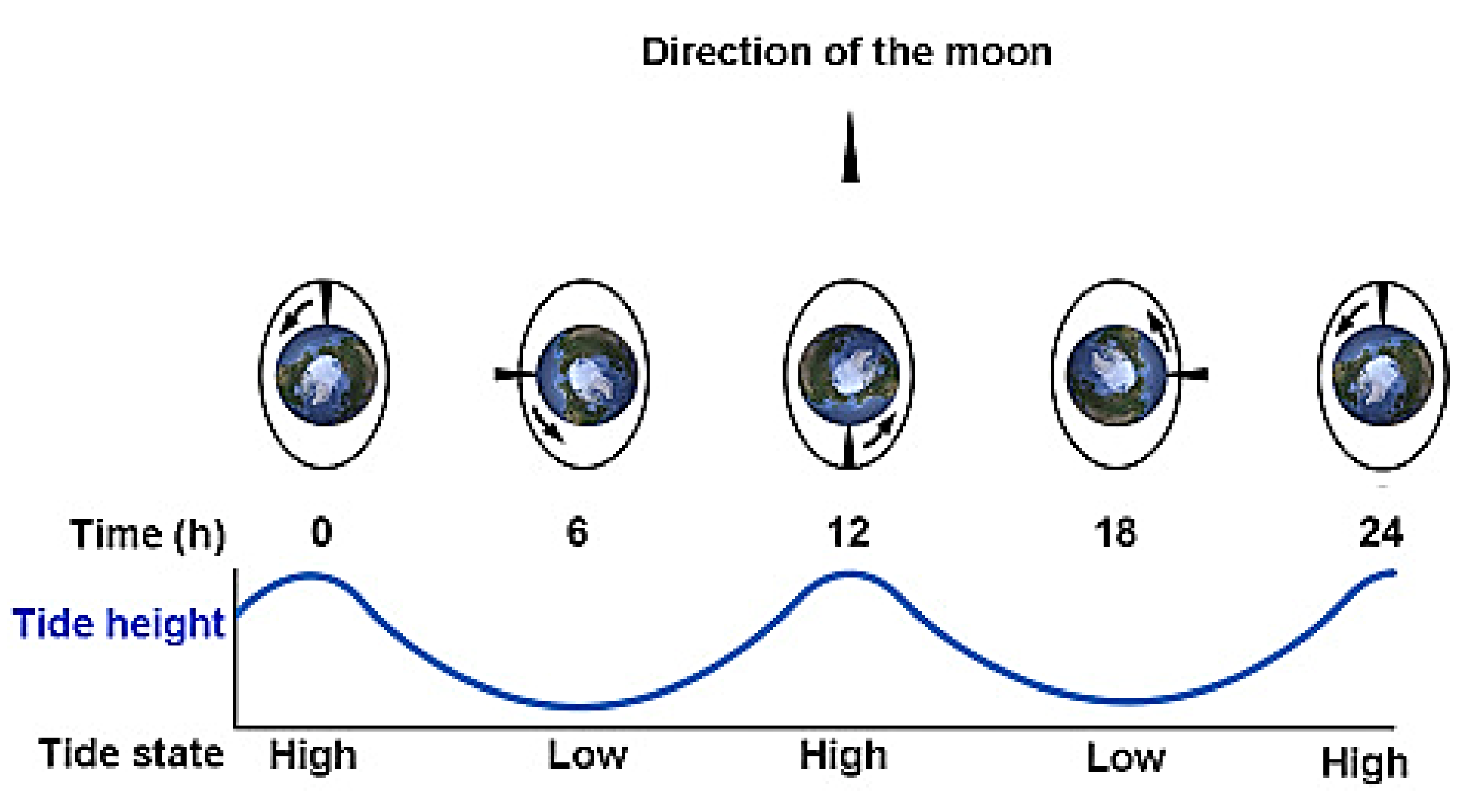
2. Material and Method—Tides Genesis: Prediction Models

Tidal energy is generated directly from the gravitational and centrifugal forces between the earth, the sun, and the moon [22]. Because of the gravitational force of the moon, the sun, and the earth and the centrifugal one produced by the mutual rotation of the earth and moon [23], a tide results in an oscillation of the ocean’s surface.

The moon exercises a gravitational force twice as big as that of the sun because it is closer to the earth. Every 24 h, 50 min, and 28 s, the tidal phenomenon occurs twice [24]. A bulge of water is formed by the gravitational force of the moon, which is stronger on the side of the earth nearest the moon. The rotation of the earth-moon system, creating a centrifugal force, creates another water bulge furthest from the moon on the side of the earth, shown in Figure 1.

The water around the landmass is at high tide when a landmass matches up with this earth-moon system. In addition, the water around it is at low tide while the landmass is at 90° to the earth-moon system (see Figure 2). Every landmass is therefore subjected to two high tides and two low tides during each cycle of the earth’s rotation [25].

The timing of these tides changes at every point on the planet as the moon rotates around the earth, and the same apex of high or low tide occurs at the same point roughly 50 min later per day [26]. Every 29.5 days, known as the lunar cycle, the moon orbits the earth. Between spring tides and neap tides, tides vary in size.

When the sun and moon are aligned with the earth, spring tides occur, whether moving on the same side of the earth or on opposite sides, resulting in extremely high spring tides. If the sun and moon are at 90° to each other, neap tides occur, resulting in low neap tides (see Figure 3).

In particular land conformations like harbors, estuaries, and bays, the level oscillation of the ocean water also produces a horizontal movement of the water which causes tidal currents. In general, a current can flow from the oceans into the harbors, bays, and estuaries as the range of tides increase; this is called a “flood current”.

A current can flow into the oceans as the tides fall; this is called an “ebb current”. When the tide stops to act, no horizontal motion is observed; this is referred to as “slack water”.

To presume a correlation between the times of high/low tides and the times of maximum and minimum tidal currents, a ‘rule of thumb’ is adopted by many technical users of the sector. This rule implies that the flood and ebb current will occur between the high and low tides, while the periods of slack water will happen at the same time as the high and low tides. However, for most places, this rule does not apply. It is not a clear relation between the times of high/low tide and the times of slack water or maximum current. Three “base case” requirements exist. A “standing wave” form of current is the first. The cycles of slack water would be exactly the same as the high and low tides in a standing wave, with the highest flood and ebb current occurring halfway between the high and low tides.

The second is the presence of a “progressive wave”. The maximum flood and ebb would arise at the times of the high and low tides in a progressive wave, with the slack water between the times of high and low tides. The two abovementioned occurrences are illustrated in Figure 4.

A “hydraulic current” is the third case. In a hydraulic current, the current is formed at two locations joined by a waterway by the difference in height of the tides. When the difference between the two heights is the highest, the current is at its full flood or ebb. When the height of the tide at the two places is about the same, slack water occurs.

At a small number of sites, hydraulic currents exist. Some instances would be:

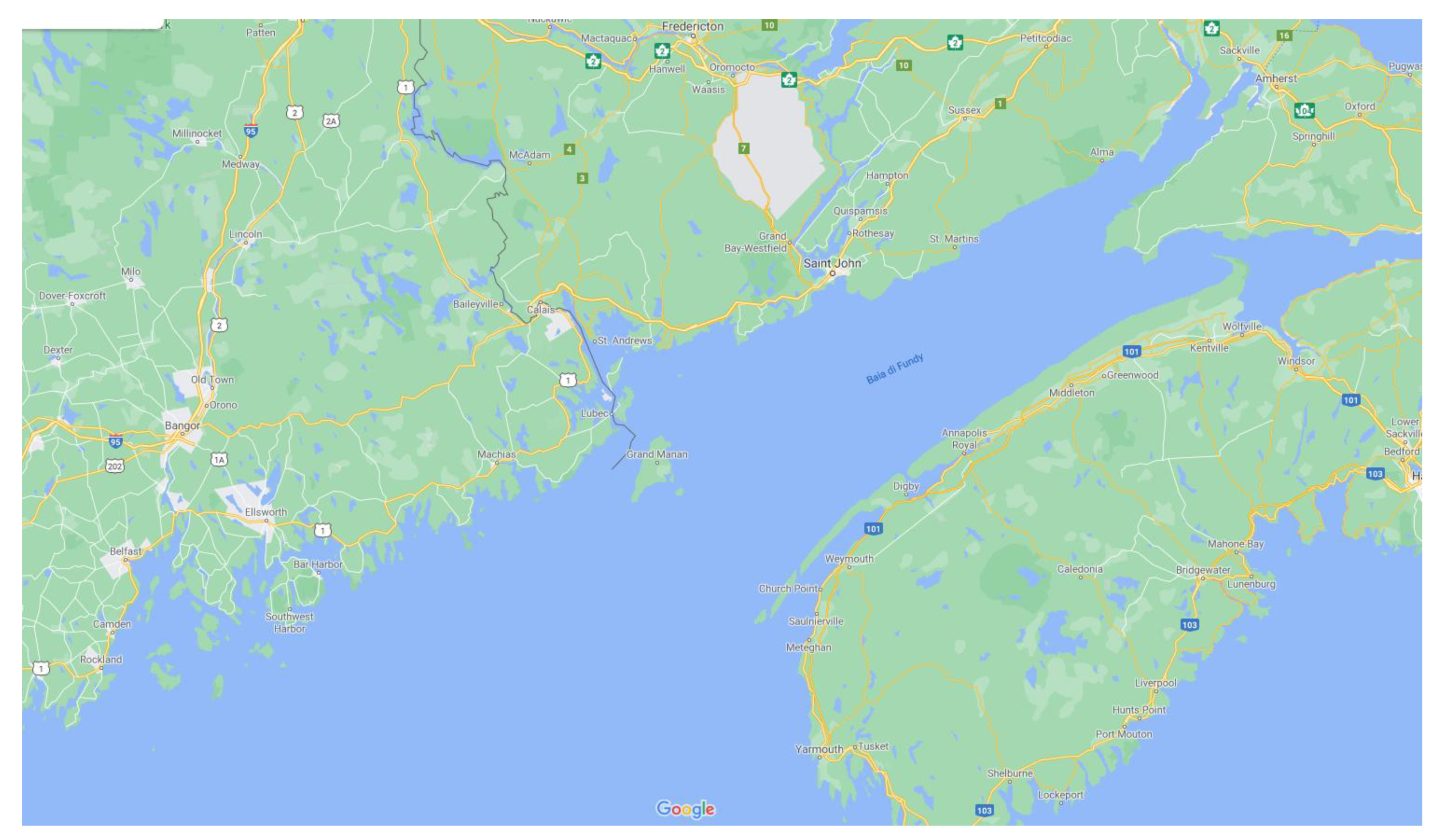
• New York’s East Channel, which ties Long Island Sound to New York Harbor;
• Any Intra Coastal Water Way parts (ICWW);
• The Canal of Chesapeake and Delaware, linking Chesapeake Bay and Delaware Bay;
• Between barrier islands that create various tidal conditions on opposite sides of the island.

Most generally, progressive currents characterize the oceanic entry of several bays and harbors. At the head of larger bays and harbors (see example in Figure 5), stationary wave conditions are most typical. Somewhere, most areas of the coast will fall in between a progressive and standing wave current.

The exact relationship between high and low tide times and maximum current or slack water is unique to each location and a general “rule of thumb” cannot be applied.

As the tidal currents are caused by the same forces that cause the tides, it is possible to predict the currents in a very similar way to the tides.

Using the same techniques used to analyze tides, observational data on the currents at a site can be evaluated and the results of such a study can be used to produce forecasts of tidal currents. However, tide predictions and tidal current predictions are performed separately because the relationship between tides and tidal currents is unique to each region.

• The times and heights of the tides are given by tide forecasts.
• The dates and speeds of maximum current and times of slack water are given by tidal current predictions.

It is up to the users to ensure that the right form of forecasts are used for their operations.

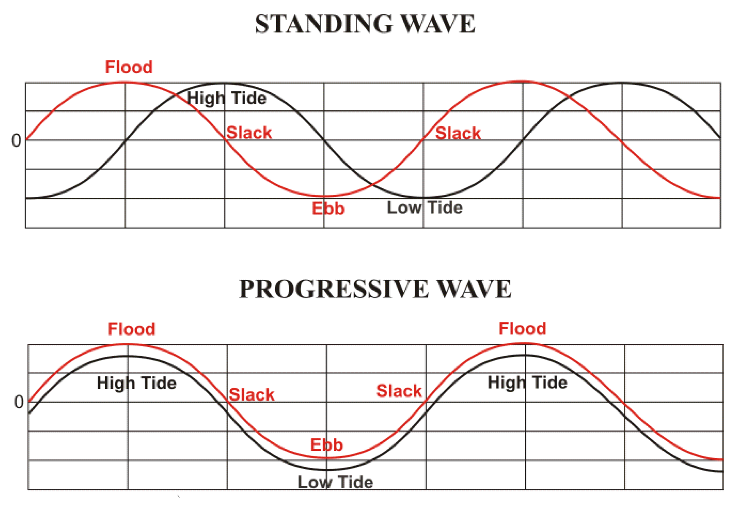
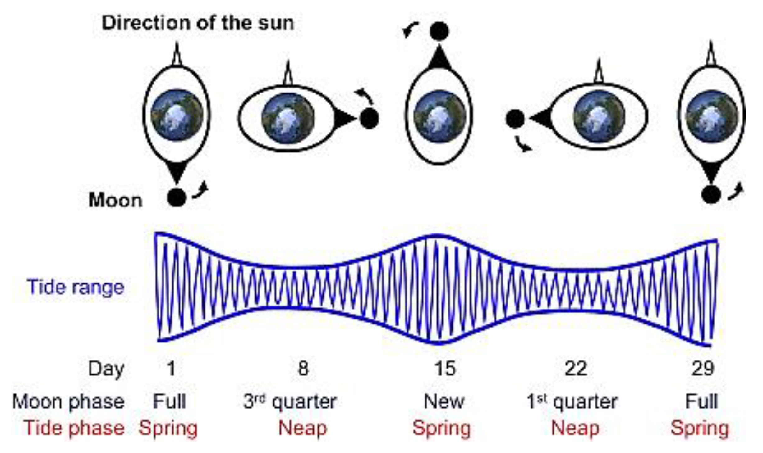
Tidal Analysis and Prediction-Tidal Constituents

Tides are completely predictable, as the number of harmonic elements can be foreseen. Approximately 62 constituents [27] are of sufficient size to be considered for potential use in the prediction of marine tides, although far fewer can often predict tides with useful precision.

Generally, seven different harmonic components cause about 83% of the variation in tides. These components originate from the influence of the moon or sun and the relative periods occur once or twice per day. For example, the so-called ‘M2’ component is typically the dominant tidal wave caused by the moon, twice daily. The periods of tidal components are constant across locations, but the relative strengths (amplitudes) vary considerably.

These major tidal constituents, determined by geographic coordinates [28] and which allow for prediction of the water level by harmonic analysis, are listed in

Table 1. Main tidal constituents with relative strength.

Symbol	Name	Period (hrs)	Strength (M2 = 1.0)
M2	Principal lunar	12.42	1.0000
S2	Principal solar	12.00	0.4652
N2	Larger lunar elliptic	12.66	0.1915
K2	Luni-solar declinational	11.97	0.0402
K1	Luni-solar declinational	23.93	0.1852
O1	Larger lunar declinational	25.82	0.4151
P1	Larger solar declinational	24.07	0.1932

together with their period and related strength.

Then, in addition to the mean sea level H_m, it is possible to reconstruct the tide height pattern as follows by considering n constituents and the corresponding frequencies ω_i and phases φ_i.

$$h(t)=H_m+{\displaystyle {\sum }_1^n{H}_{i}sin\left({\omega }_{i}t+{\varphi }_i\right)}$$

(1)

The tidal components can be produced using the global inverse solution TOPEX/Poseidon TPXO developed by Oregon State University [29]. The TPXO is a collection of global ocean tide models that best match the Laplace Tidal Equations and altimetry data in the least-square sense.

For eight primaries (i.e., M2, S2, N2, K2, K1, O1, P1, and Q1), two long periods (i.e., Mf, Mm) and three non-linear harmonic constituents (i.e., M4, MS4, MN4), on a 1440 × 721, 1/4 degree resolution complete global grid, the model considered tides as complex amplitudes of earth-relative sea-surface elevation.

If a power plant installation is considered in a natural site where tidal currents generate, like a channel, a river, an estuary, a fjord, or a strait, where more consistent tidal currents arise and flow parallel to the coast, it is necessary to know the tidal current velocities trend in order to assess the feasibility of the installation. Therefore, measurement surveys are essential. Velocity and tidal level data can be measured using an Acoustic Doppler Current Profiler (ADCP) sensor and with a built-in pressure sensor.

However, since these surveys are both expensive and time-consuming, and because of the various areas with potential suitability for tidal energy extraction, preliminary estimations require simpler, more generalized methods. A simple model would need only publicly accessible data, such as changes in sea level elevation (see Equation (1)).

3. Tides Applications and Tidal Currents Genesis: Prediction Models

In this section, both tides and tidal currents are analyzed in order to detect possible applications and assess the energy annual yield. We start from the case of a basin with barrage, which directly exploits the potential energy linked to the tides, and try to find valid correlations regarding the tidal currents, which generate from the tides themselves.

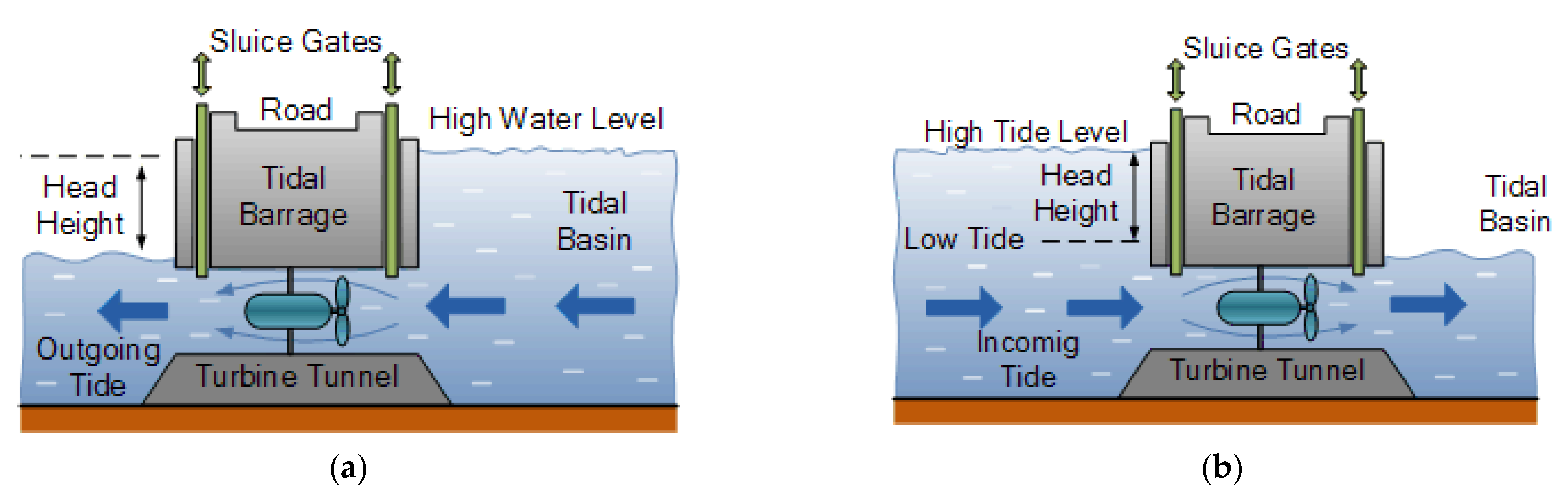
3.1. Basin with Barrage

Tidal barrages take advantage of the potential energy contained in the tides. Electricity is produced just like a hydroelectric dam with the exception that tidal currents flow in both directions, as opposed to only one direction for a dam [30].

From the tide coming in (flood tide) and out (ebb tide), a head difference is created; if the head difference is of a sufficient size, sluice gates are opened and water flows through the barrage turbines. Below, the two operating modes are explained in more detail.

• Ebb generation (Figure 6a)

Through the sluices, the basin is filled until high tide flows. Then, when the tide reaches maximum height, sluice gates are closed. At this point there could be “extra-pumping” to further increase the level. To obtain an adequate head across the dam, the turbine gates are held closed until the sea level starts to fall. Hence, when the tide reaches minimum height, see Figure 6a, the gates are opened so that while head is sufficiently high, the turbines work. This phase lasts until the difference in height (the head) is greater than zero. The sluices are then kept opened, turbines are disconnected, and the basin is again filled. With the tides, the cycle repeats. Generation of ebb (also known as generation of outflow) takes its name because generation takes place as the tide reverts tidal direction.

• Flood generation (Figure 6b)

In this case, the achievement of the energy production happens in the opposite way. The basin is filled by using the turbines working during tide flood and when the height is maximum (see Figure 6b). This is normally much less powerful than ebb generation, since the volume of the basin charged during flood is lower than the volume obtained when ebb generation operates. In fact, this last is filled first during flood generation and even with extra water from inland rivers and extra streams connected to it via the land. Therefore, the available level difference between the basin side and the sea side of the barrage, essential for the turbine power produced, decreases faster than in ebb generation. Instead of enhancing it as in ebb generation, rivers flowing into the basin can further reduce the energy capacity. This is not, of course, a concern with the “lagoon” model without the inflow of rivers.

Figure 6. Ebb generation (a) and flood generation (b) plant scheme.

Figure 6. Ebb generation (a) and flood generation (b) plant scheme.

A first simple model to evaluate the energy production through turbines inserted in the dam is based on the emptying/filling of the reservoir surrounded by the dam itself.

Therefore, it is possible to express the level of the sea as:

$$h_1(t)=h(t)+a\sin \omega t$$

(2)

where: h(t) is the mean sea level, h₁(t) is the sea level outside the basin, h₂(t) inside the basin

By introducing a suitable discharge coefficient C_d, velocity through a turbine is:

$$V=C_d\sqrt{2g\left|h_1(t)-h_2(t)\right|}$$

(3)

The flow rate through the turbine(s), having blades area A_turbine, is instead:

$$Q=V{A}_{turbine}$$

(4)

While the differential dh, referred to a Basin area B_area, changes according to:

$$dh=\frac{Q}{B_{area}(h)}dt$$

(5)

The basin area is expected to change with h in this situation. Typically, through two experimentally determinable coefficients k₁ and k₂, linear laws will take this shift into consideration as follows:

$$B_{area}=k_{1}h(t)+k_2$$

(6)

So, the level h₂ can be found by following the next equation:

$$h_{2new}=h_{2old}\pm dh$$

(7)

Ultimately, the power provided by the turbine becomes:

$$P={\eta }_{turb}{\eta }_{tr}{\eta }_{gen}\rho g{A}_{turb}{C}_d\sqrt{2g{\left|h_1(t)-h_2(t)\right|}^3}$$

(8)

It is assumed that a transmission efficiency η_tr of 67% and a turbine η_turb and generator unit η_gen global efficiency of 60%–90% are typical values for small hydro power plants. The turbine’s efficiency η_turb varies, as the flow rate and head are not constant. A turbine is usually designed to keep the efficiency constant for different flow rates for a given operating band. The efficiency will drop rapidly, however, if it exceeds a certain condition. Kaplan turbine efficiencies start to decline at 50% of the nominal flow in traditional hydro power. In the next figure (Figure 7), this occurrence is highlighted.

This impact is even greater in a tidal barrage, as the maximum head is only reached for a limited period of time and cross-flows through the turbine tunnel are required when the system reaches a very low head (less than 10% of the maximum value). The efficiency of the turbine and generator is therefore assumed to be 90% for peak power and 70% for annual average power output. There is no consideration of additional losses due to transformation, gear boxes, or downtime.

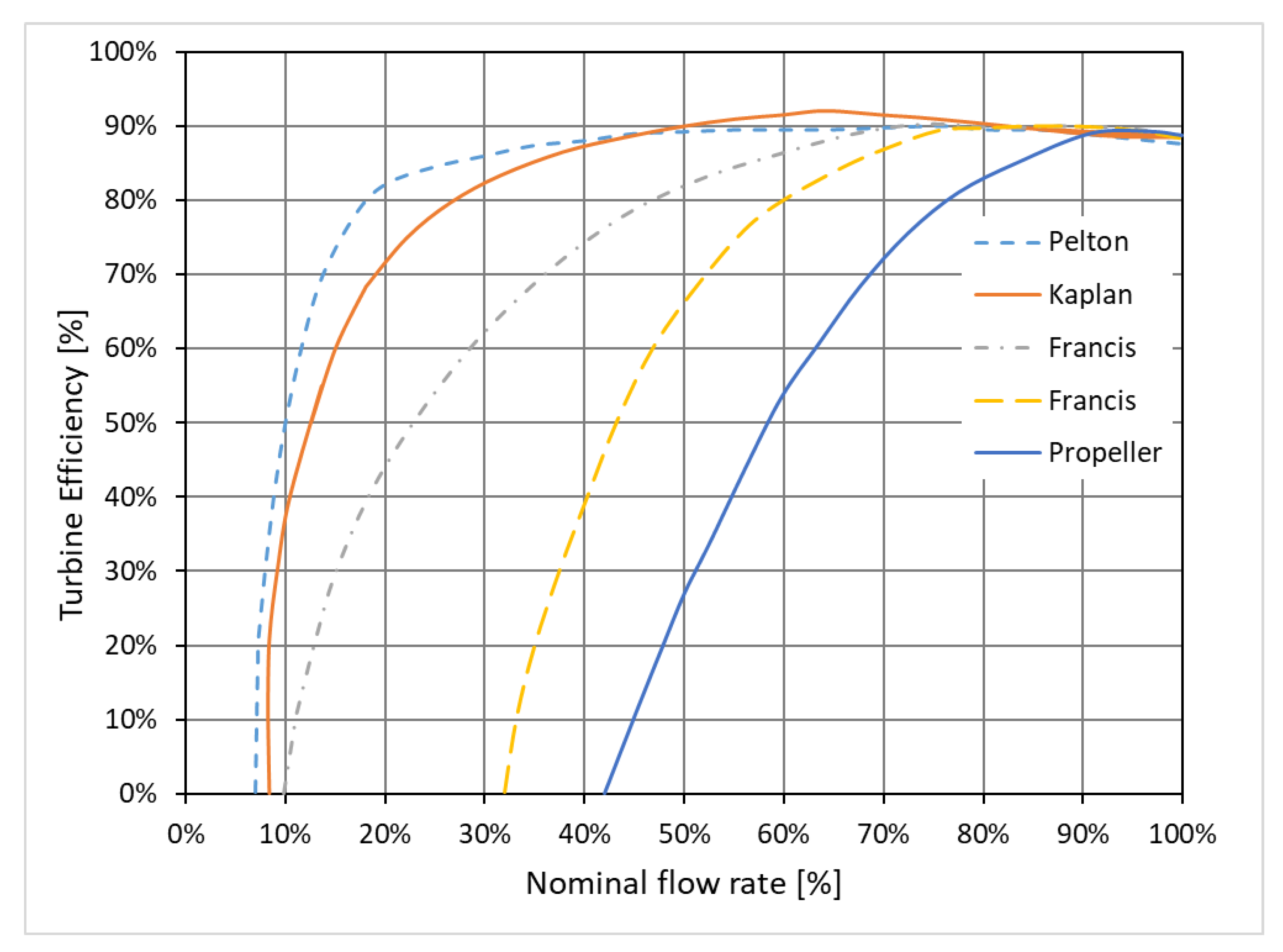
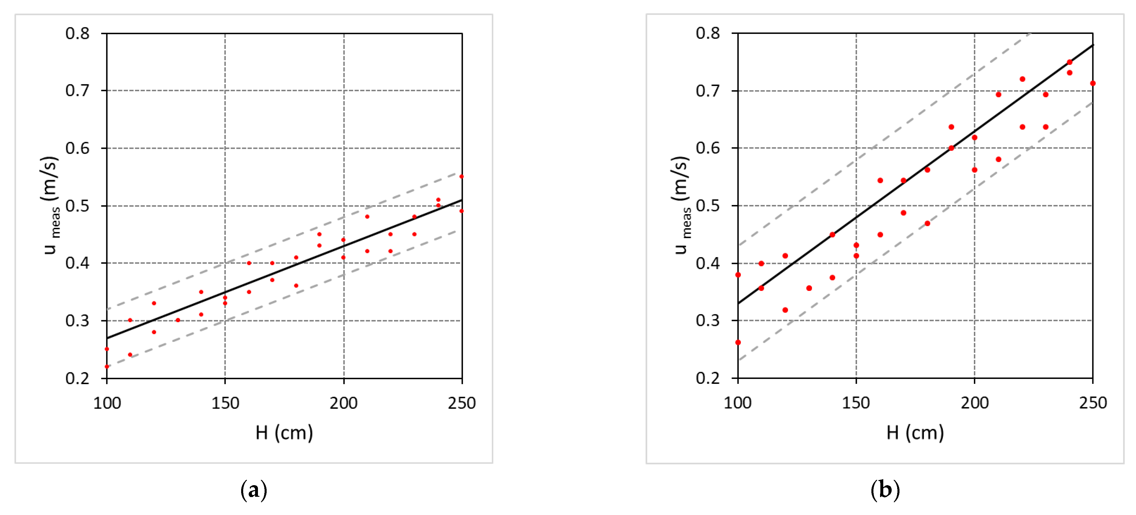
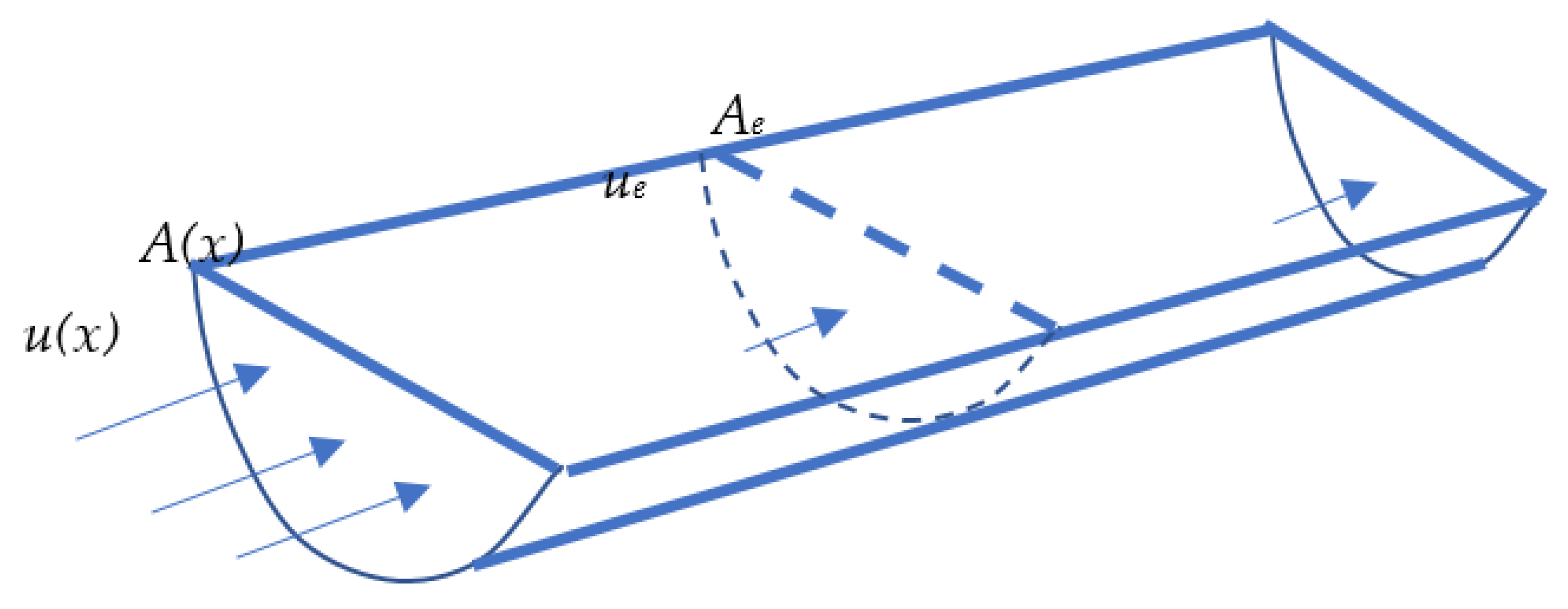
3.2. Model for Predicting Tidal Current Velocities

Tidal currents are generated from tides whenever the difference in height of the sea level is converted in flow through a wide or narrow channel, in a strait or a gorge. They flow parallel to the coast like a river and revert their direction generally twice per day. Bringing essentially kinetic energy, they can be exploited by wind turbine-like machines. Here, these machines were not analyzed, because they were not the focus of this paper. More interesting is the way to assess the trend of these currents. In this section, some models for simple evaluations are proposed, and energy resources are evaluated for both artificial sites (barrages) and natural sites (channels).

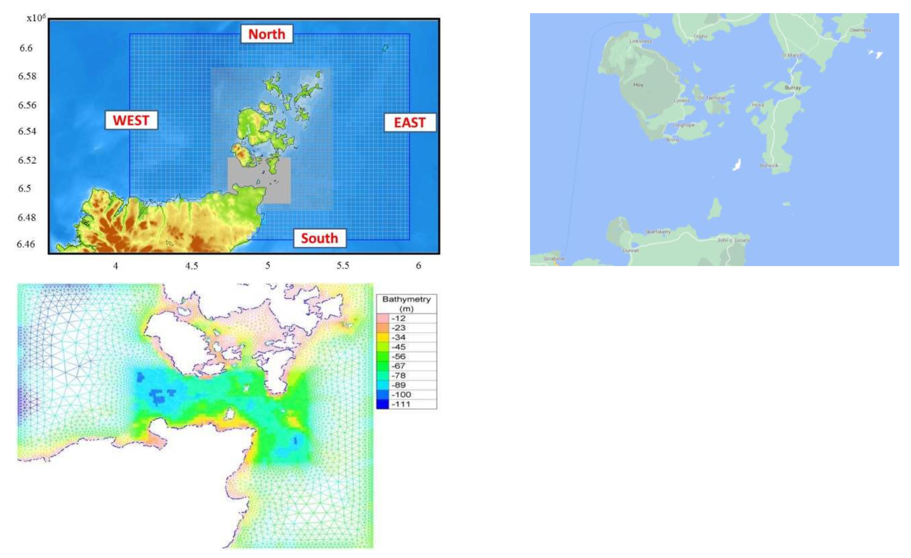
Enclosed Bay with Channel

Continuity means that the change in volume within the bay must be equal to the flow into the bay when considering an enclosed area, such as a fjord. The flow into the bay is the flow through the canal linking the bay to the open ocean and other inputs, such as discharge from the river. If one disregards the freshwater input, the continuity equation can be written as [31]:

$$A_{bay}\frac{d{h}_i}{dt}=Q$$

(9)

where A_bay is the region of the enclosed bay, which is expected not to shift with the h level in this case; h_i is the water level within the bay; and Q is the channel flow. The cumulative drop across the channel in water level is equivalent to h_o-h_i, where h_o is the level of water on the outer side of the bay in the ocean. This total water-level drop can be divided into two parts: one related to the channel friction (Δh_f) and one related to the flow acceleration towards the constriction (Δh_b).

Using the Manning number, n, the frictional resistance can be calculated according to:

$$\mathrm{\Delta }{h}_f=\frac{n^{2}L}{R^{4/3}}{\left(\frac{Q}{A_c}\right)}^2$$

(10)

where L is the channel’s length; R is the hydraulic radius; and A_c is the channel’s cross-sectional area [31]. It is possible to write the variable Δh_b as:

$$\mathrm{\Delta }{h}_b=\frac{Q^2}{2g{A}_c^2}$$

(11)

The friction and acceleration concept is assumed to be negligible in the simplest case, and Equation (9) is used to model the channel velocity.

Only continuity is applied to measure the velocity of the channel. In addition, assuming that during the tidal cycle the cross-sectional area will not change significantly, the flow will depend on the channel velocity such that Q = A_c · u. Through this, a relationship between the velocity and the tidal level can be achieved. Denoting the approximate velocity with u, the equation becomes:

$$u=\frac{A_{bay}}{A_c}\frac{d{h}_i}{dt}=\frac{A_{bay}}{A_c}\frac{d{h}_o}{dt}$$

(12)

If the tidal water level with an angular frequency of ω has a sinusoidal difference,

$$h(t)=H_{\max }\sin (\omega t)$$

(13)

The velocity is, then, u

$$u=\frac{A_{bay}}{A_c}\omega \sin \left(\omega t-\frac{\pi }{2}\right)=\frac{A_{bay}}{A_c}\omega \sin \left[\omega \left(t-\frac{T}{4}\right)\right]$$

(14)

The velocity would then have a phase shift of T/4, being T the period of the tides equal to 12 h and t the time in hours.

Equation (14) can be further extended to estimate the maximum velocity in the channel. Writing the sinusoidal variation of the velocity with u(t) = u_maxsin(ωt), the integration of Equation (12) over half a tidal period gives the maximum velocity:

$$u_{\max }=1.4\cdot {10}^{-4}\left(s^{-1}\right)\frac{A_{bay}}{A_c}{H}_{\max }$$

(15)

by considering that ω = 2π/T. i.e., 6.28/(12 × 3600) = 1.4 × 10⁻⁴.

Case study: Skarpsundet tidal channel (Norway) [31].

In the following, an example of how it is possible to estimate the tidal current velocity in a channel is reported together with ADPC measurements. The area is in the Norway fjords, and particularly the case of the Skarpsundet tidal channel is analyzed. The following figures (Figure 8a,b) report the map of the site with the channel and the connected bay highlighted.

Table 2. Values for the Skarpsundet channel.

Variable	Description	Value
ρ	Density	1025 kg/m3
L	Length of Skarpsundet	1500 m
Ac	Cross-sectional area	13,500 m2
W	Average width of channel	700 m
Hc	Average depth of Skarpsundet	15 m
Abay	Fjord Area	3.8 × 107 m2

reports useful data for applying the methodology.

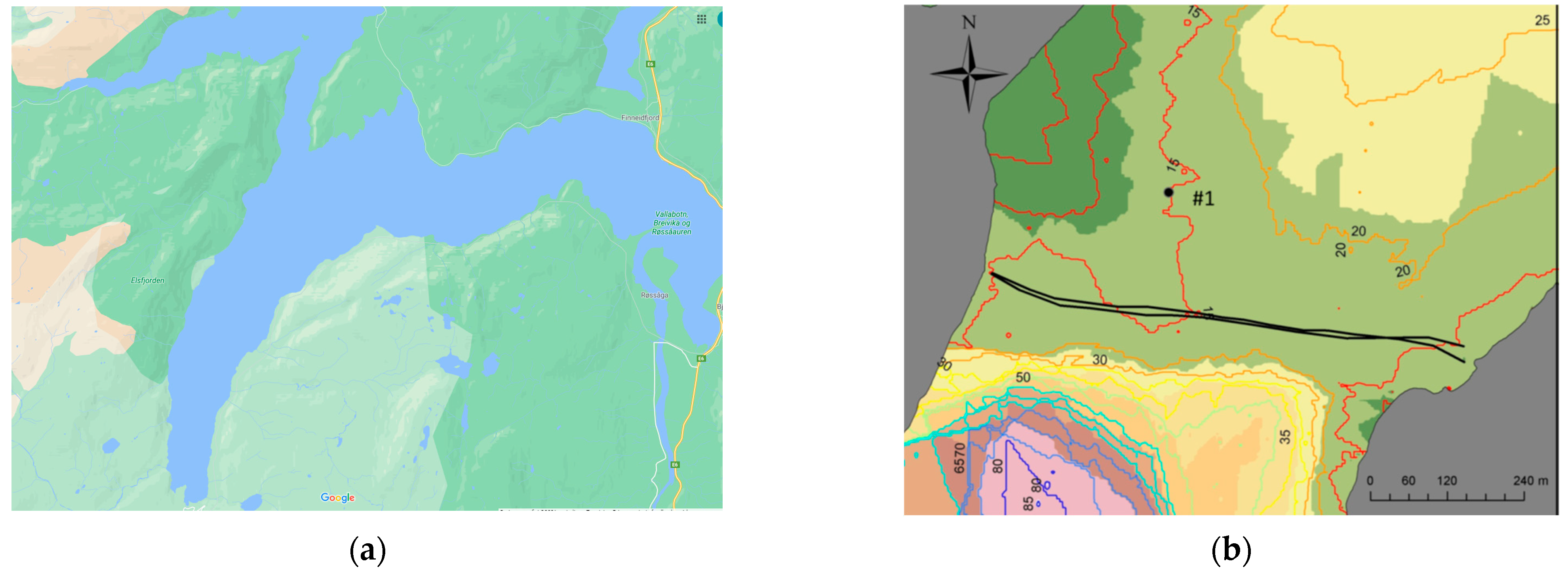
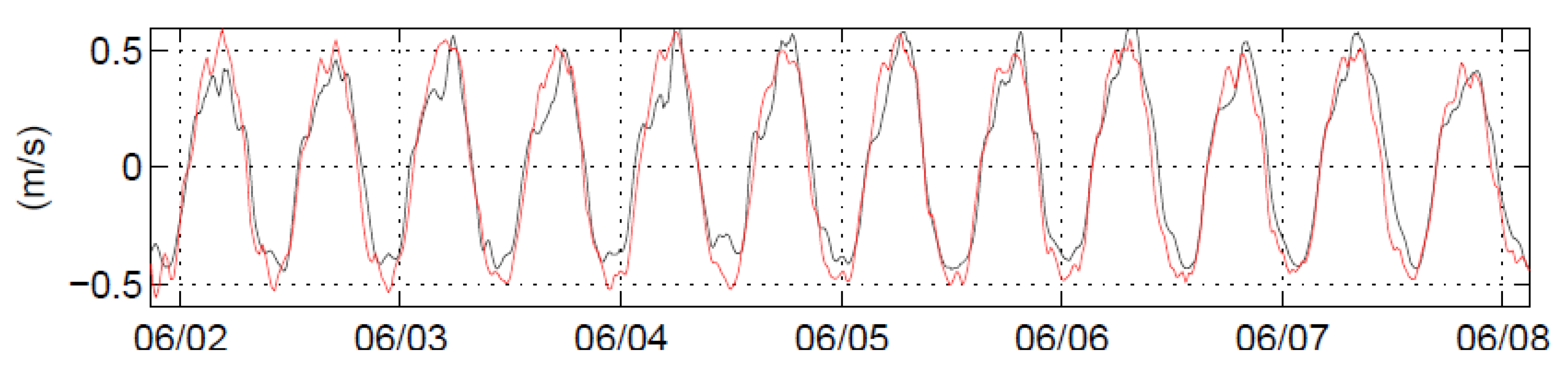
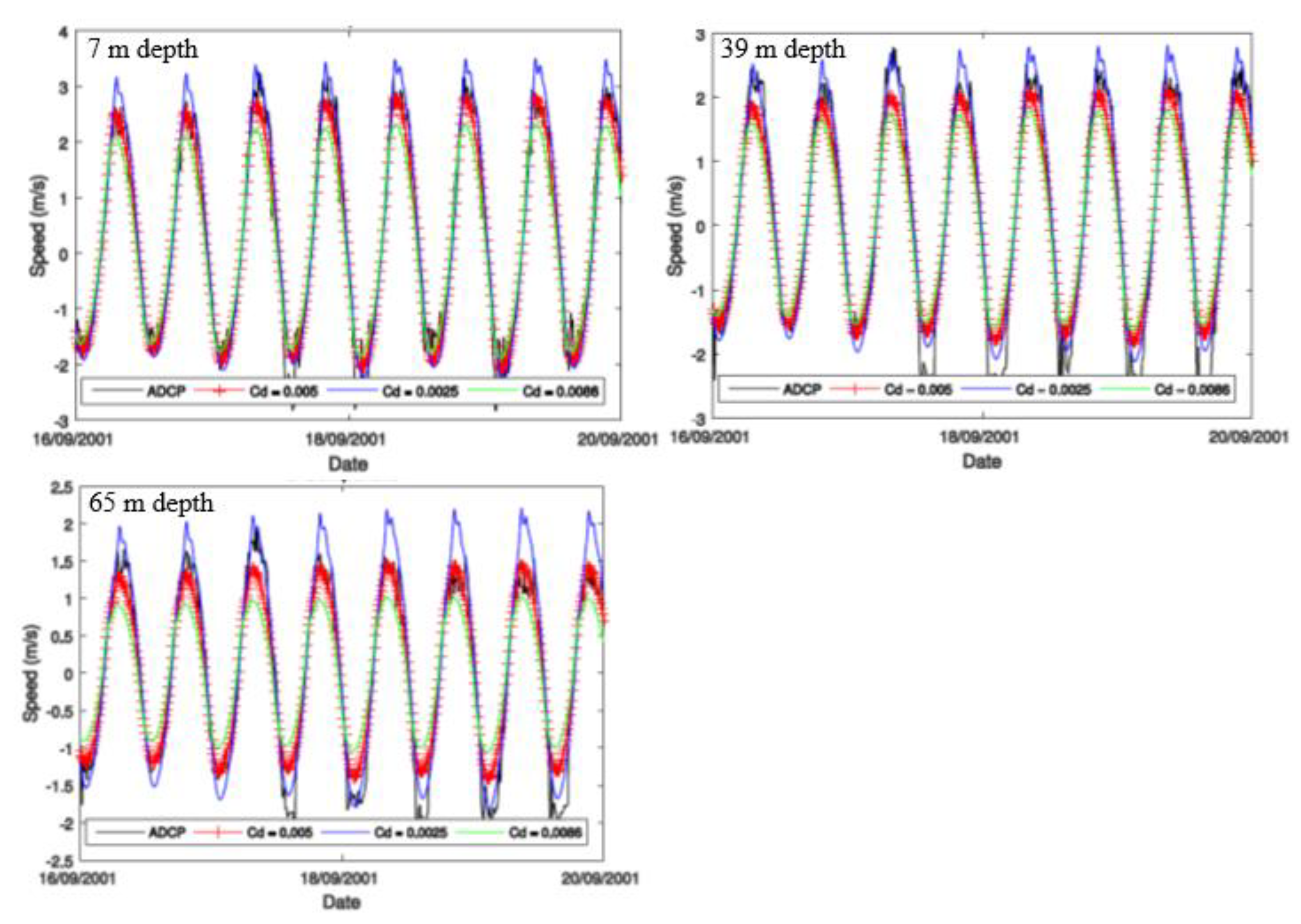
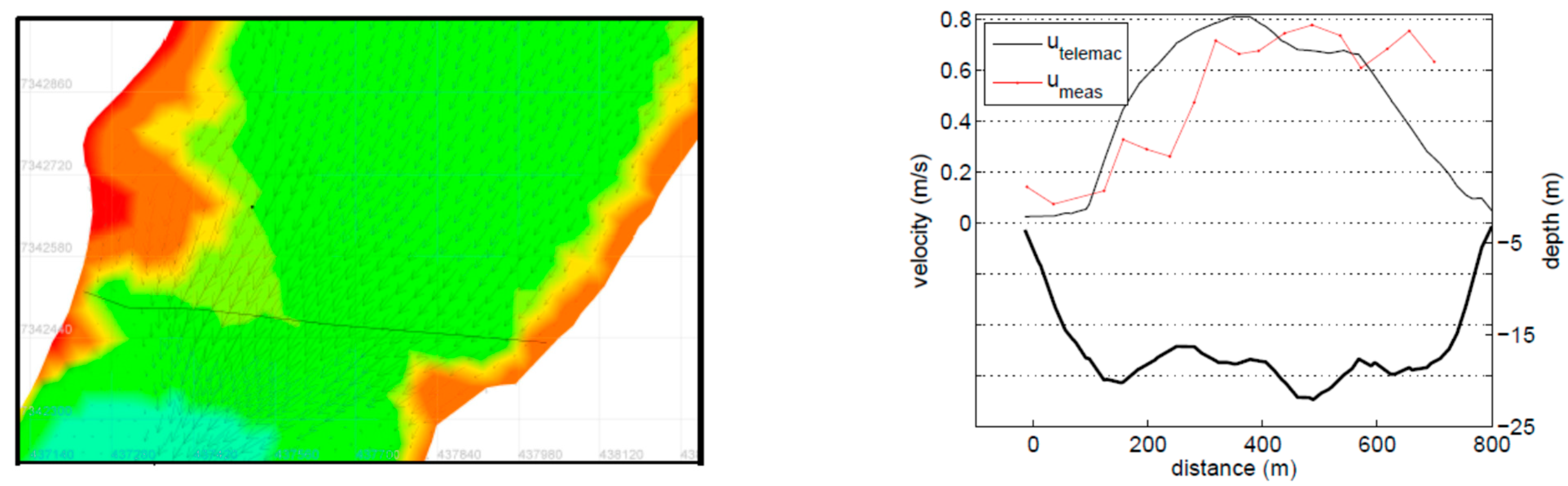
3.3. ADCP Measurements

A 600 kHz ADCP Workhorse Sentinel was used for measuring velocity and tidal level. The built-in pressure sensor of the ADCP instead was utilized for measuring the water level. By means of a downward-looking ADCP, one transect measurement and one different survey were performed. Figure 8b shows the locations of the measurements: transect measurements are marked as black lines. By using a low-frequency sampling rate, long-time measurements were performed over 43 days. The ADCP measured velocities (#1—see Figure 8b) were compared to the simulated ones obtained from TELEMAC-2D software (Figure 9). The velocity reliefs in direction North-South agreed with the simulations (Figure 9). Figure 10 illustrates the tidal velocity variations across the channel.

3.4. Maximum Velocity and Tidal Range

At this point, it is necessary to test the goodness of the methodology by verifying if the maximum velocities of the tidal range considered are according to Equation (15). On purpose, only the long-time ADCP velocity series were used by obtaining the tidal range—the difference from the maximum and minimum height or tide level—from the Norwegian Hydrographic Service (NHS). The velocities were depth averaged and smoothed over one hour, and then their maximum values, during flood and ebb, were extracted from the time series. Figure 11 highlights the results of this analysis.

The correlation plot shows that the velocity variation was stronger for the outgoing tide compared with the incoming.

$$u_{\max ,in}=0.11+0.16\cdot H$$

(16)

$$u_{\max ,out}=0.03+0.30\cdot H$$

(17)

Equations (16) and (17) are written for interpolating data measured, shown in Figure 11 together with dashed lines representing error band of ±0.05 m/s and 0.1 m/s, taking into account that H is the peak to peak difference height equal to 2H_max (see Equation (13)). It can be seen that the slope in the equation was different between the flood and the ebb tide, with a higher slope value for the ebb tide. The maximum velocity occurred, on average, 3 h and 35 min after high tide and 3 h 32 min after low tide.

Using Equation (15) and taking into account the parameters reported in Table 2, u_max became 0.4 m/s if the considered tidal range H is 200 cm. This value agrees strongly with the measured cross-sectional average velocity during flood tide (0.42 m/s—see Figure 11a), and weakly with the measured cross-sectional average velocity during ebb tide (0.63 m/s—see Figure 11b). However, measurements at a diverse location, more centered in the channel, could yield different results.

Channels

Figure 12 illustrates the stream through a variable cross-section channel. It is assumed that the current velocity u(x, t) is a function of time t and location x along the channel, but independent of the cross-channel position. The dynamic equation that governs the flow is

$$\frac{\partial u}{\partial t}+u\frac{\partial u}{\partial x}+g\frac{\partial h}{\partial x}=-F$$

(18)

Where the pressure gradient to drive the flow is given by the slope of the surface elevation h, and where F(x, t) represents an opposing force associated with natural friction and possibly turbine presence. To be independent of the cross-channel location of the frictional force associated with the turbines, the turbines must be deployed in a uniform fence across the flow, so that all the water flows through the turbines itself. If the channel is small compared with the wavelength of the tide, which usually reaches hundreds of kilometers, even in shallow water, the continuity law ensures that the flux A · u along the channel is independent of x (we neglected small changes in A associated with the rise and fall of the tide) and can be written as Q(t).

The use of this in Equation (18) and the integration along the channel means

$$c\frac{dQ}{dt}-g{h}_0\left(t\right)=-{{\displaystyle \int }}_0^{L}Fdx-\frac{1}{2}{u}_e\left|u_e\right|$$

(19)

where c is

$$c={\displaystyle \underset{0}{\overset{L}{\int }}\frac{1}{A(x)}}dx$$

(20)

The difference in sea level between the two basins is h_o(t), meaning that this difference is unaffected by the flow through the channel and also unaffected by F shifts as turbines are installed.

3.5. The Easiest Case for Tidal Currents Velocity Estimation

The natural friction and head loss associated with separation at the exit could likely to be relevant. It is assumed, however, that these effects are minimal, above all if the channel is long and wide, so that the natural regime has a balance between the difference in sea level and acceleration. Considering a sinusoidal tide:

$$h_0(t)=a\mathit{cos}(\mathit{\omega t})$$

(21)

where the amplitude is a and the frequency is ω. This forcing will, of course, at each end of the channel be the distinction of sinusoidal tides rather than reflecting forcing from only one end. By integrating Equation (18), the corresponding volume flux is

$$Q=Q_0\mathit{sin}(\mathit{\omega t})$$

(22)

$$Q_0=\frac{ga}{\omega c}$$

(23)

Taking into account the drag associated with the presence of turbines, expressed as

$${\displaystyle \underset{0}{\overset{L}{\int }}Fdx=\lambda Q}$$

(24)

Equation (19) becomes:

$$c\frac{dQ}{dt}-ga\cos \omega t=-\lambda Q$$

(25)

In this case

$$Q=\mathrm{Re}\left[\left(\frac{ga}{\lambda -ic\omega }\right)e^{-i\omega t}\right]$$

(26)

3.5.1. 3D and 2D Methods—Navier–Stokes Equations

When the site’s geometry is complex, for example when headlands and islets are present, the approaches described previously fail. Where the coast is indented and headlands and islets are present, this is the case for complex geometries. Therefore, depending on the characteristics of the seabed, more robust methods need to provide 2D or 3D approaches. The baroclinic Navier-Stokes equations were obtained by reducing the vertical momentum equation to the hydrostatic pressure assumption by applying the Boussinesq assumptions. The fluid was often believed in the simulation to be incompressible. The equations for continuity and momentum are given below [32]:

$$\frac{\partial h}{\partial t}+\frac{\partial \left[\left(d+h\right)U\right]}{\partial x}+\frac{\partial \left[\left(d+h\right)V\right]}{\partial y}+\frac{\partial \left[\left(d+h\right)W\right]}{\partial z}=Q$$

(27)

$$\begin{array}{ll}\frac{\partial U}{\partial t}+U\frac{\partial U}{\partial x}+V& \frac{\partial U}{\partial y}-fV\\ & =-g\frac{\partial h}{\partial x}-\frac{g}{{\rho }_o}\underset{-d}{\overset{h}{{\displaystyle \int }}}\frac{\partial {\rho }^{\prime }}{\partial x}dz+\frac{{\tau }_{sx-}{\tau }_{bx}}{{\rho }_o\left(d+h\right)}+v_h\left(\frac{{\partial }^{2}U}{\partial x^2}+\frac{{\partial }^{2}U}{\partial y^2}\right)\\ & +v_v\left(\frac{{\partial }^{2}U}{\partial z^2}\right)\end{array}$$

(28)

$$\begin{array}{ll}\frac{\partial V}{\partial t}+U\frac{\partial V}{\partial x}+V& \frac{\partial V}{\partial y}-fU\\ & =-g\frac{\partial h}{\partial y}-\frac{g}{{\rho }_o}\underset{-d}{\overset{h}{{\displaystyle \int }}}\frac{\partial {\rho }^{\prime }}{\partial y}dz+\frac{{\tau }_{sy-}{\tau }_{by}}{{\rho }_o\left(d+h\right)}+v_h\left(\frac{{\partial }^{2}V}{\partial x^2}+\frac{{\partial }^{2}V}{\partial y^2}\right)\\ & +v_v\left(\frac{{\partial }^{2}V}{\partial z^2}\right)\end{array}$$

(29)

$$\frac{\partial p}{\partial z}=-\rho g$$

(30)

$$\begin{array}{ll}\frac{\partial \left[\left(d+h\right)c\right]}{\partial t}& +\frac{\partial \left[\left(d+h\right)Uc\right]}{\partial x}+\frac{\partial \left[\left(d+h\right)Vc\right]}{\partial y}+\frac{\partial \left[\left(d+h\right)Wc\right]}{\partial z}\\ & =D_h\left(\frac{{\partial }^{2}c}{\partial x^2}+\frac{{\partial }^{2}c}{\partial y^2}\right)+D_v\left(\frac{{\partial }^{2}c}{\partial z^2}\right)-{\lambda }_d\left(d+h\right)c+R\end{array}$$

(31)

Taking into account shallow waters, the above equations reduce as:

$$\frac{\partial h}{\partial t}+\frac{\partial \left[\left(d+h\right)U\right]}{\partial x}+\frac{\partial \left[\left(d+h\right)V\right]}{\partial y}=Q$$

(32)

$$\frac{\partial U}{\partial t}+U\frac{\partial U}{\partial x}+V\frac{\partial U}{\partial y}-fV=-g\frac{\partial h}{\partial x}-\frac{g}{{\rho }_o}\underset{-d}{\overset{h}{{\displaystyle \int }}}\frac{\partial {\rho }^{\prime }}{\partial x}dz+\frac{{\tau }_{sx-}{\tau }_{bx}}{{\rho }_o\left(d+h\right)}+v_h{\nabla }^{2}U$$

(33)

$$\frac{\partial V}{\partial t}+U\frac{\partial V}{\partial x}+V\frac{\partial V}{\partial y}-fU=-g\frac{\partial h}{\partial y}-\frac{g}{{\rho }_o}\underset{-d}{\overset{h}{{\displaystyle \int }}}\frac{\partial {\rho }^{\prime }}{\partial y}dz+\frac{{\tau }_{sy-}{\tau }_{by}}{{\rho }_o\left(d+h\right)}+v_h{\nabla }^{2}V$$

(34)

$$\frac{\partial \left[\left(d+h\right)c\right]}{\partial t}+\frac{\partial \left[\left(d+h\right)Uc\right]}{\partial x}+\frac{\partial \left[\left(d+h\right)Vc\right]}{\partial y}=D_h{\nabla }^{2}c-{\lambda }_d\left(d+h\right)c+R$$

(35)

where:

d: depth of local water relative to a reference plane;

h: level of water;

U: vertically integrated velocity components towards the east;

V: vertically integrated velocity components towards the north;

Q: mass sources intensity per unit area;

f: parameter Coriolis;

V_h: viscosity of kinematic horizontal eddy;

ρ_o: density of reference;

ρ′: the density of the anomaly;

τ_sx: x-wind tension components acting on the surface of the sea;

τ_sy: y-wind pressure components acting on the surface of the sea;

τ_bx: shear pressure at the bottom of x-components;

τ_by: shear pressure at the bottom of the y-components;

c: salinity (transported substance) or temperature;

Cd: seabed friction;

D_h: lateral diffusivity of the eddy;

λ_d: method of first order decay;

R: is the term for the source per unit area.

A flexible finite-element-based coastal ocean model, THETIS, could be used to solve the shallow water equations on an unstructured triangular mesh [33]. THETIS is built using the Firedrake framework [34], which automates the generation of low-level application code from high-level descriptions of the finite element discretization specified. Other open source software is available: DELFT3D [35], TELEMAC [36], POM [37], and MIKE 21 [38]. However, detailed knowledge of the bathymetry or 3D conformation of the seabed is required for providing optimal solutions.

Case study: Pentland Firth and Orkney Waters—North Scotland—tidal currents predictions

The above methods were applied in the area of Pentland Firth and Orkney Waters. The Pentland Firth (PF), placed between the mainland Scotland and Orkney Islands, constitutes 36% of the total tidal energy in the United Kingdom and records the highest tidal currents in the world [39] with current speeds exceeding 5 m/s in some cases. Particularly, TELEMAC 3D was used for predicting the speed.

TELEMAC 3D solves the Navier Stokes Equations (27)–(35) by using the Finite Element Method, considering advection-diffusion equations of intrinsic quantities like salinity, temperature, and concentration by requiring three main pieces of information: the geometry (model mesh), the boundary condition of the domain, and the simulations configuration.

The Acoustic Doppler Current Profiler (ADCP) was used for validating the model results; the data are very useful for 3D hydrodynamics modelling, as they provide data on current velocities through the water column. The locations of the measurement devices are illustrated in Figure 13.

Figure 14 reports the comparison between the tidal current velocities predicted by the software TELEMAC in the location of Figure 13 (highlighted by the red circle) and the ADPC measurements (black lines) related to the period between 16 September 2001 and 20 September 2001. The software output was obtained by changing the friction coefficient of the seabed from 0.005 to 0.086 (green, red, and blue lines).

3.5.2. Influence of the Coastal Boundary Layer and Deepness of the Seabed on the Tidal Current Velocities

In some cases, when the flow is unaffected by macro vortex areas or recirculation, tidal velocities can be expressed by appropriate coefficients [41,42], depending somehow on the harmonic constituents, so that it is possible to use a harmonic series for foreseeing their trend, as it follows:

$$V(t)=A_m+{\displaystyle \sum _i{A}_i\sin \left({\omega }_{i}t+{\phi }_i\right)}$$

(36)

The previous formulation, which is related to a specific position, is not easy to model and it requires measurements support. In addition, these velocities occur at the sea surface; a correction to the peak value Vo is needed if the depth influence is considered [12,43]:

$${V\left(z\right)=V}_o{\left(\frac{z_o-z}{\beta z_o}\right)}^{\frac{1}{\alpha }}$$

(37)

In the above equation, V(z) is the velocity at the depth z, and Vo is the velocity at the depth (z_o) of reference; z = 0 refers to the seabed position.

In proximity of the mainland, it is well known that the coastal boundary layer affects the values of the tidal current velocities. This dependence is very hard to find. A simple parabolic law estimating the reduction of these velocities (V_b) at a distance h from the coast inner the boundary layer can be applied:

$$V_b=-V_o{\left(\frac{h}{h_{\lim }}\right)}^2+2V_o\frac{h}{h_{\lim }}$$

(38)

However, the previous equation is exploitable only if the thickness of the boundary layer h_lim is found [44].

4. Conclusions

This paper attempted to provide valid support and a set of tools for quickly estimating the trend of the tides and of the tidal currents. This knowledge is fundamental for assessing the feasibility of a marine plant able to harness this source of renewable energy. It is important to understand that the tides offer a certain amount of gravitational energy, while the tidal currents essentially carry kinetic energy. The tides are generated from the mutual gravitational influence of the sun, the moon, and the Earth, and are characterized by a periodic rise and fall of the sea level.

The tidal currents originate from these differences in height, whenever the land conformation allows water flow in a channel, in a strait, or in a throat. The difference in the sea level between the ends of a channel, induced by tidal oscillations, will determine the variation in the flow rate through the channel. The predictability of the distribution of water velocity density and energy supply for tidal applications, combined with the cross-sectional area and depth, makes it possible to determine the possible output of energy.

A significant amount of information is easily accessible on the web and it is possible to reconstruct the tides trend by means of harmonic Fourier series, whose main constituents depend on the geographic coordinates.

The simplest way to exploit the tides is the building of a barrage for accumulating water masses at high level to feed hydraulic turbines. However, the placement of a barrage, for example in an estuary, has a considerable influence on the water and the environment within the created basin. Many governments have been hesitant in recent times to give permission for tidal barrages. In fact, a lot of issues affecting and changing the environment equilibrium arise, as reported below.

• Turbidity: As a result of smaller amounts of water being transferred between the basin and the sea, turbidity (the quantity of matter suspended in the water) decreases. This allows light from the sun to further reach the water, enhancing phytoplankton conditions. The modifications spread the food chain, causing the environment to change in general.
• Salinity: The average salinity within the basin decreases as a result of less water exchange with the sea, also affecting the ecosystem. “Tidal Lagoons” do not suffer from this problem.
• Sediment movements: Estuaries also have high volumes of sediments, from the rivers to the sea, that move through them. Sediment deposition within the barrage may result from the introduction of a barrage into an estuary, affecting the environment and also the activity of the barrage.

However, many places around the world offer marine energy resources in form of tidal currents. Tidal currents generate from tides and they are characterized by water flows bringing large amounts of kinetic energy to apply directly on marine turbines. The installations exploiting tidal currents are less problematic and the environmental issues are more manageable. Unfortunately, differently from tides, is very hard to foresee the trend of tidal currents, that being the essential aspect for assessing the feasibility of the power plant.

In this paper, many cases were faced by contemplating more approaches, from the easiest to the most complex. The objective was to provide some formulas predicting the trend of the tidal currents for rapid assessment of energy production. In some cases, simple configurations, like channels or channels connected whit a bay, can be approached with simple formulas, derived from the trend of the tides.

In the other cases, when the land conformation is very complex, 2D or 3D approaches are needed. Supporting these computations available online software like TOPEX/Poseidon TPXO, or TELEMAC or THETIS, or POM, are able to predict the trend of the tidal current. However, it is necessary to provide accurate information about the bathymetry of the site.

References

1. Majidi Nezhad, M.; Groppi, D.; Rosa, F.; Piras, G.; Cumo, F.; Garcia, D.A. Nearshore wave energy converters comparison and Mediterranean small island grid integration. Sustain. Energy Technol. Assess. 2018, 30, 68–76. [Google Scholar] [CrossRef]
2. Lindgaard Christensen, J.; Hain, D.S. Knowing where to go: The knowledge foundation for investments in renewable energy. Energy Res. Soc. Sci. 2017, 25, 124–133. [Google Scholar] [CrossRef] [Green Version]
3. Gunn, K.; Stock-Williams, C. Quantifying the global wave power resource. Renew. Energy 2012, 44, 296–304. [Google Scholar] [CrossRef]
4. Zainol, M.Z.; Ismail, N.; Zainol, A.; Abu, A.; Dahlan, W. A review on the status of tidal energy technology worldwide. Sci. Int. 2017, 29, 659–667. [Google Scholar]
5. Barbarelli, S.; Florio, G.; Amelio, M.; Scornaienchi, N.M. Preliminary performance assessment of a novel on-shore system recovering energy from tidal currents. Appl. Energy 2018, 224, 717–730. [Google Scholar] [CrossRef]
6. Xia, J.; Falconer, R.A.; Lin, B.; Tan, G. Estimation of annual energy output from a tidal barrage using two different methods. Appl. Energy 2012, 93, 327–336. [Google Scholar] [CrossRef]
7. Garrett, C.; Cummins, P. The power potential of tidal currents in channels. Proc. R. Soc. A Math. Phys. Eng. Sci. 2005, 461, 2563–2572. [Google Scholar] [CrossRef]
8. Barbarelli, M.S.; Amelio, G.; Florio, N.; Scornaienchi, M. Procedure Selecting Pumps Running as Turbines in Micro Hydro Plants. Energy Procedia 2017, 126, 549–556. [Google Scholar] [CrossRef]
9. Majidi Nezhad, M.; Heydari, A.; Groppi, D.; Cumo, F.; Astiaso Garcia, D. Wind source potential assessment using Sentinel 1 satellite and a new forecasting model based on machine learning: A case study Sardinia islands. Renew. Energy 2020, 155, 212–224. [Google Scholar] [CrossRef]
10. Bryden, I.G.; Couch, S.J.; Owen, A.; Melville, G. Tidal current resource assessment. Proc. Inst. Mech. Eng. Part A J. Power Energy 2007, 221, 125–135. [Google Scholar] [CrossRef] [Green Version]
11. Blunden, L.S.; Bahaj, A.S. Tidal energy resource assessment for tidal stream generators. Proc. Inst. Mech. Eng. Part A J. Power Energy 2007, 221, 137–146. [Google Scholar] [CrossRef]
12. Lewis, M.; Neill, S.P.; Robins, P.; Hashemi, M.R.; Ward, S. Characteristics of the velocity profile at tidal-stream energy sites. Renew. Energy 2017, 114, 258–272. [Google Scholar] [CrossRef]
13. Ramos, V.; Iglesias, G. Performance assessment of Tidal Stream Turbines: A parametric approach. Energy Convers. Manag. 2013, 69, 49–57. [Google Scholar] [CrossRef]
14. Guillou, N.; Thiebot, J. The impact of seabed rock roughness on tidal stream power extraction. Energy 2016, 112, 762–773. [Google Scholar] [CrossRef]
15. Van Rijn, L.C. Unified View of Sediment Transport by Currents and Waves.I: Initiation of Motion, Bed Roughness, and Bed-Load Transport. J. Hydraul. Eng. 2007, 133, 649–667. [Google Scholar] [CrossRef] [Green Version]
16. Baeye, M.; Fettweis, M.; Voulgaris, G.; Van Lancker, V. Sediment mobility in response to tidal and wind-driven flows along the Belgian inner shelf, southern North Sea. Ocean Dyn. 2011, 61, 611–622. [Google Scholar] [CrossRef]
17. Christiansen, C.; Vølund, G.; Lund-Hansen, L.C.; Bartholdy, J. Wind influence on tidal flat sediment dynamics: Field investigations in the Ho Bugt, Danish Wadden Sea. Mar. Geol. 2006, 235, 75–86. [Google Scholar] [CrossRef]
18. Barbarelli, S.; Florio, G.; Lo Zupone, G.; Scornaienchi, N.M. First techno-economic evaluation of array configuration of self-balancing tidal kinetic turbines. Renew. Energy 2018, 129, 183–200. [Google Scholar] [CrossRef]
19. Uihlein, A.; Magagna, D. Wave and tidal current energy–A review of the current state of research beyond technology. Renew. Sustain. Energy Rev. 2016, 58, 1070–1081. [Google Scholar] [CrossRef]
20. O’Rourke, F.; Boyle, F.; Reynolds, A. Tidal current energy resource assessment in Ireland: Current status and future update. Renew. Sustain. Energy Rev. 2010, 14, 3206–3212. [Google Scholar] [CrossRef] [Green Version]
21. Astiaso Garcia, D.; Amori, M.; Giovanardi, F.; Piras, G.; Groppi, D.; Cumo, F.; de Santoli, L. An identification and a prioritisation of geographic and temporal data gaps of Mediterranean marine databases. Sci. Total. Environ. 2019, 668, 531–546. [Google Scholar] [CrossRef]
22. Owen, A.; Trevor, M.L. Tidal current energy: Origins and challenges. In Future Energy; Elsevier: Oxford, UK, 2008; pp. 111–128. [Google Scholar]
23. Mazumder, R.; Arima, M. Tidal rhythmites and their implications. Earth-Sci. Rev. 2005, 69, 79–95. [Google Scholar] [CrossRef]
24. Clark, R.H. Elements of Tidal-Electric Engineering; John Wiley and Sons: Hoboken, NJ, USA, 2007. [Google Scholar]
25. Clarke, J.; Connor, G.; Grant, A.; Johnstone, C. Regulating the output characteristics of tidal current power stations to facilitate better base load matching over the lunar cycle. Renew. Energy 2006, 31, 173–180. [Google Scholar] [CrossRef]
26. Boyle, G. Renewable Energy Power for a Sustainable Future, 2nd ed.; Oxford University Press: Berlin, Germany, 2004. [Google Scholar]
27. Internet Source. Available online: https://en.wikipedia.org/wiki/Theory_of_tides (accessed on 22 June 2021).
28. Bonn, J.D. Secrets of the Tides. In Tide and Tidal Current Analysis and Applications, Storm Surges and Sea Level Trend; Woodhead Publishing: Sawston, UK, 2004. [Google Scholar]
29. TPXO Global Tidal Models. Available online: https://www.tpxo.net/global (accessed on 22 June 2021).
30. Etemadi, A.; Emami, Y.; Afshar, O.A.; Emdadi, A. Electricity Generation by the Tidal Barrages. Energy Procedia 2011, 12, 928–935. [Google Scholar] [CrossRef] [Green Version]
31. Lalander, E.; Thomassen, P.; Leijon, M. Evaluation of a Model for Predicting the Tidal Velocity in Fjord Entrances. Energies 2013, 6, 2031–2051. [Google Scholar] [CrossRef] [Green Version]
32. Goh, H.; Lai, S.; Jameel, M.; The, H. Potential of coastal headlands for tidal energy extraction and the resulting environmental effects along Negeri Sembilan coastlines: A numerical simulation study. Energy 2020, 192, 116656. [Google Scholar] [CrossRef]
33. The Thethis Project. Available online: https://thetisproject.org/ (accessed on 22 June 2021).
34. The Firedrake Project. Available online: https://www.firedrakeproject.org (accessed on 22 June 2021).
35. The Delft3D Software. Available online: https://oss.deltares.nl/web/delft3d (accessed on 22 June 2021).
36. The Telemac Software. Available online: https://opentelemac.org (accessed on 22 June 2021).
37. The POM Software. Available online: http://www.ccpo.odu.edu/POMWEB/ (accessed on 22 June 2021).
38. The Mike21 Software. Available online: https://www.mikepoweredbydhi.com/products/mike-21-3 (accessed on 22 June 2021).
39. Carbon Trust, Black & Veatch, and Npower. In UK Tidal Current Resource and Economics Study; Liphook, UK, 2011; Available online: https://prod-drupal-files.storage.googleapis.com/documents/resource/public/Accelerating%20Marine%20Energy%20-%20TIDAL%20Appendix%20C%20-%20Hydrodynamic%20methodology%20update.pdf (accessed on 22 June 2021).
40. Rahman, A.; Venugopal, V. Inter-Comparison of 3D Tidal Flow Models Applied to Orkney Islands and Pentland Firth. In Proceedings of the 11th European Wave and Tidal Energy Conference (EWTEC 2015), Nantes, France, 6–11 September 2015. [Google Scholar]
41. Sanchez, M.; Carballo, R.; Ramos, V.; Iglesias, G. Energy production from tidal currents in an estuary: A comparative study of floating and bottom-fixed turbines. Energy 2014, 77, 802–811. [Google Scholar] [CrossRef]
42. Byun, D.; Cho, Y. Double peak-flood current asymmetry in a shallow-water-constituent dominated embayment with a macro-tidal flat. Geophys. Res. Lett. 2006, 33, L16613. [Google Scholar] [CrossRef]
43. Nastasi, B.; De Santoli, L.; Albo, A.; Bruschi, D.; Lo Basso, G. RES (Renewable Energy Sources) availability assessments for Ecofuels production at local scale: Carbon avoidance costs associated to a hybrid biomass/H2NG-based energy scenario. Energy Proc. 2014, 81, 1069–1076. [Google Scholar] [CrossRef] [Green Version]
44. Kärnä, T.; Kramer, S.C.; Mitchell, L.; Ham, D.A.; Piggott, M.D.; Baptista, A.M. Thetis coastal ocean model: Discontinuous Galerkin discretization for the three-dimensional hydrostatic equations. Geosci. Model Dev. 2018, 11, 4359–4382. [Google Scholar] [CrossRef] [Green Version]
Figure 1. The influence of the moon on tidal genesis.
Energies 14 06123 g001
Figure 2. Trend of the tides related to the moon position.
Energies 14 06123 g002
Figure 3. Spring tide and neap tide.
Energies 14 06123 g003
Figure 4. Standing wave and progressive wave.
Energies 14 06123 g004
Figure 5. Example of bays in North America.
Energies 14 06123 g005
Figure 7. Turbine efficiency vs. flow rate%.
Energies 14 06123 g007
Figure 8. (a) Maps of Norway’s fjords Elsfjorden and Ranfjorden, with the Skarpsundet channel highlighted. (b) Bathymetry of the Skarpsundet channel and measurements station [31].
Energies 14 06123 g008
Figure 9. N-S tidal velocities comparison from 1 June to 9 June 2011 (red—simulated, black—measured) [31].
Energies 14 06123 g009
Figure 10. Cross-sectional measurements during incoming tide with the depth line along the transect highlighted [31].
Energies 14 06123 g010
Figure 11. Velocity peaks versus tidal heights: (a) flood tide and (b) ebb tide. Dashed lines display 95% interval of confidence [31].
Energies 14 06123 g011
Figure 12. Flow through a channel [7].
Energies 14 06123 g012
Figure 13. Pentland Firth and Orkney Waters in the United Kingdom—domain, bathymetry and ADPC measurements devices locations [40].
Energies 14 06123 g013
Figure 14. Tidal current prediction versus ADCP measurements for different depths measurements and for different seabed friction coefficients Cd [40].
Energies 14 06123 g014