Article

Map Optimization Fuzzy Logic Framework in Wind Turbine Site Selection with Application to the USA Wind Farms

by
Gorg Abdelmassih
1,2,*,
Mohammed Al-Numay
3 and
Abdelali El Aroudi
4
1
Department of Civil Engineering and Engineering Mechanics, Columbia University, New York, NY 10027, USA
2
Department of Biomedical Sciences, New York Institute of Technology, Old Westbury, NY 11568, USA
3
Electrical Engineering Department, King Saud University, Riyadh 11421, Saudi Arabia
4
Department of Electronics and Electrical Engineering and Automatic Control, Universitat Rovira i Virgili, 43007 Tarragona, Spain
*
Author to whom correspondence should be addressed.
Energies 2021, 14(19), 6127; https://doi.org/10.3390/en14196127
Submission received: 16 August 2021 / Revised: 13 September 2021 / Accepted: 22 September 2021 / Published: 26 September 2021
(This article belongs to the Special Issue Offshore Wind Energy Technology and System Integration)

Abstract

:
In this study, we analyze observational and predicted wind energy datasets of the lower 48 states of the United States, and we intend to predict an optimal map for new turbines placement. Several approaches have been implemented to investigate the correlation between current wind power stations, power capacity, wind seasonality, and site selection. The correlation between stations is carried out according to Pearson correlation coefficient approach joined with the spherical law of cosines to calculate the distances. The high correlation values between the stations spaced within a distance of 100 km show that installing more turbines close to the current farms would assist the electrical grid. The total power capacity indicates that the current wind turbines are utilizing approximately 70% of the wind resources available in the turbine’s sites. The Power spectrum of Fourier’s spectral density indicates main, secondary, and harmonic frequencies correspond to yearly, semiyearly, and daily wind-speed periodic patterns. We propose and validate a numerical approach based on a novel fuzzy logic framework for wind turbines placement. Map optimizations are fitted considering different parameters presented in wind speed, land use, price, and elevation. Map optimization results show that suitable sites for turbines placement are in general agreement with the direction of the correlation approach.

1. Introduction

The increase of energy consumption in general and the need for clean energy resources driven by global warming in particular has required the search for alternative energy sources and optimization of existing resources. The impact of energy consumption on the environment, which implies a series of negative climate changes, was discussed in, e.g., [1,2,3,4,5] among many other scientific reports and documentaries. CO2 emission is one of the main factors that threaten environmental sustainability, where fossil fuel consumption for electricity production is considered as a major gas emission producer [6,7,8,9]. Therefore, controlling CO2 emission becomes inevitable for environmental protection, where electricity generation from environment-friendly renewable resources, such as wind, solar, or sea waves, could contribute substantially to the aim of a clean environment.
In connection with renewable energies production, wind energy is considered a very powerful CO2-emission-free source of electricity [10], in which wind turbines are constructed to convert the kinetic energy of wind into electricity. Due to their merits, the last few years have witnessed the installation of wind farms in many parts of the world, especially in North America and Western Europe. However, limits on the maximum installation capacities may apply in certain regions to avoid network congestion due to the power outputs and to conserve the electrical grid [11]. Operations and maintenance challenges such as fault detection alarms and main wind turbine gearbox temperature were discussed in [12,13,14] to increase the performance and efficiency of wind power plants.
Varying wind speed is a major challenge, which has to be carefully analyzed in order to be able to produce sustainable and reliable wind energy power. In particular, atmospheric circulation largely influences the wind energy resources by stating the wind speed. Therefore, the global climate change may also affect the storm tracks and, thus, the wind energy resources and production [15]. Therefore, wind speed, wind trends, climate change and its effect on the wind energy production in the United States (U.S.) has received considerable attention as, e.g., in [6,10,16]. In the U.S., the potent wind energy is observed in several regions, where the main power capacity is located in the Central Plains Region and the Midwest. The simulations show no consistent tendency for an increase or decrease in the medium term for the wind resources over the contiguous U.S. [10]. The interconnection between the wind speed and wind direction was studied in [17,18], while the risk analysis concerning the extreme wind speed risks was investigated in [19].
The correlation between stations is essential in targeting site selection. It indicates wind resources availability as a function of the correlation between sites. Also, it estimates the output variation from wind farms set supplying power to a region since electricity production is affected by wind speed instabilities. Therefore, wind speed must meet the turbines’ production limits. Consequently, for regional wind integration, wind farms correlation predicts the possibility of providing a steady power generation. This technique has been used in previous studies such as [20,21,22,23,24,25,26], for limited stations within specific individual regions. However, there have been only a few research works conducted to date and more correlation studies are certainly badly needed. For this reason, we drive in this contribution a comprehensive correlation study. It considers all available U.S. wind observation stations for the lower 48 states of the U.S. Special attention is devoted to analyzing the wind speed time series (WSTS) to educe the wind seasonality and thereby seasonal power capacity.
In 2008, the U.S. Department of Energy established a target that the U.S. produce 20% of its electricity from wind resources by 2030 [20]. This can interpret the increase of the wind sites over the U.S. to exceed 64,553 wind turbines until July 2020 with a total rated capacity of 94,105 MW [27]. However, in order to keep following with the U.S. Energy plan, increasing the number of the wind farms is still required. Although, several approaches are found in the literature for global spatial optimization of wind farms [28,29,30,31,32,33,34,35], few studies were carried out for wind turbine site selections for limited U.S. regions such as found in [36,37]. Therefore, the underlying work contributes to the optimization of the contiguous U.S. maps, which are indicating the possible locations of new wind turbine farms and their significant influence on the current grid.
The wind farms located close to residential areas are a big concern because of the visual intrusion of wind turbines, together with the noise and the shadow flickering effect [38,39]. Wind turbines also impact the landscape and cause bird mortality by the rotating blades of the turbines [40,41,42]. The indirect impacts are also associated with energy consumed during the manufacturing of the turbine components. Also of concern are the microscopic CO2 emissions released during its construction and maintenance phases [39]. Those impacts can be relatively reduced through distancing from urban areas and road networks in wind farm site selections.
The regional and national guidelines for wind-farm siting are designed to ensure the lowest negative impact on the surrounding region and its population [43,44]. The guidelines restrict the setback for wind turbines, i.e., the minimum distance between wind turbines and neighboring structures or property lines. The guidelines are associated with wildlife, noise, decommissioning, ice throw among other issues. Many states have their own norms and local laws. However, most statutes and regulations are in a general agreement with the national guidelines, especially in terms of land use (e.g., urban, agricultural, forests, national parks, etc.), see [37]. Therefore, multi-characteristic factors are considered in this work to carefully cover several aspects of suitable wind turbine site selection. In safety terms, a setback of 2 km approximately from the nearest urban or residential areas is recommended [45,46], while the land-use priorities are classified according to [47,48].
This is the first study that uses such big datasets in wind turbines site selection. It includes various parameters represented in terrain elevations from the sea level, land prices per acre, land use and wind resources for the lower 48 states of the U.S. The employed optimization model has been developed based on a Fuzzy Logic System and GIS optimization model for wind turbines site selection, see [36,49].
The rest of this paper is organized as follows: Section 2 describes the methodology including correlation-based distance and the map optimization fuzzy logic framework. Section 3 presents the results and discussion divided into subsections explaining the database development and the correlation-based distance, power capacity, wind seasonality and the map optimization. Finally, Section 4 concludes this work.

2. Methodologies

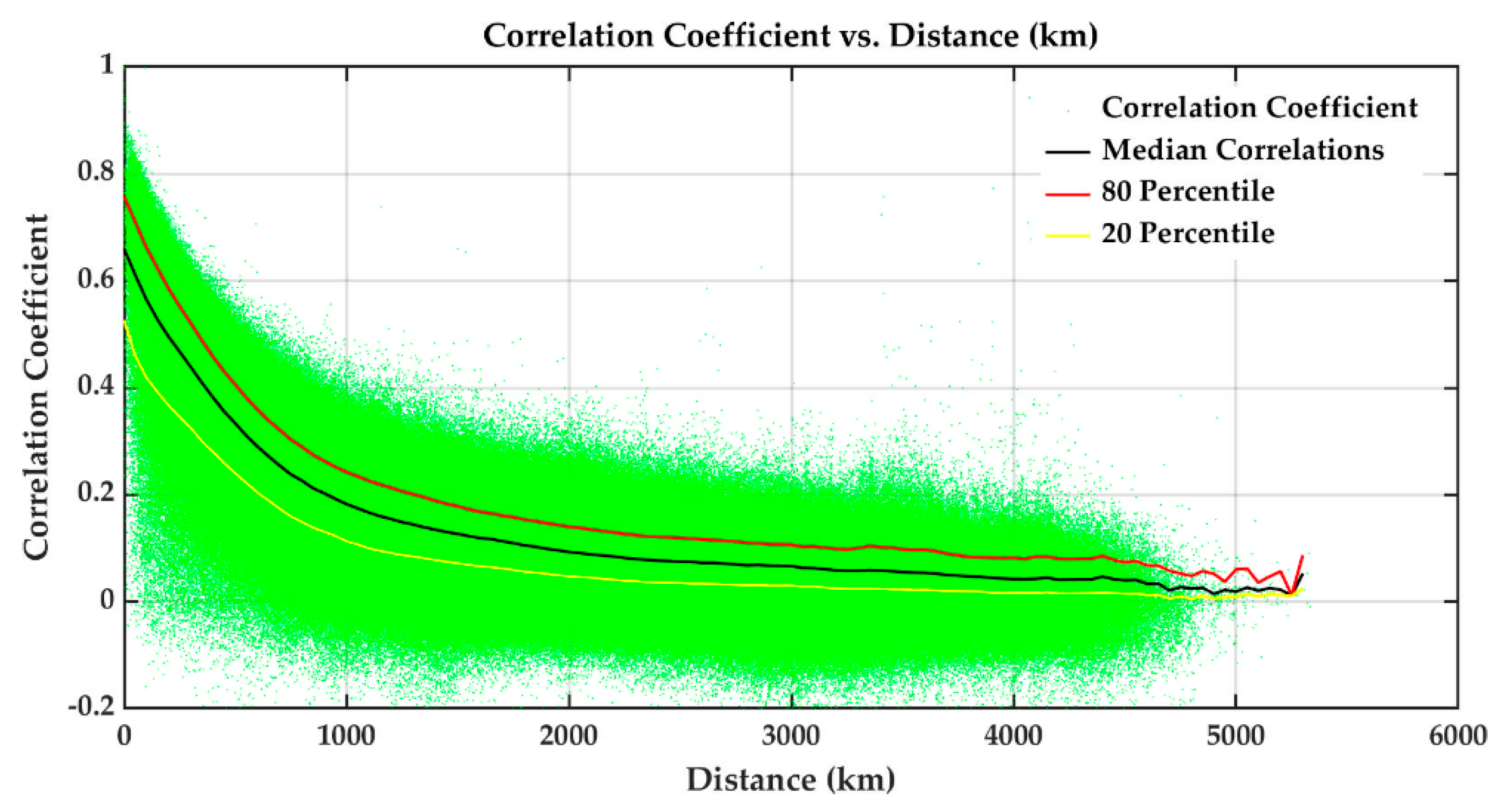
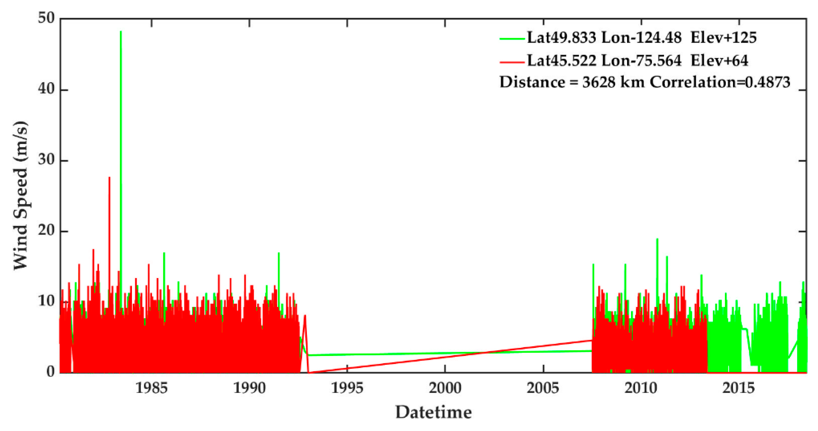
2.1. Correlation-Based Distance

In this study, the wind speed correlation is calculated for all the U.S. wind observation stations. The correlation coefficient is calculated for the WSTS according to Pearson correlation coefficient [50] (Equation (1)) as
ρ = i ( x i x ) ( y i y ) σ x σ y i ( x i x ) 2 i ( y i y ) 2     ,   ( 1 ρ 1 )
where x and y are sample variables of the WSTS vectors, x i   and   y i are individual sample points indexed with i. The wind speeds of two stations rise and fall synchronously in relative unison at ρ near one. A correlation coefficient near zero indicates that wind speeds vary independently of each other. A negative correlation coefficient would indicate anticorrelation between wind speeds. The Spherical law of cosines (Equation (2)) is used to calculate the distances between each pair of stations based on its longitude (lon) and latitude (lat) as
d = c o s 1 ( s i n φ 1 · s i n φ 2 + c o s φ 1 · c o s φ 2 · c o s Δ λ ) · R
where φ 1 is lat1, φ 2 is lat2, Δ λ = l o n 2 l o n 1 , and R is earth’s radius ≈ 6371 km.
For better illustration, eight stations of WSTS and locations in the four directions of the U.S. were extracted. They are located in California (CA), Texas (TX), South Dakota (SD), and New England (NE), see Figure 1. The common WSTS periods used in the spatial correlation calculations are shown in Figure 2. The correlation coefficient decreases slightly to 0.7 for the first 100 km distances as shown in Figure 3. By increasing the distance to 1400 km, the correlation decreases below 0.2. Past 2500 km the correlation coefficient is in the zero’s range. That depicts a general pattern of an inversely proportional relationship between the correlation value and the distance between stations that will be discussed in detail in the results section.

2.2. Map Optimization Fuzzy Logic Framework

Fuzzy logic is a form, which deals with reasoning and approximates in place of fixed and exact values. Unlike binary sets, it has real values in the range between 0 and 1, see [52]. An analytical technique with Fuzzy logic framework is used to evaluate U.S. map pixels and optimize new wind turbines locations. Different environmental, economic, and geographical parameters have been considered, represented in wind speed, terrain elevation, land use, and land price per acre.
The developed fuzzy logic model flowchart is shown in Figure 4. It has several phases included representing each factor as fuzzy sets, computing the spatial individual satisfaction degree, which quantifies the overall factor impact index and overlays the overall factors impact indices layers to define the site selections. The individual satisfaction degree of the function with respect to each factor is determined by using the membership functions of the fuzzy sets associated with the factor, see [53].
In the present work, map optimization has been applied for the lower 48 states of the U.S. The model has been calibrated by identifying the current wind turbines as unused fields with a land type correlated to the field coordinates at the land cover datasets. Our model results show that a percentage of 87.2% of the current sites are selected to be suitable for turbine placement.

3. Results and Discussion

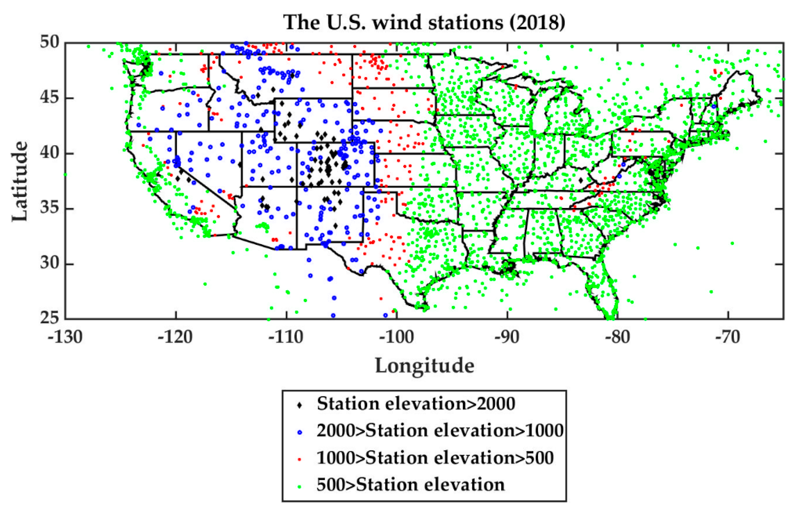
3.1. Database Development

The wind datasets in the following approach serve as inputs to realistic studies of characteristics, spatial correlations, capacity factors, WSTS analysis, and maps optimization. Beside the observational and predicted wind speed datasets, big geological, economic and urban datasets are used to perform new turbines placement optimization correlated to the current turbines to be integrated with the established electrical grid.

3.1.1. Observational Datasets

Observational horizontal wind data were gathered from the National Oceanic and Atmospheric Administration (NOAA), Climatic Data Center, Integrated Surface Database (ISD) [51,54]. The temporal distribution of the data covers wide periods ranging from 1960 to 2018. The data was preprocessed to unify the time scale. The different time scales were approximated to an hourly time scale. The spatial distribution of the ISD wind observational stations up to 2018 is shown in Figure 5, for the US stations and some neighbor stations from Canada and Mexico. In this, the elevation in meters (m) from the sea level to each station is classified into 4 ranges, where each of these ranges (higher than 2000 m, between 2000 m and 1000 m, between 1000 m and 500 m and less than 500 m) is marked with distinct colors.

3.1.2. Forecasted Datasets

The forecast wind speed time series is processed using the Wind Integration National Dataset (WIND) Toolkit [55,56,57,58]. The WIND Toolkit combines several instantaneous wind speeds forecast datasets from computer model output, from 2007 to 2013, over the contiguous U.S. The WIND database was generated on a 2 km by 2 km grid with a 20 m resolution from the ground to 160 m above ground. However, hourly WSTS data at a 100 m hub were considered in this work.

3.1.3. Map Optimization Datasets

The parameters of the elevations, land cover, and land price were used along with the wind speed for the map optimization process. Elevation dataset was collected from the 1/3rd arc-second (≈10 m resolution) Digital Elevation Models (DEMs) USGS National Map [59]. Each longitude and latitude tile was downloaded individually. Then, all tiles were merged together while the missing few tiles were interpolated. The land type and its use were collected from MODIS land cover type data product (MCD12Q1) [60], 5′ × 5′ resolution. The land prices were gathered for U.S. counties’ land price map [61]. Land price is divided within 9 categories based on the minimum and maximum land price per acre for each county. These categories are ranging from 1 $ to +73K $. The land price of each borderline separates between counties is proposed to be the same price of any of these mutual counties. The radial data sets, i.e., and land use were re-organized across Cartesian longitude and latitude as GIS layers. Resolutions were converted to a uniform grid resolution of (2 km × 2 km) to interrogate the overlay satisfaction for each grid node.

3.2. Correlation-Based Distance

Several studies used this approach to spatial-correlate the wind speed time series between limited wind farms within an individual region. In the underlying study, the spatial correlation between all available WSTSs for the observational wind stations (NOAA-ISD) was numerically calculated, while the wake effects from neighboring wind farms are neglected. Figure 6 displays the correlation between stations as a function of the distance between each pair of stations. The closest pair of stations are separated by 7 km and the farthest by 5400 km. The correlation value is inversely proportional to the distance since its value decreases rapidly with site separation. In this connection, it is worth mentioning that as far as we separated between sites, the probability of experiencing the same instantaneous wind speeds was decreasing.
According to the farm’s spatial interconnection necessity for electrical steady production, the correlation results show a satisfactory span of 100 km into large grids. Focusing on the Median, 80th, and 20th percentiles of the correlation-based distance, the curves are consistent with the correlation without overlapping for a distance up to 4500 km. The median line is centering the robust area, while it represents the local regression curve. An analytical form was fitted to calculate the correlation based on the mean correlation curve (Equation (3)).
r(x) = abx + cdx,
where x is the distance, and the fitting parameter are a = 0.574; b = −0.007889; c = 0.4024; d = −0.0006791.
It is of great importance to interpret the reasons for the presence of low correlation values for several cases related to stations with a short separation distance (less than 100 km), as well as those correlations with relatively high values for stations with a long separation distance (>3000 km). Different tools were used to explore the reasons such as Ad-hoc, and WSTS comparison, and territorial features analysis.
Ad-hoc analysis with color scatter plot of wind speed correlation for 313 stations uniformly distributed over the U.S. stations is illustrated in Figure 7. The colors indicate the average period of the WSTS used in the correlation calculation. The graph shows a more coherent correlation curve for the recent WSTS correlations periods in the current century (2000 y or after). The WSTS periods before 2000 showing many relatively highly correlated stations of long distances are discussed in the next paragraph.
The mutual WSTSs used in the calculation were inspected for several pairs of wind observation stations to identify if the reason for such an odd correlation value is due to measurement uncertainties. The inspection showed that measurement uncertainties are a reason for a few low correlation values for stations spaced with a short distance and/or high correlation at a long distance. An example of such errors in measurement reports is shown in Figure 8, where zero wind speed values are noted for a station during the entire period from 2014 to 2018.
The terrain features were investigated for other closed sites that have odd correlation values. It was found that, in many cases the terrain features cause irregular correlation values mainly because of the elevation height difference between those stations is significant. Figure 9 shows an example of such cases for a site pair located at (33.933 N 118.4 W; 34.750 N 118.73 W). The distance between sites is 96 km, but the elevation height difference is 1300 m [62], which interpret the WSTS correlation value 0.4. Hence, we can conclude that measurement uncertainties and terrain feature topography are the main reasons for the presence of low/high correlation irregular values at short/long distances, respectively. It is also important to mention that the terrain features affect the wind turbine installation, operational safety, construction sequence, and performance [63].

3.3. Available and Ideal Power Capacity

Wind turbines convert the available power nested in wind speed to electricity. The power generation of a wind turbine is a function of the wind speed and the wind turbine characteristics. The relation between a wind turbine power generation and the wind speed variation is represented in a power curve [64]. Power generation from a turbine requires that wind speeds fall in a specific range, i.e., between cut-in and cut-off speeds. Wind speed must be higher than the cut-in speed to start power generating, while a zero power output is present below this value. Also, the wind turbine stops generating power at speeds greater than the cut-off speed, to prevent damage. Therefore, wind turbine power production increases with increasing wind speed between the cut-in and the cut-off speeds range till a rated value in which the maximum power generation of the turbine is reached and attained till the cut-off speed.
The number of wind turbines in the U.S. until July 2020 exceeded 64,553 with a total rated capacity of 94,105 MW [27]. In this regard, we try in this contribution to answer the question related to the maximum power capacity available for generation in the ideal case (100% utilization of wind sources). The WIND dataset used to estimate the total mean power capacity is related to the current wind fields in the U.S. It is calculated by extracting the WSTS for each wind site by matching its location (longitude and latitude) with the closest grid point in WIND database. This is followed by summing all the time series into a single time series by considering the wind farm capacity as the weight of the sum. WSTS for each field is multiplied with the number of turbines and its capacities. The mean-time series show that the total power capacity available in the ideal case is equal to 154,350 MW, which is significant in comparison to 94,105 MW of the actual production. In other words, this indicates that U.S. wind turbines are currently utilizing approximately 61% of the total wind resources available in the current wind turbines sites.

3.4. Wind Seasonality

A state of seasonality trends for the magnitude and variability of wind speed was observed in the WSTS in both observational and predicted datasets. Periodicity is a crucial factor since it gives the ability to do preliminary forecasting of wind resources available for each season and thereby the power capacities. WSTS analysis helps in controlling the seasonal power generation integrated into the grid. It is essential to design the required strategies to meet the power demand extremes for each season and handle the peak times situations. However, the diversity of the time series dataset, based on location, elevation, and atmospheric circulation, is directed to deal with the mean WSTS for all U.S. stations to reveal the general wind tendency for each season. The mean WSTS (WIND dataset) for 7 years is illustrated in Figure 10, where the WSTS evolution exhibits a periodic pattern reflecting wind seasonality. The mean wind speed falls in a range from 7 to 12 m/s.
To educe the periodicity for the fluctuated WSTS, an analytical function is fitted using MATLAB curve fitting toolbox [65]. By applying a variety of post-processing fitting methods, a sine wave annual periodic curve is detected. In particular, it is explained in Equation (4) with a 95% coefficients confidence bounds.
y = a1 sin (b1x + c1) + a2 sin (b2x + c2) + a3 sin (b3x + c3),
where a1 = 95.93; b1 = 4.257 × 10⁻⁵; c1 = 0.2598; a2 = 86.39; b2 = 4.508 × 10⁻⁵; c2 = 3.325; a3 = 1.954; b3 = 0.0007167; c3 = −0.8267; x = 1:61,368. The corresponding power spectrum in Figure 11 shows a more uniform distribution of energy among a wide range of frequencies. The power spectrum peaks present non-dimensional main, secondary, and harmonic frequencies that correspond to dimensional yearly, semiyearly, and daily periods, respectively. During each yearly cycle, mean wind speed exhibits a medium wind speed range twice in spring and autumn, while it exhibits maximum and minimum ranges once a year in summer and winter, respectively. Therefore, the power generation from wind energy is maximized during the summer and minimized during winter. The harmonic peak shows the daily repetition of the wind speed, which gradually increases from midnight to noon then decreases from noon to midnight.

3.5. Map Optimization

The fuzzy logic approach is applied for the optimization of new wind turbines placement. The approach identifies the suitable locations for wind turbines based on different criteria of suitability by which an area is then being rated. The considered layers are wind speed, land use, land price, and terrain elevations. These parameters represent different aspects including physical resources, economic costs, terrain features, and urban occupancy. A uniform spatial mesh grid for the contiguous U.S. is used in this work with a resolution of 2 km by 2 km.
First, a wind speed mask is applied to classify the locations rich with wind sources. A minimum mean-wind-speed of 6 m/s is considered for a potential wind farm site, according to previous studies [35,66,67]. Then, the land cover layer classifies the land type and occupancy of each location. In terms of land cover, the highest satisfaction degree is given to the croplands, grasslands, and vegetation areas [37]. The elevation and land price layers identify the installation complexity and relative costs. In the final stage, the individual satisfaction associated with each location is interrogated into a single value according to its overall satisfaction for all considered parameters.
Figure 12, shows suitable locations for new installations of the wind turbines. Most of the sites are located in the Midwest, Oklahoma, and Texas. Also, it must be noted that the West Coast and Middle Atlantic regions show several suitable locations. The results show that 63% of the suitable sites for turbine placements are in agreement with an overall performance index of 0.5. It is obvious that the variances in the elevation and the land prices affect strongly the overall satisfaction. Several locations rich in wind resources are technically rejected because of the land price, especially on the East Coast. Similarly, various locations are not selected in relatively large-scale regions because of their elevations, such as in the Mountain West region.
The priority sites, illustrated in Figure 13, are considered so that an overall satisfaction performance index of 0.7 is fulfilled. Moreover, a minimum setback distance, between the proposed location and the closest residential border, of 2 km is integrated into the model for safety purposes. Those sites are considered as optimum locations. The distances between the current and targeted turbine locations are also investigated. It is found that 87% of each targeted site is located close to current wind turbine farms with a distance ≤ 50 km. This distance value is in good agreement with the recommendations extracted from the correlation-based distance approach. Furthermore, it is necessary to observe that this relatively short distance confirms that the optimum sites will potentially assist the current electricity grid by increasing a steady power generation. Therefore, the U.S. Bureau of Land Management (BLM) provides a high priority processing when the proposed wind turbine location is relatively adjacent to the previously disturbed or developed sites [47].

4. Conclusions

In the present work, observational and predicted wind energy datasets were analyzed. Correlation, power capacity and wind seasonality approaches were implemented using the entire datasets to analyze different aspects. Also, we proposed and validated a numerical approach based on a novel fuzzy logic framework for optimizing suitable sites for new wind turbine placements. A correlation-based distance approach of the observational WSTS for all the U.S. stations has shown an inversely proportional relation between correlation and distance. Good correlation values were noted for stations separated with a short span of ≤100 km. Therefore, installing new turbines close to the current ones would assist the current electrical grids. The analysis has shown that the computed uncertainties and the terrain features affect the correlation values.
The total power capacity available for optimum utilization of the wind resources indicates that the current wind turbines are utilizing approximately 61% of the wind resources available in the turbine’s sites. The evolution of wind speed with time was also analyzed. The generated WSTS represented a periodic sine wave pattern, thus, reflecting the wind seasonality. The power spectrum indicated that main, secondary, and harmonic frequencies correspond to wind speed periodic pattern yearly, semiyearly, and daily. Yearly, the mean wind speed exhibits a medium-range twice in spring and autumn, while it exhibits maximum and minimum wind speed ranges once a year in summer and winter, respectively. Daily, the wind speed gradually increases from midnight to noon then decreases from noon to midnight.
Map optimization approach using a fuzzy logic model was proposed for the optimization of wind turbine placement. The model was adopted by integrating different parameters presented in wind speed, land use, price, and elevation. Suitable and priority sites were classified based on overall satisfaction values. The targeted sites are in general agreement with the recommendation of the correlation approach. The wind turbine site selection topic is broad and proposes that the future research direction will include deep learning approaches.

Author Contributions

G.A. did the research, finalized the results at Columbia University, and wrote the paper with some guidance from M.A.-N. and A.E.A. All authors have read and agreed to the published version of the manuscript.

Funding

M. Al-Numay and A. El Aroudi acknowledge financial support from the Researchers Supporting Project number (RSP-2021/150), King Saud University, Riyadh, Saudi Arabia.

Institutional Review Board Statement

Not applicable.

Informed Consent Statement

Not applicable.

Data Availability Statement

The datasets used in this work are available online through their original sources as follows: Observational wind speed datasets from the National Oceanic and Atmospheric Administration (NOAA) Climatic Data Center, Integrated Surface Database (ISD). Available: https://www.ncdc.noaa.gov/isd (accessed on 30 August 2018). The predicted hourly wind speed time series dataset at a 100-m hub is available on Wind Integration National Dataset (WIND) Toolkit. Available: https://www.nrel.gov/grid/wind-toolkit.html (accessed on 30 August 2018). The land elevation dataset is available on 1/3rd arc-second Digital Elevation Models (USGS National Map). Available: https://catalog.data.gov/dataset/national-elevation-dataset-ned-1-3-arc-second-downloadable-data-collection-national-geospatial (accessed on 30 August 2018). The land type and its use are available on MODIS land cover type data product (MCD12Q1), 5′ × 5′ resolution. Available: https://lpdaac.usgs.gov/products/mcd12q1v006/ (accessed on 30 August 2018) The U.S. counties land price map. Available: https://decolonialatlas.files.wordpress.com/2017/12/us-counties-land-price-per-acre-map.jpg (accessed on 30 August 2018).

Acknowledgments

We acknowledge the National Aeronautics and Space Administration (NASA), National Oceanic and Atmospheric Administration (NOAA), United States Geological Survey (USGS), The Global Land Cover Facility (GLCF), Land Processes Distributed Active Archive Center (LP-DAAC), American Wind Energy Association (AWEA) and Lawrence Berkeley National Laboratory (LBNL) for supporting the required big datasets used in this work. Also, G.A. acknowledges supervision from Marco Giometto, Mostafa Momen and support from the department of Civil Engineering and Engineering Mechanics at Columbia University during his research stay. M. Al-Numay and A. El Aroudi acknowledge financial support from the Researchers Supporting Project number (RSP-2021/150), King Saud University, Riyadh, Saudi Arabia.

Conflicts of Interest

The author declares no conflict of interest regarding the publication of this paper.

References

  1. Schaeffer, R.; Szklo, A.S.; de Lucena, A.F.P.; Borba, B.S.M.C.; Nogueira, L.P.P.; Fleming, F.P.; Troccoli, A.; Harrison, M.; Boulahya, M.S. Energy sector vulnerability to climate change: A review. Energy 2012, 38, 1–12. [Google Scholar] [CrossRef]
  2. Prema, V.; Rao, K.U. Time series decomposition model for accurate wind speed forecast. Renew. Wind Water Sol. 2015, 2, 18. [Google Scholar] [CrossRef] [Green Version]
  3. Gadalla, M.A.; Olujic, Z.; Jansens, P.J.; Jobson, M.; Smith, R. Reducing CO2 emissions and energy consumption of heat-integrated distillation systems. Environ. Sci. Technol. 2005, 39, 6860–6870. [Google Scholar] [CrossRef]
  4. Tourn, S.; Pallarès, J.; Cuesta, I.; Paulsen, U.S. Characterization of a new open jet wind tunnel to optimize and test vertical axis wind turbines. J. Renew. Sustain. Energy 2017, 9, 033302. [Google Scholar] [CrossRef] [Green Version]
  5. Abdelaziz, O.Y.; Hosny, W.M.; Gadalla, M.A.; Ashour, F.H.; Ashour, I.A.; Hulteberg, C.P. Novel process technologies for conversion of carbon dioxide from industrial flue gas streams into methanol. J. CO2 Util. 2017, 21, 52–63. [Google Scholar] [CrossRef]
  6. Pryor, S.C.; Barthelmie, R.J.; Young, D.T.; Takle, E.S.; Arritt, R.W.; Flory, D.; Gutowski, W.J.; Nunes, A.; Roads, J. Wind speed trends over the contiguous United States. J. Geophys. Res. 2009, 114, D14105. [Google Scholar] [CrossRef]
  7. Holt, E.; Wang, J. Trends in wind speed at wind turbine height of 80 m over the contiguous United States using the north American Regional Reanalysis (NARR). J. Appl. Meteorol. Climatol. 2012, 51, 2188–2202. [Google Scholar] [CrossRef] [Green Version]
  8. Hertwich, E.G.; Gibon, T.; Bouman, E.A.; Arvesen, A.; Suh, S.; Heath, G.A.; Bergesen, J.D.; Ramirez, A.; Vega, M.I.; Shi, L. Integrated life-cycle assessment of electricity-supply scenarios confirms global environmental benefit of low-carbon technologies. Proc. Natl. Acad. Sci. USA 2015, 112, 6277–6282. [Google Scholar] [CrossRef] [Green Version]
  9. Sanchez, V.; Pallares, J.; Vernet, A.; Agafonova, O.; Hämäläinen, J. A Multiple Actuator Block model for vertical axis wind turbines. Renew. Energy 2016, 99, 592–601. [Google Scholar] [CrossRef]
  10. Pryor, S.C.; Barthelmie, R.J. Assessing climate change impacts on the near-term stability of the wind energy resource over the United States. Proc. Natl. Acad. Sci. USA 2011, 108, 8167–8171. [Google Scholar] [CrossRef] [PubMed] [Green Version]
  11. Albadi, M.H.; El-Saadany, E.F. Overview of wind power intermittency impacts on power systems. Electr. Power Syst. Res. 2010, 80, 627–632. [Google Scholar] [CrossRef]
  12. Velandia-Cardenas, C.; Vidal, Y.; Pozo, F. Wind Turbine Fault Detection Using Highly Imbalanced Real SCADA Data. Energies 2021, 14, 1728. [Google Scholar] [CrossRef]
  13. Florescu, A.; Barabas, S.; Dobrescu, T. Research on Increasing the Performance of Wind Power Plants for Sustainable Development. Sustainability 2019, 11, 1266. [Google Scholar] [CrossRef] [Green Version]
  14. Tang, M.; Zhao, Q.; Ding, S.X.; Wu, H.; Li, L.; Long, W.; Huang, B. An Improved LightGBM Algorithm for Online Fault Detection of Wind Turbine Gearboxes. Energies 2020, 13, 807. [Google Scholar] [CrossRef] [Green Version]
  15. Ma, H.; Oxley, L.; Gibson, J.; Li, W. A survey of China’s renewable energy economy. Renew. Sustain. Energy Rev. 2010, 14, 438–445. [Google Scholar] [CrossRef]
  16. Pryor, S.C.; Barthelmie, R.J.; Clausen, N.E.; Drews, M.; MacKellar, N.; Kjellström, E. Analyses of possible changes in intense and extreme wind speeds over northern Europe under climate change scenarios. Clim. Dyn. 2012, 38, 189–208. [Google Scholar] [CrossRef]
  17. Türksoy, F. Investigation of wind power potential at Bozcaada, Turkey. Renew. Energy 1995, 6, 917–923. [Google Scholar] [CrossRef]
  18. Barthelmie, R.J.; Courtney, M.S.; Højstrup, J.; Larsen, S.E. Meteorological aspects of offshore wind energy: Observations from the Vindeby wind farm. J. Wind Eng. Ind. Aerodyn. 1996, 62, 191–211. [Google Scholar] [CrossRef]
  19. Xiao, Y.Q.; Li, Q.S.; Li, Z.N.; Chow, Y.W.; Li, G.Q. Probability distributions of extreme wind speed and its occurrence interval. Eng. Struct. 2006, 28, 1173–1181. [Google Scholar] [CrossRef]
  20. National Renewable Energy Laboratory. 20% Wind Energy by 2030: Increasing Wind Energy’s Contribution to US Electricity Supply; US Department of Energy: Washington, DC, USA, 2008; pp. 399–404.
  21. Kempton, W.; Pimenta, F.M.; Veron, D.E.; Colle, B.A. Electric power from offshore wind via synoptic-scale interconnection. Proc. Natl. Acad. Sci. USA 2010, 107, 7240–7245. [Google Scholar] [CrossRef] [Green Version]
  22. St. Martin, C.M.; Lundquist, J.K.; Handschy, M.A. Variability of interconnected wind plants: Correlation length and its dependence on variability time scale. Environ. Res. Lett. 2015, 10. [Google Scholar] [CrossRef]
  23. Katzenstein, W.; Fertig, E.; Apt, J. The variability of interconnected wind plants. Energy Policy 2010, 38, 4400–4410. [Google Scholar] [CrossRef]
  24. Kahn, E. The reliability of distributed wind generators. Electr. Power Syst. Res. 1979, 2, 1–14. [Google Scholar] [CrossRef]
  25. Oswald, J.; Raine, M.; Ashraf-Ball, H. Will British weather provide reliable electricity? Energy Policy 2008, 36, 3212–3225. [Google Scholar] [CrossRef]
  26. Sinden, G. Characteristics of the UK wind resource: Long-term patterns and relationship to electricity demand. Energy Policy 2007, 35, 112–127. [Google Scholar] [CrossRef]
  27. Hoen, B.D.; Diffendorfer, J.E.; Rand, J.T.; Kramer, L.A.; Garrity, C.P.; Hunt, H.E. United States Wind Turbine Database (ver. 3.1, July 2020): U.S. Geological Survey, American Wind Energy Association, and Lawrence Berkeley National Laboratory Data Release. 2020. Available online: https://www.sciencebase.gov/catalog/item/57bdfd8fe4b03fd6b7df5ff9 (accessed on 21 September 2021).
  28. Zergane, S.; Smaili, A.; Masson, C. Optimization of wind turbine placement in a wind farm using a new pseudo-random number generation method. Renew. Energy 2018, 125, 166–171. [Google Scholar] [CrossRef]
  29. Naderipour, A.; Abdul-Malek, Z.; Nowdeh, S.A.; Gandoman, F.H.; Moghaddam, M.J.H. A multi-objective optimization problem for optimal site selection of wind turbines for reduce losses and improve voltage profile of distribution grids. Energies 2019, 12, 2621. [Google Scholar] [CrossRef] [Green Version]
  30. Marmidis, G.; Lazarou, S.; Pyrgioti, E. Optimal placement of wind turbines in a wind park using Monte Carlo simulation. Renew. Energy 2008, 33, 1455–1460. [Google Scholar] [CrossRef]
  31. Noorollahi, Y.; Yousefi, H.; Mohammadi, M. Multi-criteria decision support system for wind farm site selection using GIS. Sustain. Energy Technol. Assess. 2016, 13, 38–50. [Google Scholar] [CrossRef]
  32. Cassola, F.; Burlando, M.; Antonelli, M.; Ratto, C.F. Optimization of the Regional Spatial Distribution of Wind Power Plants to Minimize the Variability of Wind Energy Input into Power Supply Systems. J. Appl. Meteorol. Climatol. 2008, 47, 3099–3116. [Google Scholar] [CrossRef]
  33. Ituarte-Villarreal, C.M.; Espiritu, J.F. Optimization of wind turbine placement using a viral based optimization algorithm. Procedia Comput. Sci. 2011, 6, 469–474. [Google Scholar] [CrossRef] [Green Version]
  34. Malvaldi, A.; Weiss, S.; Infield, D.; Browell, J.; Leahy, P.; Foley, A.M. A spatial and temporal correlation analysis of aggregate wind power in an ideally interconnected Europe. Wind Energy 2017, 20, 1315–1329. [Google Scholar] [CrossRef] [Green Version]
  35. Cetinay, H.; Kuipers, F.A.; Guven, A.N. Optimal siting and sizing of wind farms. Renew. Energy 2017, 101, 51–58. [Google Scholar] [CrossRef] [Green Version]
  36. Van Haaren, R.; Fthenakis, V. GIS-based wind farm site selection using spatial multi-criteria analysis (SMCA): Evaluating the case for New York State. Renew. Sustain. Energy Rev. 2011, 15, 3332–3340. [Google Scholar] [CrossRef]
  37. Denholm, P.; Hand, M.; Jackson, M.; Ong, S. Land Use Requirements of Modern Wind Power Plants in the United States; National Renewable Energy Lab.: Golden, CO, USA, 2009. [Google Scholar] [CrossRef] [Green Version]
  38. Knopper, L.D.; Ollson, C.A.; McCallum, L.C.; Aslund, M.L.W.; Berger, R.G.; Souweine, K.; McDaniel, M. Wind turbines and human health. Front. Public Health 2014, 2, 1–30. [Google Scholar] [CrossRef] [Green Version]
  39. Saidur, R.; Rahim, N.A.; Islam, M.R.; Solangi, K.H. Environmental impact of wind energy. Renew. Sustain. Energy Rev. 2011, 15, 2423–2430. [Google Scholar] [CrossRef]
  40. Kwong, W.Y.; Zhang, P.Y.; Romero, D.; Moran, J.; Morgenroth, M.; Amon, C. Wind Farm Layout Optimization Considering Energy Generation and Noise Propagation. In Volume 3: 38th Design Automation Conference, Parts A and B; ASME: Chicago, IL, USA, 12–15 August 2012; p. 323. [Google Scholar]
  41. Katinas, V.; Marčiukaitis, M.; Tamašauskienė, M. Analysis of the wind turbine noise emissions and impact on the environment. Renew. Sustain. Energy Rev. 2016, 58, 825–831. [Google Scholar] [CrossRef]
  42. Yin Kwong, W.; Yun Zhang, P.; Romero, D.; Moran, J.; Morgenroth, M.; Amon, C. Multi-Objective Wind Farm Layout Optimization Considering Energy Generation and Noise Propagation With NSGA-II. J. Mech. Des. 2014, 136, 091010. [Google Scholar] [CrossRef]
  43. Stemler, J. Wind Power Siting, Incentives, and Wildlife Guidelines in the United States. 2007. Available online: https://www.fws.gov/habitatconservation/windpower/afwa%20wind%20power%20final%20report.pdf (accessed on 21 September 2021).
  44. Heibel, J.; Durkay, J. State Statutes on Wind Facility Siting. State Legislative Approaches to Wind Energy Facility Siting. 2016. Available online: https://www.ncsl.org/research/energy/state-wind-energy-siting.aspx#statutes.v (accessed on 21 September 2021).
  45. Shepherd, D.; Welch, D.; Hill, E.; McBride, D.; Dirks, K. Evaluating the impact of wind turbine noise on health-related quality of life. Noise Health 2011, 13, 333. [Google Scholar] [CrossRef]
  46. Davy, J.L.; Burgemeister, K.; Hillman, D. Wind turbine sound limits: Current status and recommendations based on mitigating noise annoyance. Appl. Acoust. 2018, 140, 288–295. [Google Scholar] [CrossRef]
  47. Land Management Bureau-U.S. Department of the Interior Competitive Processes, Terms, and Conditions for Leasing Public Lands for Solar and Wind Energy Development and Technical Changes and Corrections. Fed. Regist. 2016, 81 FR 9212, 92122–92230. [Google Scholar]
  48. Land Management Bureau-U.S. Department of the Interior Rights-of-way under the Federal Land Policy Management Act. 2018. Available online: https://www.blm.gov/sites/blm.gov/files/AboutUs_LawsandRegs_FLPMA.pdf (accessed on 21 September 2021).
  49. Dhunny, A.Z.; Doorga, J.R.S.; Allam, Z.; Lollchund, M.R.; Boojhawon, R. Identification of optimal wind, solar and hybrid wind-solar farming sites using fuzzy logic modelling. Energy 2019, 188, 116056. [Google Scholar] [CrossRef]
  50. Pearson, K. Notes on the History of Correlation. Biometrika 1920, 13, 25. [Google Scholar] [CrossRef]
  51. NOAA National Centers for Environmental Information: Global Surface Hourly, Integrated Surface Dataset. 2017. Available online: https://data.noaa.gov/dataset/dataset/integrated-surface-dataset-global (accessed on 21 September 2021).
  52. Novák, V.; Perfilieva, I.; Močkoř, J. Mathematical Principles of Fuzzy Logic; Springer: Boston, MA, USA, 1999; ISBN 978-1-4613-7377-3. [Google Scholar]
  53. Ling, W.-K. REVIEWS. In Nonlinear Digital Filters; Elsevier: Amsterdam, The Netherlands, 2007; pp. 8–31. [Google Scholar]
  54. Smith, A.; Lott, N.; Vose, R. The Integrated Surface Database: Recent Developments and Partnerships. NOAA’s National Climatic Data Center. Bull. Am. Meteorol. Soc. 2011, 92, 704–708. [Google Scholar] [CrossRef]
  55. Draxl, C.; Clifton, A.; Hodge, B.-M.; McCaa, J. The Wind Integration National Dataset (WIND) Toolkit. Appl. Energy 2015, 151, 355–366. [Google Scholar] [CrossRef] [Green Version]
  56. King, J.; Clifton, A.; Hodge, B.; King, J. Validation of Power Output for the WIND Toolkit; National Renewable Energy Lab.: Golden, CO, USA, 2014. [Google Scholar]
  57. Draxl, C.; Hodge, B.; Clifton, A. Overview and Meteorological Validation of the Wind Integration National Dataset Toolkit. National Renewable Energy Lab. 2015. Available online: https://www.nrel.gov/docs/fy15osti/61740.pdf (accessed on 21 September 2021).
  58. Draxl, C.; Clifton, A. A Guide to Using the WIND Toolkit Validation Code. National Renewable Energy Lab. 2014. Available online: https://www.nrel.gov/docs/fy15osti/62595.pdf (accessed on 21 September 2021).
  59. U.S. Geological Survey. 1/3rd arc-second Digital Elevation Models (DEMs)-USGS National Map 3DEP Downloadable Data Collection: U.S. Geological Survey. 2017. Available online: https://www.sciencebase.gov/catalog/item/4f70aa9fe4b058caae3f8de5 (accessed on 21 September 2021).
  60. Friedl, M.A.; Sulla-Menashe, D.; Tan, B.; Schneider, A.; Ramankutty, N.; Sibley, A.; Huang, X. MODIS Collection 5 global land cover: Algorithm refinements and characterization of new datasets. Remote Sens. Environ. 2010, 114, 168–182. [Google Scholar] [CrossRef]
  61. US Counties Land Price per Acre Map. Available online: https://decolonialatlas.files.wordpress.com/2017/12/us-counties-land-price-per-acre-map.jpg (accessed on 21 September 2021).
  62. Google. (n.d.-b). Wind Stations Locations. Retrieved from Google Maps. 2020. Available online: https://www.google.com/maps/@34.2297666,-118.6235017,125623m/data=!3m1!1e3 (accessed on 21 September 2021).
  63. Sedlacek, G.; Miehe, A.; Libreros, A.; Heider, Y. Geotechnical Stability of Gravity Base Foundations for Offshore Wind Turbines on Granular Soils. In Proceedings of the ASME 2012 31st international conference on ocean, offshore and Arctic engineering, American Society of Mechanical Engineers, Rio de Janeiro, Brazil, 1–6 July 2012; pp. 57–63. [Google Scholar]
  64. Dhople, S.V.; Dominguez-Garcia, A.D. A framework to determine the probability density function for the output power of wind farms. In Proceedings of the 2012 IEEE North American Power Symposium (NAPS), Champaign, IL, USA, 9–11 September 2012; pp. 1–6. [Google Scholar]
  65. Curve Fitting Toolbox: For Use with MATLAB®; User’s Guide: Natick, MA, USA, 2017.
  66. Lynch, K.; Murphy, J.; Serri, L.; Airoldi, D. Site Selection Methodology for Combined Wind and Ocean Energy Technologies In Europe. In Proceedings of the 4th International Conference of Ocean Energy, Dublin, Ireland, 17–19 October 2012. [Google Scholar]
  67. Cradden, L.; Kalogeri, C.; Barrios, I.M.; Galanis, G.; Ingram, D.; Kallos, G. Multi-criteria site selection for offshore renewable energy platforms. Renew. Energy 2016, 87, 791–806. [Google Scholar] [CrossRef] [Green Version]
Figure 1. Locations of the selected stations in California, Texas, South Dakota, and New England. Data are from [51].
Energies 14 06127 g001
Figure 2. Common WSTS periods used in the calculation of the spatial correlation coefficient for the selected stations in CA, TX, SD, and NE.
Energies 14 06127 g002
Figure 3. Pair correlation for 8 selected stations in California, Texas, South Dakota, and New England.
Energies 14 06127 g003
Figure 4. Flowchart of the developed Fuzzy logic framework site selection model.
Energies 14 06127 g004
Figure 5. The spatial distribution of the integrated stations of ISD dataset up to 2018. The colors indicate the elevation in meters (m) from the sea level. The black dots indicate sites with elevations higher than 2000 m; blue dots for elevations from 1000 to 2000 m; red small dots for elevations from 500 to 1000 m; and green small dots for elevations less than 500 m. Data are from [51].
Energies 14 06127 g005
Figure 6. Correlation-based distance (km), for all U.S. wind stations. The green dots represent the correlation values. The black curve is the median; the yellow curve is the 20 percentiles; the red curve is the 80 percentiles.
Energies 14 06127 g006
Figure 7. Correlation-based distance (in km) for 313 wind stations distributed over the U.S. lower 48 states. The sample color indicates the time series period. Blue dots for later than 2012; green cycles for 2006 to 2012; red cycles for 2000 to 2006; and triangles before 2000. The black curve is the median; the yellow curve is the 20 percentiles; the red curve is the 80 percentiles.
Energies 14 06127 g007
Figure 8. WSTS tracking for two stations with relatively high correlations at distancing = 3628 km.
Energies 14 06127 g008
Figure 9. Territorial features comparison for spots with negative correlations while distancing = 96 km [62].
Energies 14 06127 g009
Figure 10. The mean wind speed time series.
Energies 14 06127 g010
Figure 11. Power spectrum for the wind speed.
Energies 14 06127 g011
Figure 12. Suitable sites for new wind turbine placement.
Energies 14 06127 g012
Figure 13. Priority selected sites for new wind turbine placement.
Energies 14 06127 g013
Publisher’s Note: MDPI stays neutral with regard to jurisdictional claims in published maps and institutional affiliations.

