Relay Identification Using Shifting Method for PID Controller Tuning

Abstract

The aim of this study was to present a relay shifting method for relay feedback identification of dynamical systems suitable for PID controller tuning. The proposed technique uses a biased relay to determine frequency response points from a single experiment without any assumptions about a model transfer function. The method is applicable for open-loop stable, unstable, and integration processes, even with a delay, and regardless of whether they are oscillating or non-oscillating. The core of this technique was formed by the so-called relay shifting filter. In this study, the method was applied to a parameter estimation of a second-order time-delayed (SOTD) model that can describe, with acceptable accuracy, the dynamics of most processes (even with a transport delay) near the operating point. Simultaneously, a parameter setting for the PID controller was derived based on the model parameters. The applicability of the proposed method was demonstrated on various simulated processes and tested on real laboratory apparatuses.

1. Introduction

In the process industry, relay feedback identification is popularly used for estimating model parameters. The relay control was originally used for process identification by Rotač [1]. This approach has been increasingly explored in recent years due to the relay feedback method suggested by Åström and Hägglund [2] for PID controller tuning. In the relay feedback test, the period of oscillation and the amplitude of the process output were measured. The critical gain and the critical frequency were determined by the describing function. For more details about the describing function, see [3]. The same parameters can also be estimated using the continuous cycling method by Ziegler and Nichols [4]. However, with the relay feedback method proposed by Åström and Hägglund, one can obtain these parameters without a priori information about the process in a controlled manner and in a shorter time. The critical frequency and the critical gain can be utilized for the estimation of one point on the process frequency response. However, the knowledge of one frequency point only allows for the estimation of two model parameters. Therefore, models with a relatively small number of parameters are predominantly used for modeling. Most often, these are first- or second-order time-delayed linear models. To obtain the model parameters of these simple models from the relay feedback test, Luyben [5] assumed that the steady-state gain was already known and estimated the dead time from the initial response. Shen et al. [6] suggested using a biased relay for the steady-state gain estimation. Li et al. [7] proposed using two relay feedback tests, wherein the second test runs with an additional transport delay. Be et al. showed that multiple frequency response points can be estimated from a single relay feedback test using a parasitic relay and the FFT algorithm [8]. In [9], Chidambaram and Sathe describe another possibility, in which the exponential attenuation factor of the expression is used in the Laplace transform. At present, more publications exist that are devoted to relay-based parametric estimation techniques for control purposes. A summary of the obtained results can be found in survey publications, for example, [9,10,11,12,13,14].

The existing relay identification methods often assume that the processes are at a steady state, use several relay feedback tests, do not consider disturbances, and pre-suppose knowledge about the transport delay or the static gain. Most methods are further associated with the type of process (underdamped/overdamped, stable/integrating/unstable). In the work by Sánchéz et al. [15], it is shown that there are only two methods for measuring several frequency response points in only one relay experiment. The first one is based on the Laplace transform of input and output, for example, [9,16], and the second method is the shifting method described in [17,18]. The extension of the basic shifting method and its use for overdamped systems is described in [15].

The aim of this paper is to present the relay shifting method for identifying various types of dynamical systems and for tuning PID controllers. First, the relay shifting method was derived, which helps to determine multiple frequency response points from a single experiment without any assumptions about the model transfer function. Then the proposed method was applied to fit the SOTD model to a wide range of processes with various properties (underdamped/overdamped, stable/integrating/unstable, and time-delayed systems). A derivation of PID controller parameters for the control of the stable process described by the SOTD model is given in Section 6. Section 5 and Section 7 describe the experimental results. Finally, the essential properties of the shifting method are summarized.

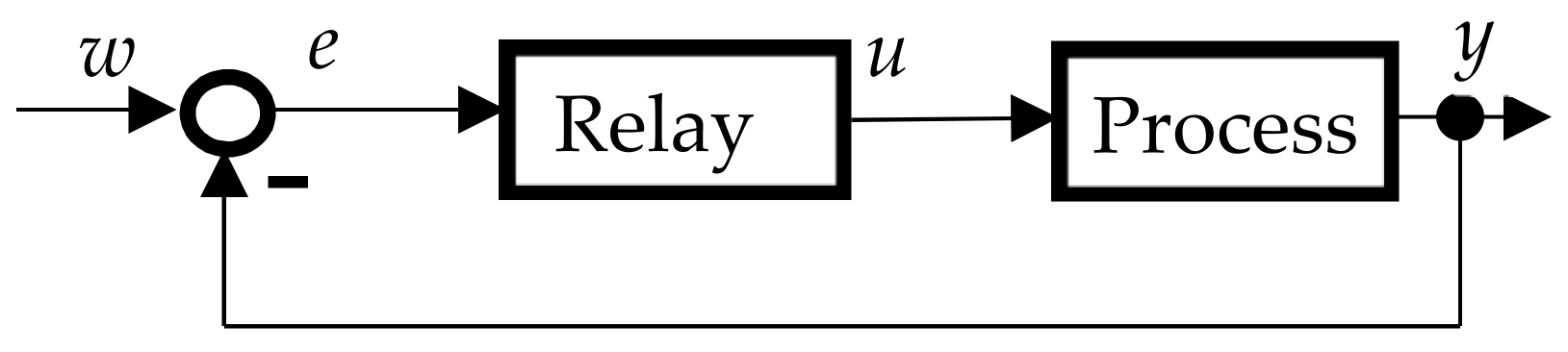
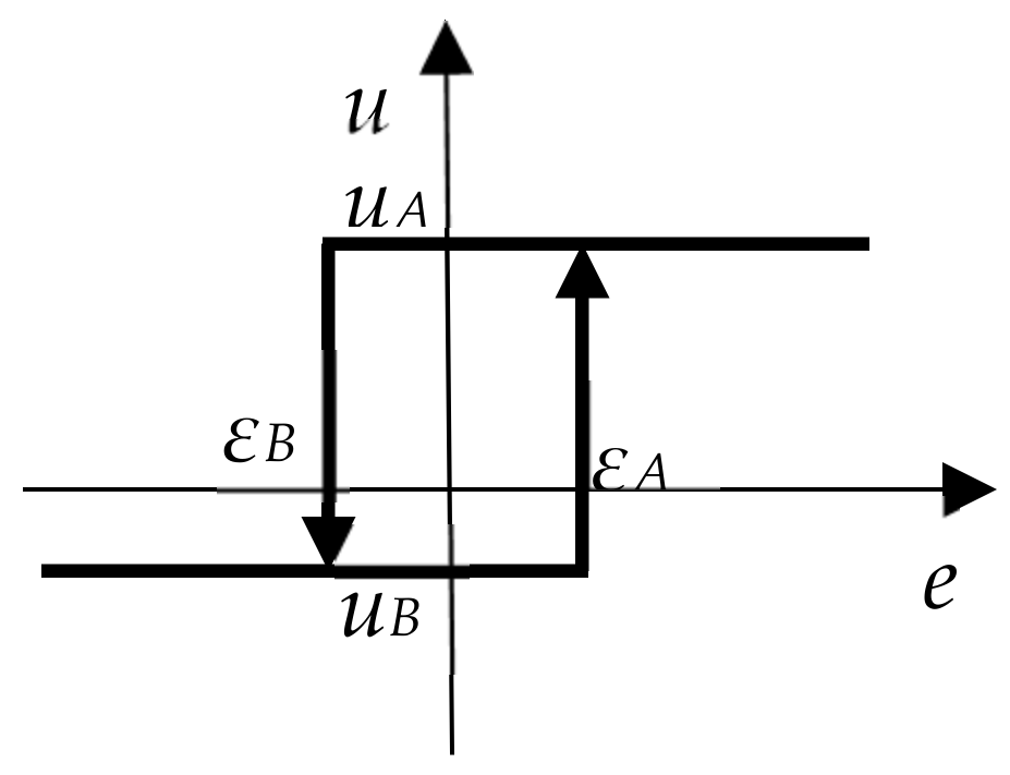
2. Relay Shifting Method

Background

Let us consider a time-invariant process that can be described by the frequency response function G_P(jω) around its operating point, where j is the imaginary unit and ω is the angular frequency. The process is kept near the operating point by a two-position asymmetric relay; see Figure 1, where y denotes the controlled variable, w is the desired variable, e is the control error and u is the manipulated variable. Figure 2 shows the static characteristics of the relay with hysteresis, where the parameters u_A, u_B are selected so that there is a stable oscillation with the period T_p (T_p = T₁ + T₂, T₁ ≠ T₂) (see Figure 3). The parameters ε_A, ε_B help to reduce the influence of a noisy environment. The hysteresis helps reduce the effects of measurement noise by enabling noiseless control action and increases the period of oscillation. It is recommended to adjust the hysteresis to 2–3 times the noise level [19]. The experimental time corresponds to approximately 3 to 4 periods of T_p [13].

The core of the method consists of a simple calculation of the auxiliary variables u_n(t) and y_n(t), n = 2, 3, …, N from the measured courses y₁(t) ≡ y(t) and u₁(t) ≡ u(t) using the following relations:

$$u_n\left(t\right)={\displaystyle \sum _{k=0}^{n-1}{u}_1\left(t-k\frac{T_P}{n}\right)}$$

(1)

$$y_n\left(t\right)={\displaystyle \sum _{k=0}^{n-1}{y}_1\left(t-k\frac{T_P}{n}\right)}$$

(2)

The calculated variables y_n(t) and u_n(t), n = 2, 3, …, N are periodic with the period T_P/n if the measured variables u₁(t) and y₁(t) are periodic with the period T_P. In our case, we assume t > t_L, where t_L is the time when the stable oscillation is achieved. In Figure 4, the time courses of the measured variables u₁(t) and y₁(t) are depicted together with the calculated variables y_n(t) and u_n(t), n = 2, 3 for illustration. The relationships (1) and (2) describe the shifting filter with the following frequency transfer function:

$$F_n\left(j\omega \right)={\displaystyle \sum _{k=0}^{n-1}{e}^{-j\omega \cdot k\cdot \frac{T_p}{n}}}$$

(3)

and it holds.

$$F_n\left(j\omega \right)=〈\begin{array}{c}n\hspace{1em}\mathrm{for} \omega =n\cdot 2\pi /T_P\hspace{1em}\hspace{1em}\\ 0\hspace{1em}\mathrm{for} \omega =k\cdot 2\pi /T_P,k=1,2,\cdots ,n-1\end{array}$$

(4)

The shifting filter F_n filters out lower harmonics and amplifies the n-th harmonic.

The frequency response points G(jω_k), k = 1, 2, …, N can be determined by one of the following procedures ((a) or (b)):

(a)

$$G\left(j{\omega }_k\right)=\frac{{\displaystyle \underset{t}{\overset{t+T_P}{\int }}{y}_k\left(\tau \right)e^{-j{\omega }_k\tau }d\tau }}{{\displaystyle \underset{t}{\overset{t+T_P}{\int }}{u}_k\left(\tau \right)e^{-j{\omega }_k\tau }d\tau }},t>t_L,k=1,2,\cdots ,N$$

(5)

where

$${\omega }_k=k\cdot \frac{2\pi }{T_P}$$

(6)

The integrals in the numerators are calculated by numerical integration. The great advantage of the relay shifting method is that without assuming any model structure, it is possible to estimate the frequency response points G(jω_k), k = 1, 2, …, N from a single relay test.

(b) The position G(jω_k) can also be determined without the utilization of Relation (5) using the approximation of the periodic signals u_k(t) and y_k(t) for k = 1, 2, …, N, t > t_L by harmonic functions and by determining their amplitude ratio and phase shift (see [17] for example).

The real and imaginary parts (Re[G(jω_k)] and Im[G(jω_k)]) or the amplitude ratio |G(jω_k)| and the phase shift arg(G(jω_k)) determine two conditions for each frequency response point G(jω_k). This gives us 2N conditions for fitting a model from N frequency response points G(jω_k), k = 1, 2, …, N.

If we know the static gain K of a proportional system, then the frequency response point G(0) is determined too. This point can also be estimated from a single relay test by the following formula (see [6,20]) if the operating point (u₀,y₀) is known since the shifting method uses the biased relay.

$$G\left(0\right)=K=\frac{{\displaystyle \underset{t}{\overset{t+T_p}{\int }}\left(y\left(\tau \right)-y_0\right)d\tau }}{{\displaystyle \underset{t}{\overset{t+T_p}{\int }}\left(u\left(\tau \right)-u_0\right)d\tau }},t>t_L$$

(7)

3. Model Fitting

Let us assume that a process can be described by a model transfer function, as follows:

$$M\left(s\right)=\frac{b_0+b_{1}s+\dots +b_m{s}^m}{a_0+a_{1}s+\dots a_n{s}^n}\cdot e^{-s{T}_d},n\ge m$$

(8)

where s is the complex variable in the Laplace transform, a₀, a₁, …, a_n, b₀, b₁, …, b_m $\in \mathbb{R}$, and T_d is a transport delay. Then the parameters a₀, a₁, …, a_n, b₀, b₁, …, b_m, and T_d can be estimated using the frequency response points G(jω_k), k = 1, 2, …, N by iterative calculation if the selected value of N is ≥(n + m + 3)/2. If the process is at a steady state, we can obtain the time delay from the initial output response to the relay test and determine the other parameters by the least-squares method (LSM), for example, [21]. The LSM can also be used for parameter fitting if a rational (Padé) approximation of the transport delay term is substituted.

The previous theoretical result is not directly usable for practical applications because we must consider the initial conditions, the precision of measurement, the position of the frequency response points, the choice of the linear model structure, the influence of disturbances, numerical aspects, and so on.

Our goal was to find a mathematical model that will be used to design a PID controller. For this purpose, we used a second-order time-delayed (SOTD) model with a transfer function.

$$M\left(s\right)=\frac{K\cdot e^{-s\cdot T_d}}{a_2{s}^2+a_{1}s+1}$$

(9)

The SOTD model is very versatile and can be used to describe most non-oscillating or oscillating proportional systems with or without a transport delay (see [22,23]). This model has only four parameters—a₂, a₁, K, and T_d, which can be estimated from the frequency response points G(0) and G(jω_k), k = 1, 2, …, N. The model parameters can be estimated by

$$\widehat{\theta }=\underset{\theta \in \Theta }{\arg \min }Kr\left(\theta \right)$$

(10)

where the vector of model parameters

$$\theta ={[K\hspace{0.33em}{a}_2\hspace{0.33em}{a}_1\hspace{0.33em}\tau ]}^T$$

(11)

Θ is the set of acceptable values of the model parameters. For a stable system,

$$\Theta =\left\{\left(K,a_2,a_1,\tau \right):K>0,a_2>0,a_1>0,\tau \in 〈0,{\tau }_m〉\right\}$$

(12)

τ_m is the maximum possible transport delay (see Figure 3) and “T” denotes the transpose operator.

By denoting the real and imaginary part of the complex values G(jω_i),

$$G\left(j{\omega }_i\right)=R_i+I_i\cdot j,\hspace{0.33em}\mathrm{for} i=1,2,\cdots ,N$$

(13)

Then,

$$\widehat{\theta }=\underset{\begin{array}{l}\tau =0,\Delta \tau ,\cdots ,{\tau }_m\\ K,\hspace{0.17em}{a}_2,a_1>0\end{array}}{\arg \min }Kr\left(\left[\begin{array}{c}{\left(Z^{T}Z\right)}^{-1}\cdot Z^{T}p\\ \tau \end{array}\right]\right)$$

(14)

where Δτ is the selected accuracy of the estimation τ,

$$Z=\left[\begin{array}{c}\begin{array}{ccc}\begin{array}{c}\cos {\omega }_1\tau \\ -\sin {\omega }_1\tau \\ \cos {\omega }_2\tau \\ -\sin {\omega }_2\tau \end{array}& \begin{array}{c}{R}_1{\omega }_1^2\\ I_1{\omega }_1^2\\ R_2{\omega }_2^2\\ I_2{\omega }_2^2\end{array}& \begin{array}{c}{I}_1{\omega }_1\\ -R_1{\omega }_1\\ I_2{\omega }_2\\ -R_2{\omega }_2\end{array}\end{array}\\ \begin{array}{ccc}⋮& ⋮& ⋮\\ \cos {\omega }_N\tau & R_N{\omega }_N^2& I_N{\omega }_N\\ -\sin {\omega }_N\tau & I_N{\omega }_N^2& -R_N{\omega }_N\end{array}\end{array}\right],p=\left[\begin{array}{c}{R}_1\\ I_1\\ R_2\\ I_2\\ ⋮\\ \begin{array}{c}{R}_N\\ I_N\end{array}\end{array}\right],$$

(15)

the matrix Z is assumed with the maximum column rank. In this way, we can estimate the model parameters from 2N equations (generalization in comparison with [24]). A similar approach can also be used for fitting linear models with more parameters. The proposed procedure, unlike that of [15], does not require the solution of a system of nonlinear equations and is also applicable to the identification of underdamped systems.

Model (15) has four parameters and, therefore, only two frequency response points are sufficient for the parameter estimation (N = 2). In case we know the values of some parameters, for example, the steady-state gain or the dead time, the number of estimated parameters will be reduced, and a similar approach may be used.

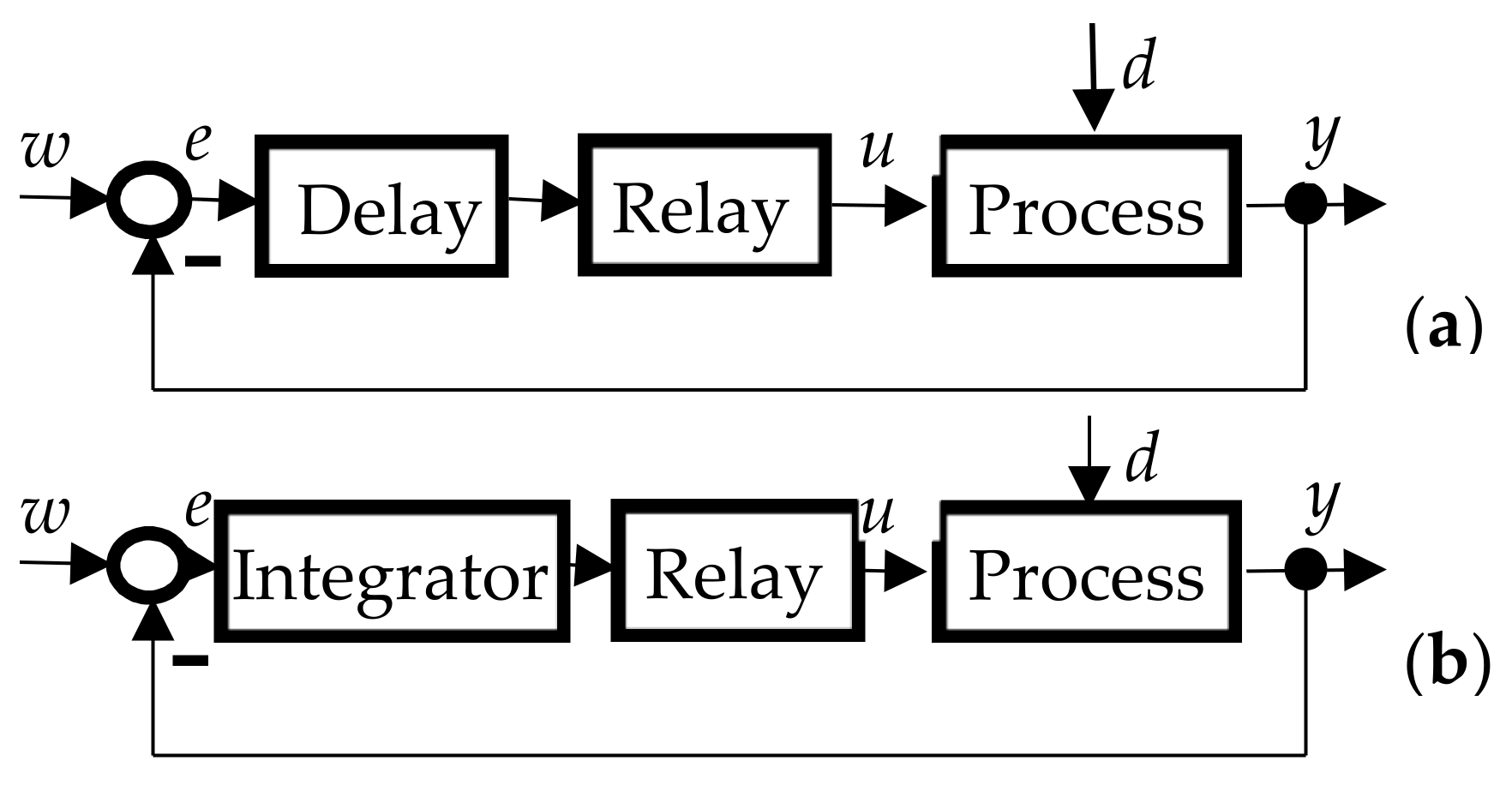
4. Relay Shifting Method with Additional Delay or Integrator

Using the shifting method, we obtained the frequency response points for higher frequencies. We know from classical control theory that the values of the process transfer function for PID tuning are decisive in the range where the phase delay is from 0° to 180° and, consequently, for lower frequencies. To get the frequency response points for lower frequencies, we used an additional integrator or a delay (see Figure 5).

The additional integrator or the delay can be used only if a steady-state oscillation can be achieved with the relay feedback control. To a certain extent, the frequencies of the obtained frequency response points can also be reduced by increasing the relay hysteresis.

5. Examples of Using the Relay Shifting Method

In this section, several different types of processes are identified using the relay shifting method. The proportional processes are modeled by transfer function (9) and the integrating process is modelled by transfer function (16).

$$M\left(s\right)=\frac{1}{s\left(a_{2}s+a_1\right)}\cdot e^{-s\cdot T_d}$$

(16)

In all the simulated examples, we chose N = 2 for the parameter estimation and the biased relay had the following parameters (see Figure 2).

u_A = 2, u_B = −1, ε_A = 0.1, ε_B = −0.1.

(17)

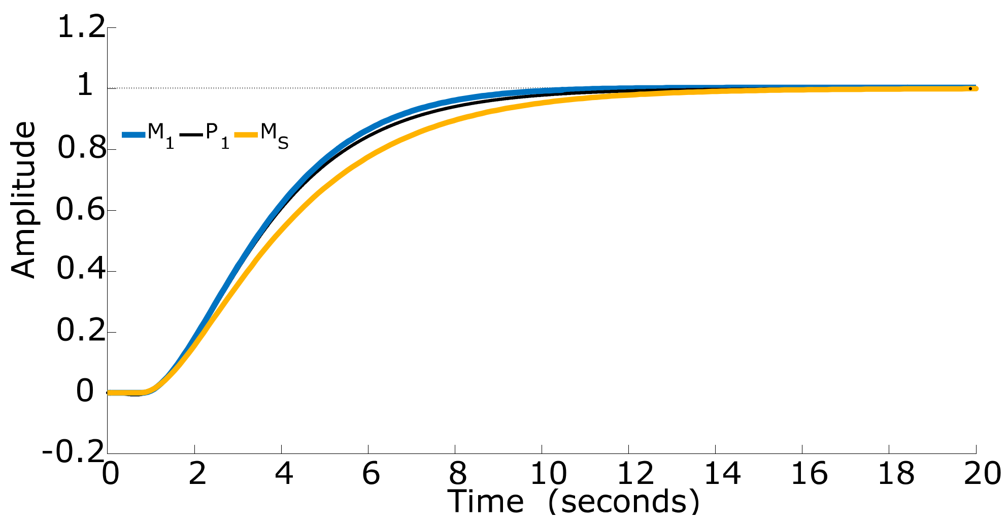
5.1. Lag-Dominated Non-Oscillatory Proportional Process

The lag-dominated non-oscillatory proportional process considered in [22] is given by the following transfer function:

$$P_1\left(s\right)=\frac{\left(-0.3s+1\right)\left(0.08s+1\right)}{\left(2s+1\right)\left(1s+1\right)\left(0.4s+1\right)\left(0.2s+1\right){\left(0.05s+1\right)}^3}$$

(18)

The process is controlled by a relay (see Figure 1). The relay output u and the process output y are depicted in Figure 6.

Using the relay shifting method, we can determine from the observed stable courses u and y that

$$T_P=6.23\mathrm{s},$$

(19)

$$G\left(0\right)=K=1.003,$$

(20)

$$G\left(j{\omega }_1\right)=-0.2845-0.0847j,\hspace{0.33em}G\left(j{\omega }_2\right)=-0.0444+0.0782j,$$

(21)

$${\tau }_m=2.5\mathrm{s},$$

(22)

and the SOTD model, estimated according to Section 2 and Section 3, is

$$M_1\left(s\right)=\frac{1.003\cdot \exp (-0.81s)}{2.511s^2+3.002s+1}$$

(23)

The Nyquist frequency responses of process P₁(s) and model M₁(s) are shown in Figure 7. In the same figure, model M_S(s) and the points G(0), G(jω₁), and G(jω₂) are depicted as well, where

$$M_S\left(s\right)=\frac{\exp \left(-0.77s\right)}{\left(2s+1\right)\left(1.2s+1\right)}$$

(24)

The model M_S(s) was derived by Skogestad [22] directly from (18) using the half rule.

The unit step responses of process P₁(s), model M₁(s), and model M_S(s) are shown in Figure 8.

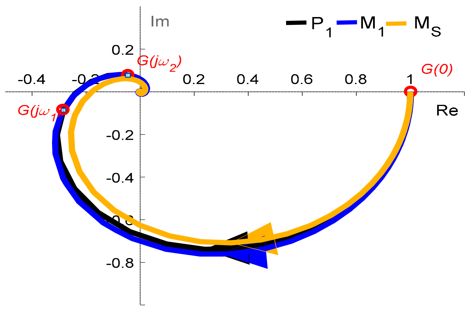
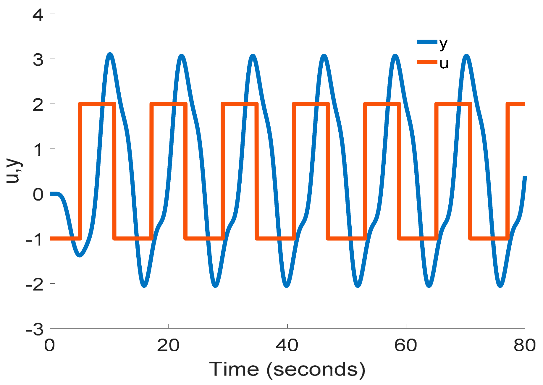
5.2. Lag-Dominated Oscillatory Proportional Process

The lag-dominated oscillatory proportional process considered in [23] is given by the following transfer function:

$$P_2\left(s\right)=\frac{125}{{\displaystyle \prod _{l=1}^4\left(s^2+2{\xi }_l{\omega }_{nl}+{\omega }_{{}_{nl}}^2\right)}}$$

(25)

where ξ₁ = 0.5, ω_n1 = 1.1180, ξ₂ = 0.6, ω_n2 = 2.2361, ξ₃ = 0.65, ω_n3 = 3.1623, ξ₄ = 0.5, and ω_n4 = 1.4142.

The process is controlled by a relay (see Figure 1). The relay output u and the process output y are depicted in Figure 9.

Using the relay shifting method, we can determine from the observed stable courses u and y that

$$T_P=6.44s,$$

(26)

$$G\left(0\right)=K=0.996,$$

(27)

$$G\left(j{\omega }_1\right)=-1.5214-0.0457j,\hspace{0.33em}G\left(j{\omega }_2\right)=0.1863-0.1504j,$$

(28)

$${\tau }_m=2.8s,$$

(29)

and the SOTD model, estimated according to Section 2 and Section 3, is

$$M_2\left(s\right)=\frac{0.996\cdot \exp \left(-2.1s\right)}{0.8855s^2+0.5857s+1}$$

(30)

The Nyquist frequency responses of process P₂(s) and model M₂(s) are shown in Figure 10. In the same figure, the model M_R(s) and the points G(jω₁) and G(jω₂) are depicted as well, where

$$M_R\left(s\right)=\frac{1.198\exp \left(-2.048s\right)}{s^2+0.7691s+1.198}$$

(31)

The model M_R(s) was derived by Novella-Rodriguez et al. [23] directly from (25).

If we use an additional delay or an integrator (see Figure 5), we can receive better positions of the points G(jω₁) and G(jω₂) for the model fitting. In case we use the additional delay D = 3 s, we obtain the time courses u and y depicted in Figure 11.

Using the relay shifting method, we can determine from the observed stable courses u and y that

$$T_P=11.3\mathrm{s},$$

(32)

$$G\left(0\right)=K=0.9995,$$

(33)

$$G\left(j{\omega }_1\right)=0.2304-1.2044j,\hspace{0.33em}G\left(j{\omega }_2\right)=-1.4257+0.4441j,$$

(34)

$${\tau }_m=11.3\mathrm{s},$$

(35)

and the SOTD model, estimated according to Section 2 and Section 3, is

$$M_{2D}\left(s\right)=\frac{0.9995\exp \left(-1.79s\right)}{0.9092s^2+0.6426s+1}$$

(36)

The Nyquist frequency responses of process P₂(s), model M_2D(s), model M_R(s), and points G(jω₁) and G(jω₂) are shown in Figure 12.

The unit step responses of process P₂(s) and models M₂(s), M_2D(s), and M_R(s) are shown in Figure 13.

5.3. Delay-Dominated Non-Oscillatory Proportional Process

The delay-dominated non-oscillatory proportional process considered in [11] (p. 165) is given by the following transfer function:

$$P_3\left(s\right)=\frac{\exp \left(-4s\right)}{{\left(0.5s+1\right)}^3}$$

(37)

The process is controlled by a relay (see Figure 1). The relay output u and the process output y are depicted in Figure 14.

Using the relay shifting method, we can determine from the observed stable courses u and y that

$$T_P=10.90\mathrm{s},$$

(38)

$$G\left(0\right)=K=1.002,$$

(39)

$$G\left(j{\omega }_1\right)=-0.8872+0.0079j,\hspace{0.33em}G\left(j{\omega }_2\right)=0.6472-0.0631j,$$

(40)

$${\tau }_m=4.5\mathrm{s},$$

(41)

and the SOTD model, estimated according to Section 2 and Section 3, is

$$M_3\left(s\right)=\frac{1.002\cdot \exp \left(-4.23s\right)}{0.4513s^2+1.287s+1}$$

(42)

The Nyquist frequency responses of process P₃(s) and model M₃(s) are shown in Figure 15. In the same figure, the model M_LG(s) and the points G(jω₁) and G(jω₂) are depicted as well, where

$$M_{LG}\left(s\right)=\frac{1.000\cdot \exp \left(-4.2771s\right)}{{\left(0.6183s+1\right)}^2}$$

(43)

The model M_LG(s) was derived by Liu and Gao [11] (p. 165) with algorithm RS-SU1.

The unit step responses of process P₃(s), model M₃(s), and model M_LG(s) are shown in Figure 16.

5.4. Integrating Process

The integrating process considered by Liu and Gao [11] (p. 212) is given by the following transfer function:

$$P_4\left(s\right)=\frac{\left(-s+1\right)}{s{\left(s+1\right)}^5}\exp \left(5s\right)$$

(44)

The process is controlled by a relay (see Figure 1). The relay output u and the process output y are depicted in Figure 17.

Using the relay shifting method, we can determine from the observed stable courses u and y that

$$T_P=50.1s,$$

(45)

$$G\left(j{\omega }_1\right)=-7.591-1.451j,\hspace{0.33em}G\left(j{\omega }_2\right)=-1.375+3.250j$$

(46)

$${\tau }_m=13.0s,$$

(47)

and the estimated model is

$$M_4\left(s\right)=\frac{\exp \left(-8.97s\right)}{s\left(2.117s+0.9971\right)}$$

(48)

The Nyquist frequency characteristics of process P₄(s) and model M₄(s) are shown in Figure 18. In the same figure, the model M_4LGI(s) and the points G(jω₁) and G(jω₂) are depicted as well, where

$$M_{4LGI}\left(s\right)=\frac{1.018\exp \left(-8.5278s\right)}{s\left(2.5293s+1\right)}$$

(49)

The model M_4LGI(s) was derived by Liu and Gao [11] (p. 212) with algorithm RI-S1.

The unit step responses of process P₄(s), model M₄(s), and model M_4LGI(s) are shown in Figure 19.

5.5. Unstable Process with Delay

The same approach can be used for unstable processes if there is sustained oscillation in an asymmetric relay feedback test. The unstable process with delay considered by Liu and Gao [11] (p. 235) is given by the following transfer function:

$$P_5\left(s\right)=\frac{1}{\left(5s-1\right)\left(2s+1\right)\left(0.5s+1\right)}{e}^{-0.5s}$$

(50)

This unstable process is controlled by the biased relay where

u_A = 2, u_B = −1.7, ε_A = 0.1, ε_B = −0.1

(51)

(see Figure 2). The relay output u and the process output y are depicted in Figure 20.

From these time courses, we can determine by the shifting method,

$$T_P=24.5s,$$

(52)

$$G\left(j{\omega }_1\right)=-0.5335-0.0931j,\hspace{0.33em}\hspace{0.33em}G\left(j{\omega }_2\right)=-0.2539+0.0278j$$

(53)

$${\tau }_m=5.6s.$$

(54)

The estimated model is

$$M_5\left(s\right)=\frac{0.9983\exp \left(-0.95s\right)}{9.998s^2+2.831s-1}$$

(55)

The Nyquist frequency characteristics of process P₅(s) and model M₅(s) are shown in Figure 21. In the same figure, the model M_5LG(s) and the points G(jω₁) and G(jω₂) are depicted as well, where

$$M_{5LG}\left(s\right)=\frac{1.001\exp \left(-0.94s\right)}{\left(4.9996s-1\right)\left(2.07s+1\right)}$$

(56)

The model M_5LG(s) was derived in [11] (p. 235) with algorithms RU-SA and RU-SB, which result in very similar models.

The unit step responses of process P₅(s), model M₅(s), and model M_5LG(s) are shown in Figure 22.

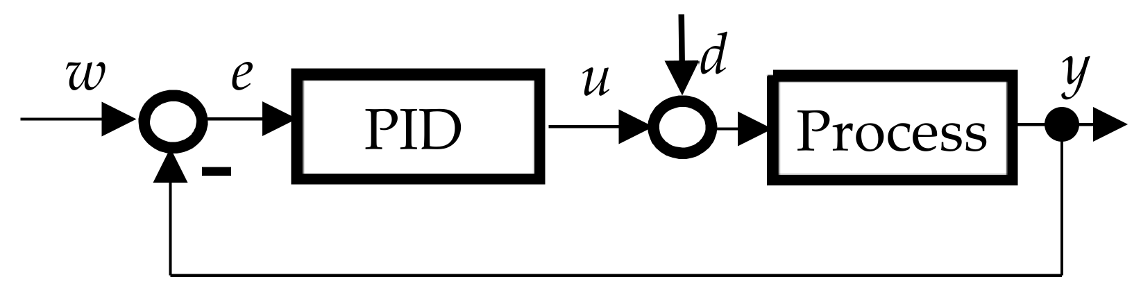
6. PID Controller Tuning

If we know the process model, we need to determine the parameters of the controller. There are a number of recommendations for PID controller tuning that can be used for control of a process described by transfer function (9) (see, for example, Åström and Hägglund [25], Skogestad and Grimholt [26], Novella-Rodriguex et al. [23], and O’Dwyer [27]).

We can also use the following tuning rules, which are very simple, and they should work well on a wide range of stable processes (non-oscillatory/oscillatory, lag/delay dominated) described by process model (9).

Let the transfer function of the ideal PID controller be

$$C\left(s\right)=r_P+\frac{r_I}{s}+r_D\cdot s$$

(57)

where r_P,r_I, and r_D are adjustable controller parameters.

The open-loop transfer function is

$$\begin{array}{c}{G}_o\left(s\right)=C\left(s\right)\cdot M\left(s\right)=\\ =\frac{rI\left(\frac{r_D}{r_I}\cdot s^2+\frac{r_P}{r_I}\cdot s+1\right)}{s}\cdot \frac{K\exp \left(-s\cdot T_d\right)}{a_2{s}^2+a_{1}s+1}\end{array}$$

(58)

If we choose

$$\frac{r_D}{r_I}=a_2,\hspace{0.33em}\frac{r_P}{r_I}=a_1$$

(59)

then

$$G_o\left(s\right)=\frac{r_I\cdot K\cdot \exp \left(-s{T}_d\right)}{s}$$

(60)

and the closed-loop transfer function is

$$G_{wy}\left(s\right)=\frac{G_o\left(s\right)}{1+G_o\left(s\right)}=\frac{r_I\cdot K\cdot \exp \left(-s{T}_d\right)}{s+r_{I}K\exp \left(-s{T}_d\right)}$$

(61)

The parameter r_I can be determined by the Nyquist stability criterion using the open-loop transfer function (60) and by a choice of the gain margin m_A or the phase margin γ. For common control systems, the recommended values are as follows (see, for example, Víteček and Vítečková [28], and Landau and Zito [29]):

$$m_A\in 〈2,5〉,\hspace{0.33em}\gamma \in 〈\pi /6,\pi /3〉.$$

(62)

With this approach, we can easily derive that

$$r_I=\frac{\pi }{2\cdot T_d\cdot m_A\cdot \left|K\right|}$$

(63)

and

$$r_I=\frac{\pi -2\gamma }{2\left|K\right|\cdot T_d}$$

(64)

The value of the parameter r_I can also be chosen according to the denominator Q(s) of the control transfer function (61). The characteristic equation of the control system has the transcendental form

$$Q\left(s\right)=s+r_{I}K\exp \left(-s{T}_d\right)=0.$$

(65)

The control system is stable for

$$r_I<\frac{\pi }{2\left|K\right|T_d}$$

(66)

This equation also follows from (63) and (64) for m_A = 1 and γ = 0. With the parameter r_I, we can change the behavior of the closed-loop system. The value of the parameter r_I can be chosen, for example, from the characteristic Equation (65) to obtain the double real dominant pole s_1,2. This pole can be determined from Equation (65) and the following equation:

$$\frac{dQ\left(s\right)}{ds}=0=1+r_{I}K\exp \left(-s{T}_d\right)\cdot \left(-T_d\right)$$

(67)

From (65) and (67), it follows

$$s_{1,2}=-\frac{1}{T_d}$$

(68)

and

$$r_I=\frac{1}{K\cdot \exp \left(1\right)\cdot T_d}$$

(69)

By comparing, for example, (63) and (69), it is obvious that the adjustment according to (69) corresponds to the gain margin m_A = 4.27.

To summarize the presented results for PID tuning so far, at first, we determine the parameter r_I (using one of the relations (63) or (64)), and then we determine using relation (59)

$$r_P=a_1\cdot r_I,$$

(70)

$$r_D=a_2\cdot r_I.$$

(71)

The resulting relationships for adjusting the PID controller are computationally simple and easily understandable; they are not based on the approximation of the transport delay and are usable for stable oscillatory or non-oscillatory systems.

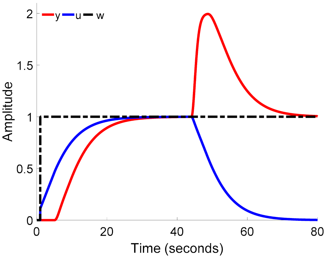
7. Examples of PID Tuning to Control Stable Processes Identified by the Relay Shifting Method

In all examples, the parameter r_I was estimated according to relation (69), and the parameters r_P, r_D by relations (70), (71). The PID control was applied directly to the original processes, and the models, obtained by the relay shifting method, were used only for the PID tuning. The processes were controlled by the PID 2DOF controller which is described by

$$U\left(s\right)=r_{P}E\left(s\right)+r_I\cdot \frac{E\left(s\right)}{s}-r_{D}s\frac{Y\left(s\right)}{\frac{1}{N}s+1}$$

(72)

where U(s), E(s), and Y(s) are the Laplace images of u(t), e(t), and y(t), respectively. The PID 2DOF controller eliminates “derivative kick” and is less sensitive to measurement noise. In all examples, the parameter N = 10.

Let us consider the closed-loop system given in Figure 23. The simulated unit step responses of closed-loop control systems for setpoints w and change of load disturbances d are shown in the following examples.

7.1. PID Control of Process P₁

The model M₁ (23) of the process P₁ (18) was obtained by the relay shifting method. The relations (69)–(71) determine the parameters r_I, r_P, and r_D of the PID controller, respectively.

$$r_I=\frac{1}{K\cdot \exp \left(1\right)\cdot T_d}=\frac{1}{1.003\cdot \exp (1)\cdot 0.81}=0.4528$$

(73)

$$r_P=a_1\cdot r_I=3.002\cdot 0.4528=1.3593,$$

(74)

$$r_D=a_2\cdot r_I=2.511\cdot 0.4528=1.1370.$$

(75)

The unit step responses y of the closed-loop control system for the setpoint change w and the change of load disturbance d are shown in Figure 24. The unit step of the load disturbance d was at the time t = 20 s.

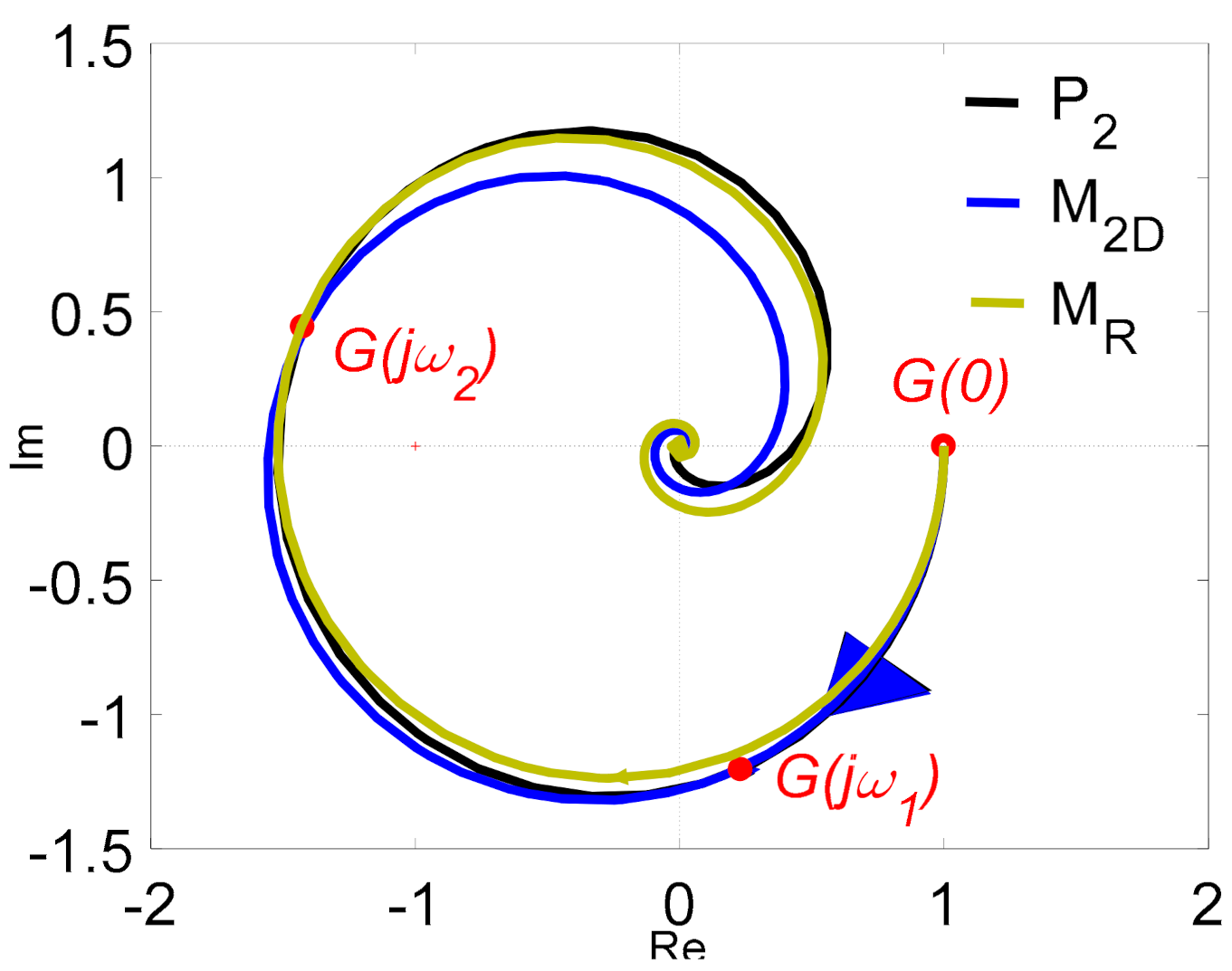
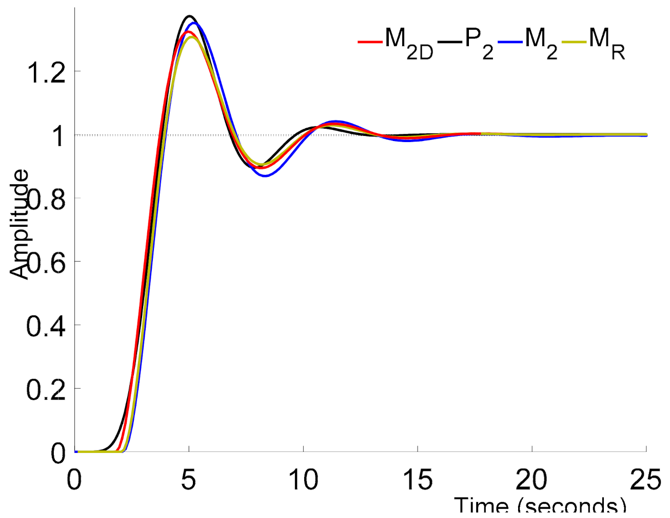
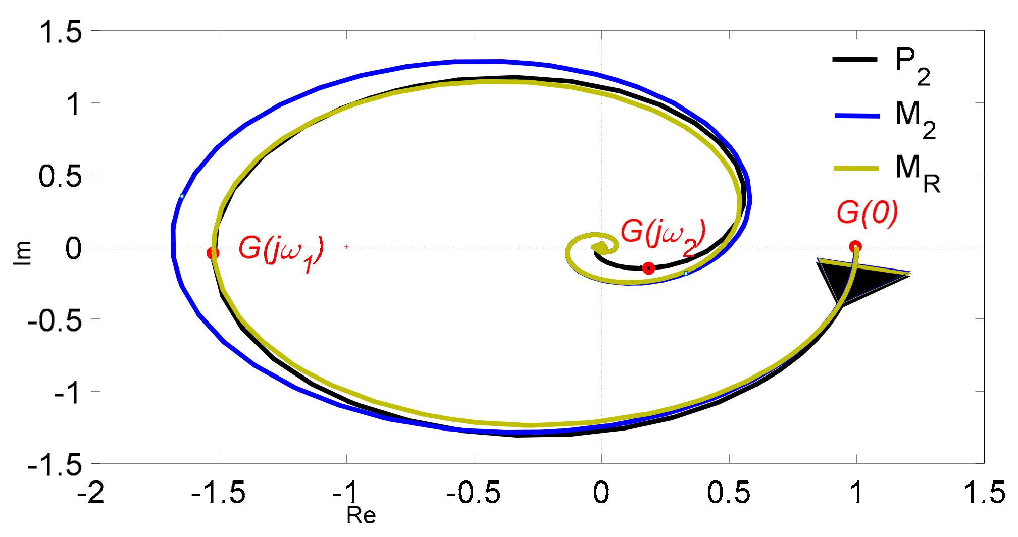
7.2. PID Control of Process P₂

The model M₂ (30) of the process P₂ (25) was obtained by the relay shifting method. The relations (69)–(71) determine the parameters r_I, r_P, and r_D of the PID controller, respectively.

$$r_I=\frac{1}{K\cdot \exp \left(1\right)\cdot T_d}=\frac{1}{0.996\cdot \exp (1)\cdot 2.1}=0.1759,$$

(76)

$$r_P=a_1\cdot r_I=0.5857\cdot 0.1759=0.1030,$$

(77)

$$r_D=a_2\cdot r_I=0.8855\cdot 0.1759=0.1558.$$

(78)

The controlled variables y for the setpoint change w and the change of load disturbance d are shown in Figure 25. The unit step of the load disturbance d was at the time t = 40 s.

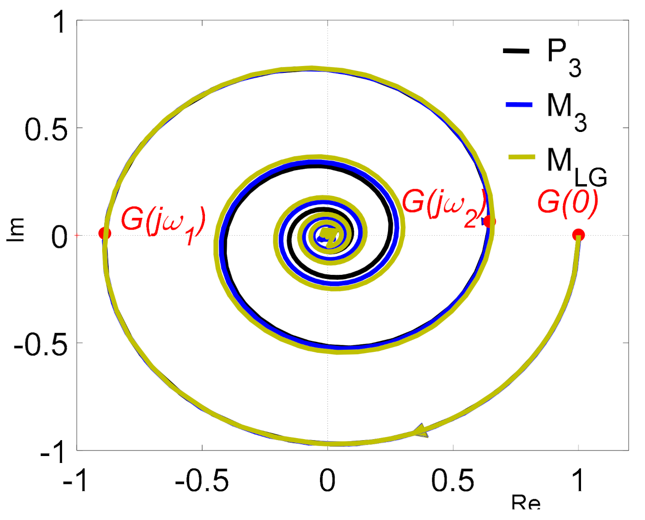
7.3. PID Control of Process P₃

The model M₃ (42) of the process P₃ (37) was obtained by the relay shifting method. The relations (69), (70), and (71) determine the parameters r_I, r_P, and r_D of the PID controller.

$$r_I=\frac{1}{K\cdot \exp \left(1\right)\cdot T_d}=\frac{1}{1.002\cdot \exp (1)\cdot 4.23}=0.0868$$

(79)

$$r_P=a_1\cdot r_I=1.287\cdot 0.0868=0.1117,$$

(80)

$$r_D=a_2\cdot r_I=0.4513\cdot 0.0868=0.0392.$$

(81)

The unit step responses y of the closed-loop control system for the setpoint change w and the change of load disturbance d are shown in Figure 26. The unit step of the load disturbance d was at the time t = 40 s.

8. Verification and Implementation

The proposed identification method for PID tuning was tested on both simulation examples and on real laboratory apparatuses, namely “Water Levitation”, “Air Aggregate”, and “Air Levitation” (see [30,31]), and the results of the relay shifting method were compared with the results of other identification approaches to verify the practical benefits of the use of this method in the work by Hornychová and Hofreiter [32]. The experiments were realized both in the Matlab/Simulink environment and physically, using the industrial PLC Tecomat Foxtrot produced by TECO a.s. (see TECO Advanced Automation [33]). The comprehensive development tool Mosaic was used for writing and debugging the relay identification and PID tuning programs for the PLC Tecomat Foxtrot (see Vaněk and Slabý [34]).

9. Conclusions

The presented relay shifting method has the following properties:

• The frequency points G(jω_i), i = 1, 2,$\cdots ,$ N are determined from one relay feedback test without any prior knowledge of the model.

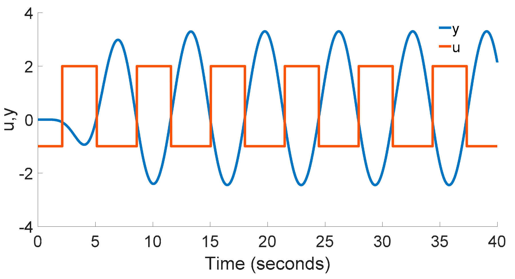
• The relay shifting method is very versatile, the same procedure can be used for the model parameter estimation of stable/unstable/integrating, non-oscillatory/oscillatory, and lag/delay dominated processes and the noisy environment if there are stable oscillations for the relay feedback test.
• The static load disturbance has no effect on the locations of the frequency points G(jω_i), i = 1, 2,$\cdots ,$ N.

• By using the SOTD model, it is possible to estimate the steady-state gain even in the presence of a constant load disturbance.
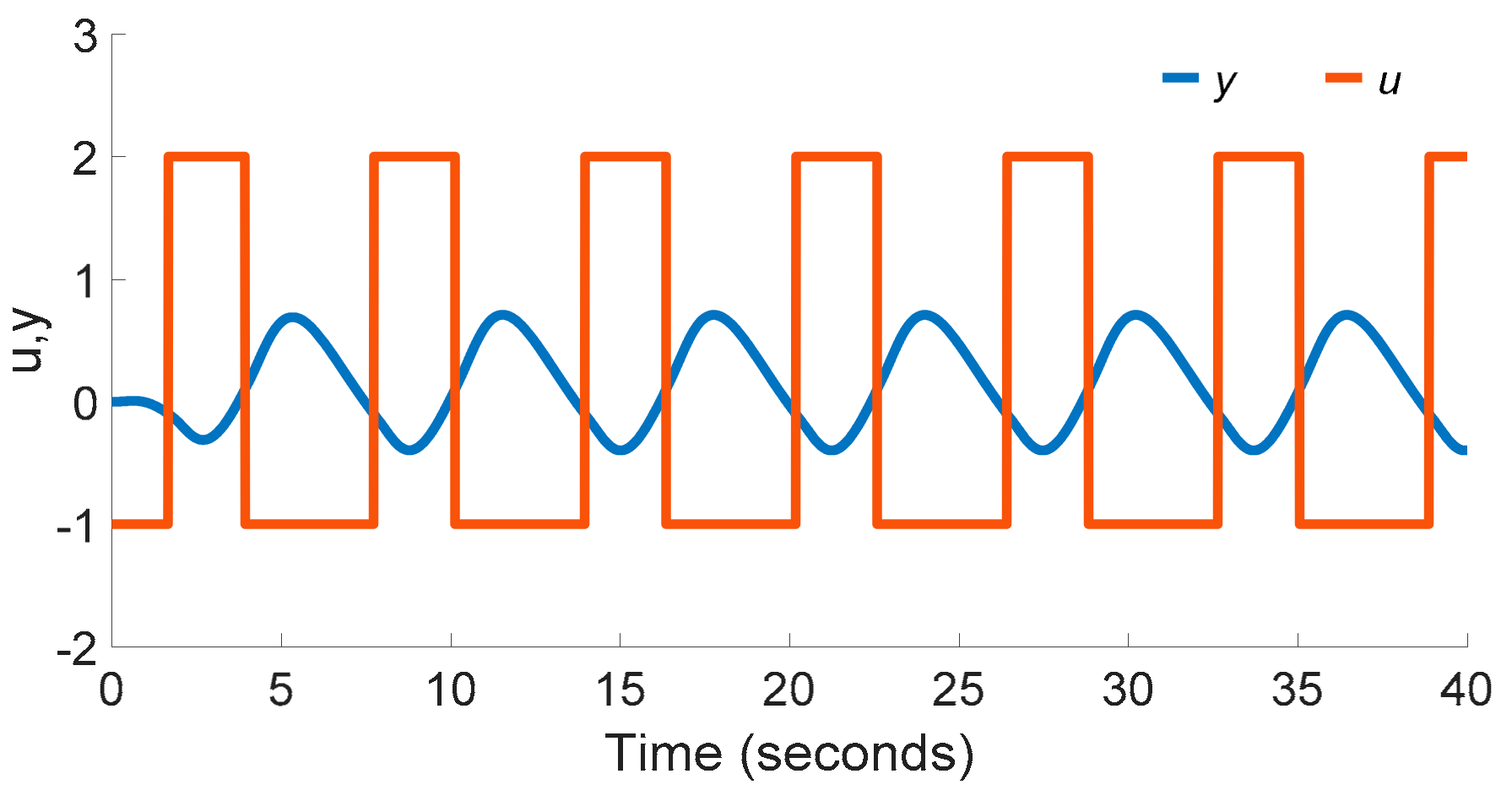
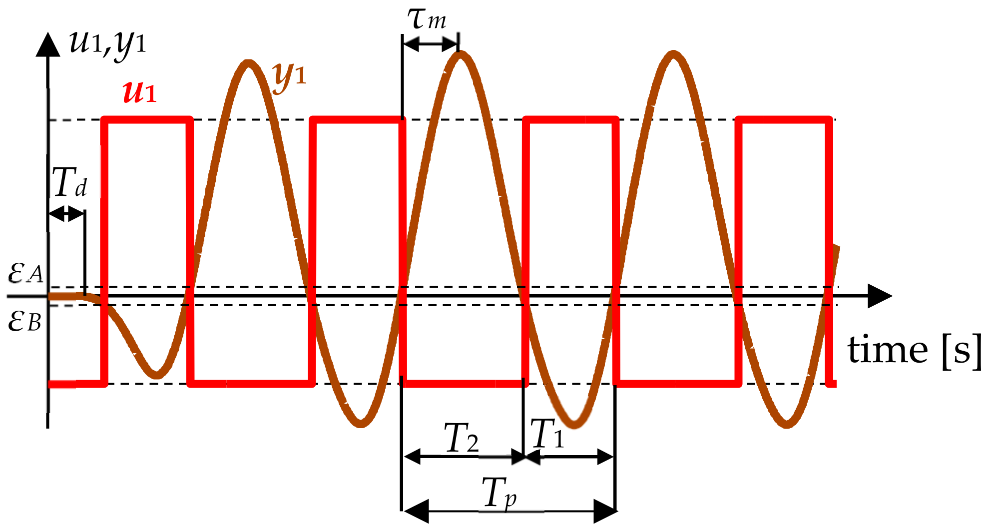
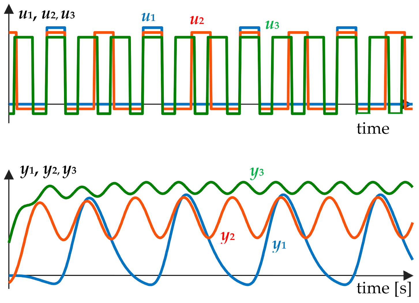
• The shifting filter described by (1) and (2) filters out the lower harmonics and amplifies the n-th harmonic, and the frequency response point G(jω_n) can be determined by relation (5) or by using the approximation of the periodic signals u_n(t) and y_n(t) by harmonic functions.
• The relay shifting filter helps to eliminate parasitic signals.
• The relay shifting method is appropriate only for processes describable by linear time-invariant models.
• The position of the points G(jω_i), i = 1, 2, …, N significantly affects the estimation of the model parameters. An additional integrator or a delay helps to improve the parameter estimation.
• Using the SOTD model, it is possible to model processes that can be described by high-order models.
• The relay shifting method is primarily suggested for the automatic tuning of controllers.

The combination of the shifting method and the additional delay or the additional integrator in the relay feedback loop allows for the estimation of the frequency response points G(jω_k), k = 1, 2, …, N, from a single relay test. To obtain more frequency response points, we can select different values of the additional delay or the integral gain of the additional integrator for each relay feedback test. This approach makes it possible to acquire other frequency response points.

In this paper, we have summarized the relay shifting method that can be used for estimating the parameters of simpler and more complex linear models with different structures describing systems where steady oscillations can be achieved by means of relay control. We presented a simple original algorithm for estimating the parameters of the SOTD model from N points of the frequency response. The relay shifting method for open-loop stable, unstable, and integration processes, even with a delay, and regardless of whether they are oscillating or non-oscillating, was demonstrated by simulation examples. The article also introduced the design and simulation testing of a simple PID controller adjustment for the control of a stable system described by an SOTD model without using the delay approximation.

References

1. Rotač, V.J. Rasčet Nastrojki Promyšlenych Sistem Regulirovanija; Gosenergoizdat: Moskva, Russia, 1961. [Google Scholar]
2. Åström, K.J.; Hägglund, T. Automatic Tuning of Simple Regulators with Specifications on Phase and Amplitude Margins. Automatica 1984, 20, 645–651. [Google Scholar] [CrossRef] [Green Version]
3. Khalil, H.K. Nonlinear Systems, 3rd ed.; Prentice Hall: Upper Saddle River, NJ, USA, 2002; ISBN 978-0-13-067389-3. [Google Scholar]
4. Ziegler, J.G.; Nichols, N.B. Optimum Settings for Automatic Controllers. Trans. ASME 1942, 64, 759–768. [Google Scholar] [CrossRef]
5. Luyben, W.L. Derivation of Transfer Functions for Highly Nonlinear Distillation Columns. Ind. Eng. Chem. Res. 1987, 26, 2490–2495. [Google Scholar] [CrossRef]
6. Shen, S.-H.; Wu, J.-S.; Yu, C.-C. Use of Biased-Relay Feedback for System Identification. AIChE J. 1996, 42, 1174–1180. [Google Scholar] [CrossRef]
7. Li, W.; Eskinat, E.; Luyben, W.L. An Improved Autotune Identification Method. Ind. Eng. Chem. Res. 1991, 30, 1530–1541. [Google Scholar] [CrossRef]
8. Bi, Q.; Wang, Q.-G.; Hang, C.-C. Relay-Based Estimation of Multiple Points on Process Frequency Response. Automatica 1997, 33, 1753–1757. [Google Scholar] [CrossRef]
9. Chidambaram, M.; Sathe, V. Relay Autotuning for Identification and Control; Cambridge University Press: Cambridge, UK, 2014; ISBN 978-1-107-41596-6. [Google Scholar]
10. Liu, T.; Wang, Q.-G.; Huang, H.-P. A Tutorial Review on Process Identification from Step or Relay Feedback Test. J. Process. Control 2013, 23, 1597–1623. [Google Scholar] [CrossRef]
11. Liu, T.; Gao, F. Industrial Process Identification and Control Design: Step-Test and Relay-Experiment-Based Methods. In Advances in Industrial Control; Springer: London, UK, 2011. [Google Scholar]
12. Dharmalingam, K.; Thangavelu, T. Parameter Estimation Using Relay Feedback. Rev. Chem. Eng. 2019, 35, 505–529. [Google Scholar] [CrossRef]
13. Yu, C.C. Autotuning of PID Controllers; Springer: London, UK, 2006; ISBN 978-1-84628-036-8. [Google Scholar]
14. Ruderman, M. Relay Feedback Systems—Established Approaches and New Perspectives for Application. IEEJ J. IA 2019, 8, 271–278. [Google Scholar] [CrossRef] [Green Version]
15. Sánchez Moreno, J.; Dormido Bencomo, S.; Díaz Martínez, J.M. Fitting of Generic Process Models by an Asymmetric Short Relay Feedback Experiment—The n-Shifting Method. Appl. Sci. 2021, 11, 1651. [Google Scholar] [CrossRef]
16. Vivek, S.; Chidambaram, M. Identification Using Single Symmetrical Relay Feedback Test. Comput. Chem. Eng. 2005, 29, 1625–1630. [Google Scholar] [CrossRef]
17. Hofreiter, M. Extension of Relay Feedback Identification. In Proceedings of the 2015 7th International Congress on Ultra Modern Telecommunications and Control Systems and Workshops (ICUMT), Brno, Czech Republic, 6–8 October 2015; pp. 61–66. [Google Scholar]
18. Hofreiter, M. Shifting Method for Relay Feedback Identification. IFAC-Pap. 2016, 49, 1933–1938. [Google Scholar] [CrossRef]
19. Berner, J.; Hägglund, T.; Åström, K.J. Asymmetric Relay Autotuning—Practical Features for Industrial Use. Control Eng. Pract. 2016, 54, 231–245. [Google Scholar] [CrossRef]
20. Berner, J.; Hagglund, T.; Astrom, K.J. Improved Relay Autotuning Using Normalized Time Delay. In Proceedings of the 2016 American Control Conference (ACC), Boston, MA, USA, 6–8 July 2016; pp. 1869–1875. [Google Scholar]
21. Seborg, D.E. Process Dynamics and Control, 3rd ed.; John Wiley & Sons, Inc.: Hoboken, NJ, USA, 2011; ISBN 978-0-470-12867-1. [Google Scholar]
22. Skogestad, S. Simple Analytic Rules for Model Reduction and PID Controller Tuning. J. Process. Control 2003, 13, 291–309. [Google Scholar] [CrossRef] [Green Version]
23. Novella-Rodríguez, D.F.; del Muro-Cuéllar, B.; Hernandez-Hernández, G.; Marquez-Rubio, J.F. Delayed Model Approximation and Control Design for Under-Damped Systems. IFAC-PapersOnLine 2017, 50, 1316–1321. [Google Scholar] [CrossRef]
24. Hofreiter, M. Improved Relay Feedback Identification Using Shifting Method. In Proceedings of the 16th International Conference on Informatics in Control, Automation and Robotics, Prague, Czech Republic, 29–31 July 2019; SCITEPRESS—Science and Technology Publications: Prague, Czech Republic, 2019; pp. 601–608. [Google Scholar]
25. Åström, K.J.; Hägglund, T.; Åström, K.J. PID Controllers, 2nd ed.; International Society for Measurement and Control: Research Triangle Park, NC, USA, 1995; ISBN 978-1-55617-516-9. [Google Scholar]
26. Skogestad, S.; Grimholt, C. The SIMC Method for Smooth PID Controller Tuning. PID Control in the Third Millennium: Lessons Learned and New Approaches. In Advances in Industrial Control; Springer: Berlin/Heidelberg, Germany, 2012; pp. 147–175. ISBN 978-1-4471-2424-5. [Google Scholar]
27. O’Dwyer, A. Handbook of PI and PID Controller Tuning Rules, 3rd ed.; Imperial College Press: London, UK, 2009; ISBN 978-1-84816-242-6. [Google Scholar]
28. Víteček, A.; Vítečková, M. Vysoká škola báňská—Technická univerzita Ostrava; Katedra automatizační techniky a řízení. In Closed-Loop Control of Mechatronic Systems; VŠB—Technical University of Ostrava: Ostrava, Czech Republic, 2013; ISBN 978-80-248-3149-7. [Google Scholar]
29. Landau, Y.D.; Zito, G. Digital Control Systems: Design, Identification and Implementation; Springer Science & Business Media: Berlin/Heidelberg, Germany, 2010; ISBN 978-1-84996-551-4. [Google Scholar]
30. Hornychová, A.; Hofreiter, M. Use of the Shifting Method Results for PID Controllers Parameters Estimation. MATEC Web Conf. 2019, 292, 01017. [Google Scholar] [CrossRef]
31. Hofreiter, M. Relay Feedback Identification with Additional Integrator. IFAC-PapersOnLine 2019, 52, 66–71. [Google Scholar] [CrossRef]
32. Hornychova, A.; Hofreiter, M. Relay Feedback Identification Method for PID Controller Tuning. In Proceedings of the 2020 21th International Carpathian Control Conference (ICCC), High Tatras, Slovakia, 27–29 October 2020; pp. 1–6. [Google Scholar]
33. TECO Advanced Automation PLC Tecomat Foxtrot; TECO a.s.: Kolín, Czech Republic, 2021; Available online: https://www.Tecomat.Com/Products/Cat/Cz/Plc-Tecomat-Foxtrot-3/ (accessed on 2 March 2021).
34. Vaněk, J.; Slabý, J. Computing of PID Parameters Using Tecomat Foxtrot and the Asymmetrical Relay Shifting. In Proceedings of the New Methods and Practices in the Instrumentation, Automatic Control and Informatics 2020; CTU in Prague: Lobeč, Czech Republic, 2020; pp. 24–32. [Google Scholar]
Figure 1. A process under relay control.
Energies 14 05945 g001
Figure 2. Static characteristics of an asymmetric relay with hysteresis.
Energies 14 05945 g002
Figure 3. Time courses of the manipulated variable u1 and the controlled variable y1 under relay control.
Energies 14 05945 g003
Figure 4. The time courses of u1 and y1 during the relay feedback control together with calculated u2, y2, u3, y3.
Energies 14 05945 g004
Figure 5. Relay feedback with additional delay (a) and with additional integrator (b).
Energies 14 05945 g005
Figure 6. The relay output u and the observed output y of the process P1(s).
Energies 14 05945 g006
Figure 7. The Nyquist frequency plots of transfer functions P1(s), M1(s), and MS(s).
Energies 14 05945 g007
Figure 8. The unit step responses of process P1(s), model M1(s), and model MS(s).
Energies 14 05945 g008
Figure 9. The relay output u and the observed output y of the process P2(s).
Energies 14 05945 g009
Figure 10. The Nyquist frequency plots of transfer functions P2(s), M2(s), and MR(s).
Energies 14 05945 g010
Figure 11. The relay output u and the observed output y of the process P2(s) controlled by the relay with the additional delay D = 3 s.
Energies 14 05945 g011
Figure 12. The Nyquist frequency plots of transfer functions P2(s), M2D(s), and MR(s).
Energies 14 05945 g012
Figure 13. The unit step responses of process P2(s) and models M2(s), M2D(s), and MR(s).
Energies 14 05945 g013
Figure 14. The relay output u and the observed output y of the process P3(s).
Energies 14 05945 g014
Figure 15. The Nyquist frequency plots of transfer functions P3(s), M3(s), and MLG(s).
Energies 14 05945 g015
Figure 16. The unit step responses of process P3(s), model M3(s), and model MLG(s).
Energies 14 05945 g016
Figure 17. The relay output u and the observed output y of the process P4(s).
Energies 14 05945 g017
Figure 18. The Nyquist frequency plots of the transfer functions P4(s), M4(s), and M4LGI(s).
Energies 14 05945 g018
Figure 19. The unit step responses of process P4(s), model M4(s), and model MLGI(s).
Energies 14 05945 g019
Figure 20. The relay output u and the observed output y of the process P5(s).
Energies 14 05945 g020
Figure 21. The Nyquist frequency plots of transfer functions P5(s), M5(s), and M5LG(s).
Energies 14 05945 g021
Figure 22. The unit step responses of process P5(s), model M5(s), and model M5LG(s).
Energies 14 05945 g022
Figure 23. Closed loop system.
Energies 14 05945 g023
Figure 24. PID control of process (18).
Energies 14 05945 g024
Figure 25. PID control of process (25).
Energies 14 05945 g025
Figure 26. PID control of process (25).
Energies 14 05945 g026
Publisher’s Note: MDPI stays neutral with regard to jurisdictional claims in published maps and institutional affiliations.