
Home Energy Management Systems with Branch-and-Bound Model-Based Predictive Control Techniques


Abstract
:1. Introduction
Objectives, Contributions, and Work Organization
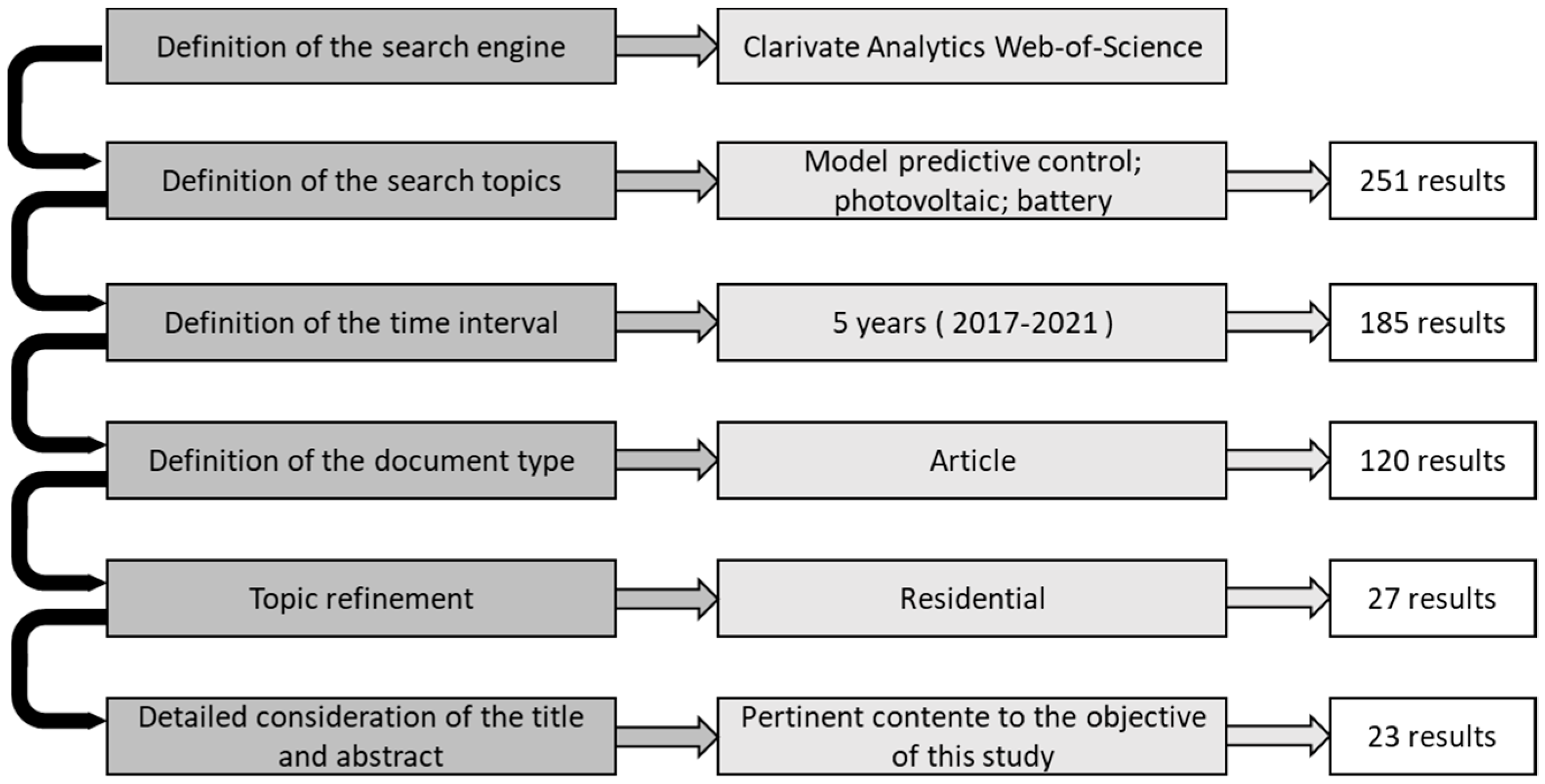
- To provide a review of the most recent works related to the application of MBPC in residential HEMS incorporating photovoltaics and battery systems;
- To provide a sensitivity analysis of MBPC for HEMS, considering the time step, prediction horizon (PH), and control horizon (CH) associated with the data. We show that a significant reduction in the MBPC time complexity with minimal impact on the performance can be obtained by employing a small CH, achieving substantial cost savings, or improved gains, in comparison with many of the approaches found in the literature.
2. State-of-the-Art
2.1. Background Information
2.2. Related Works
3. Methodology
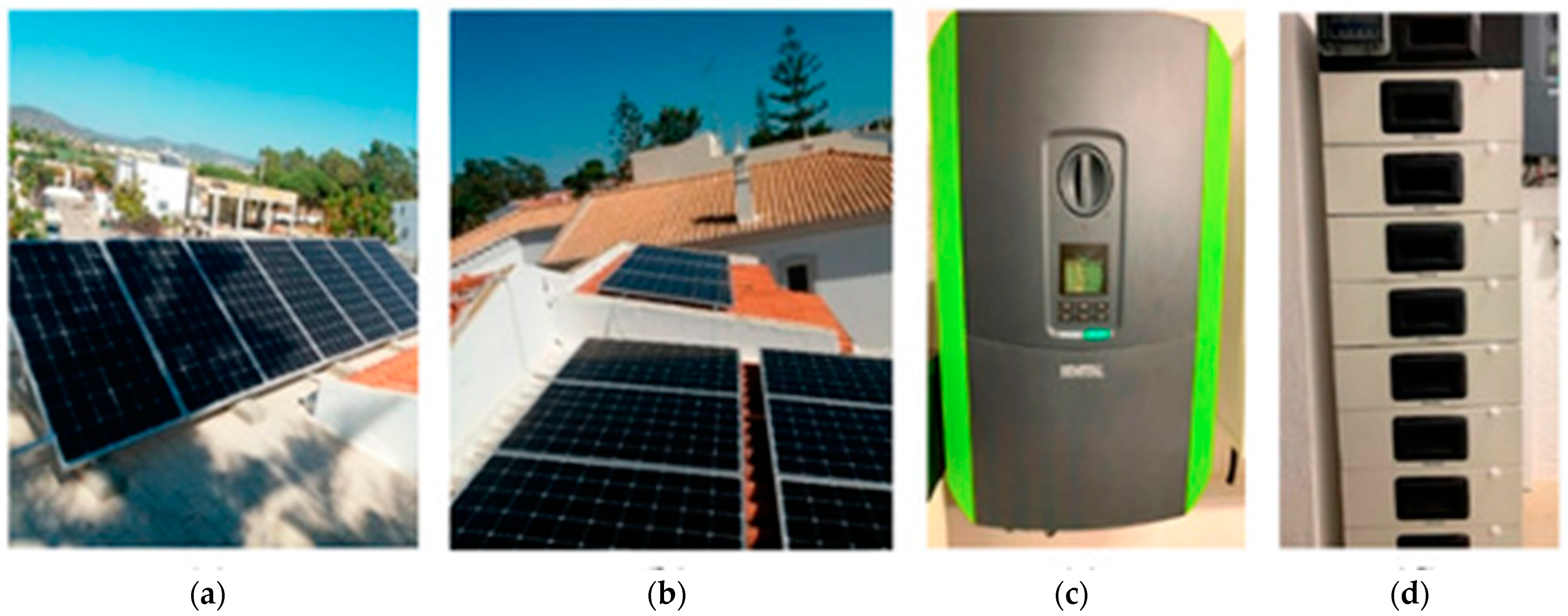
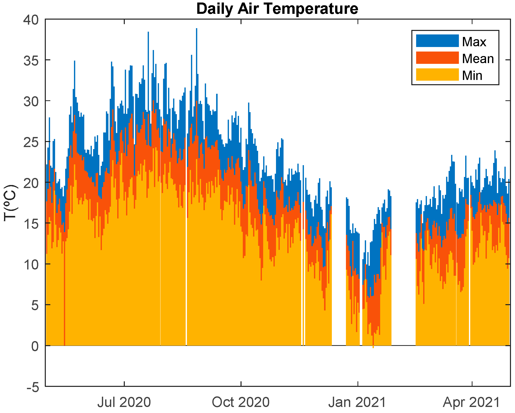
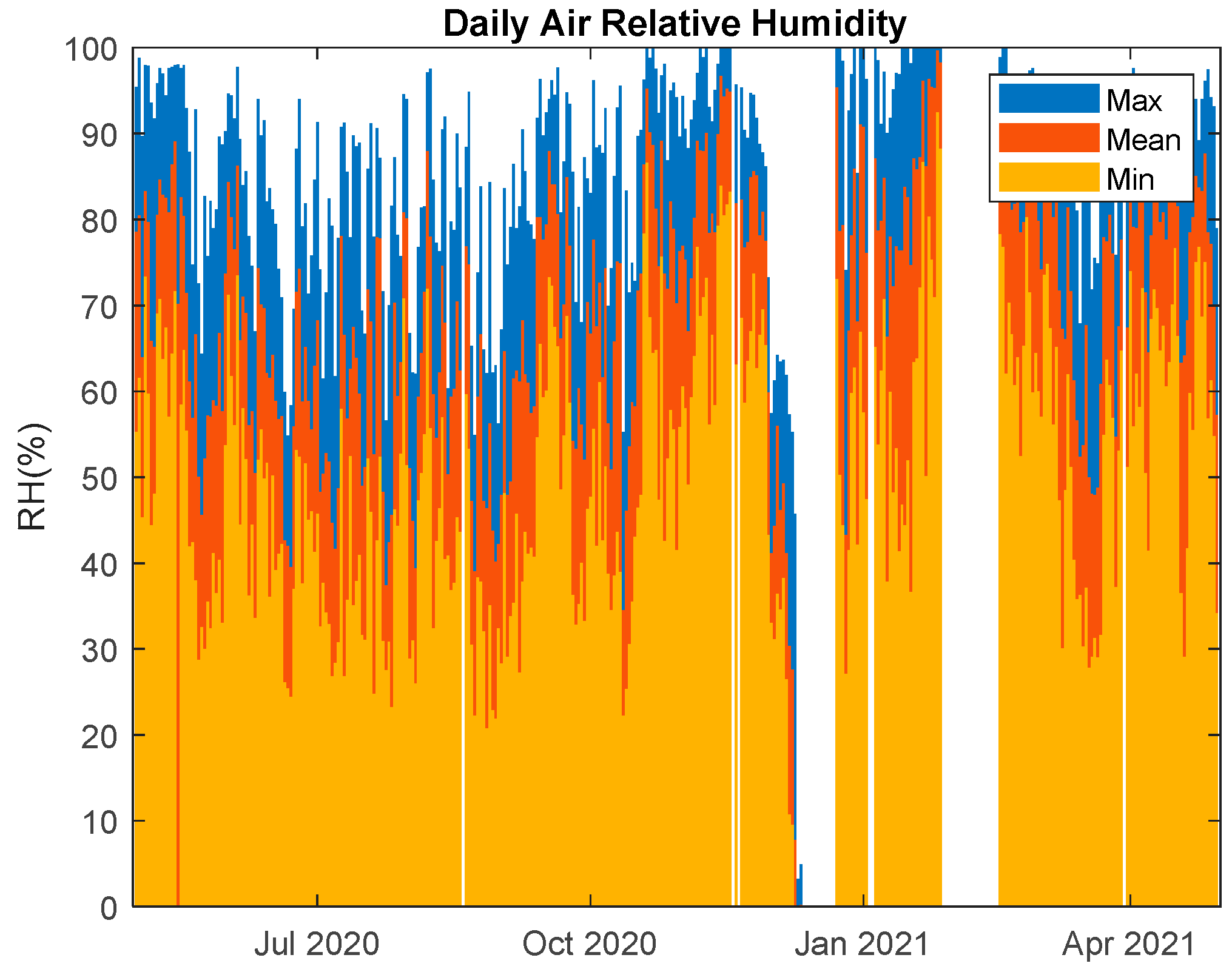
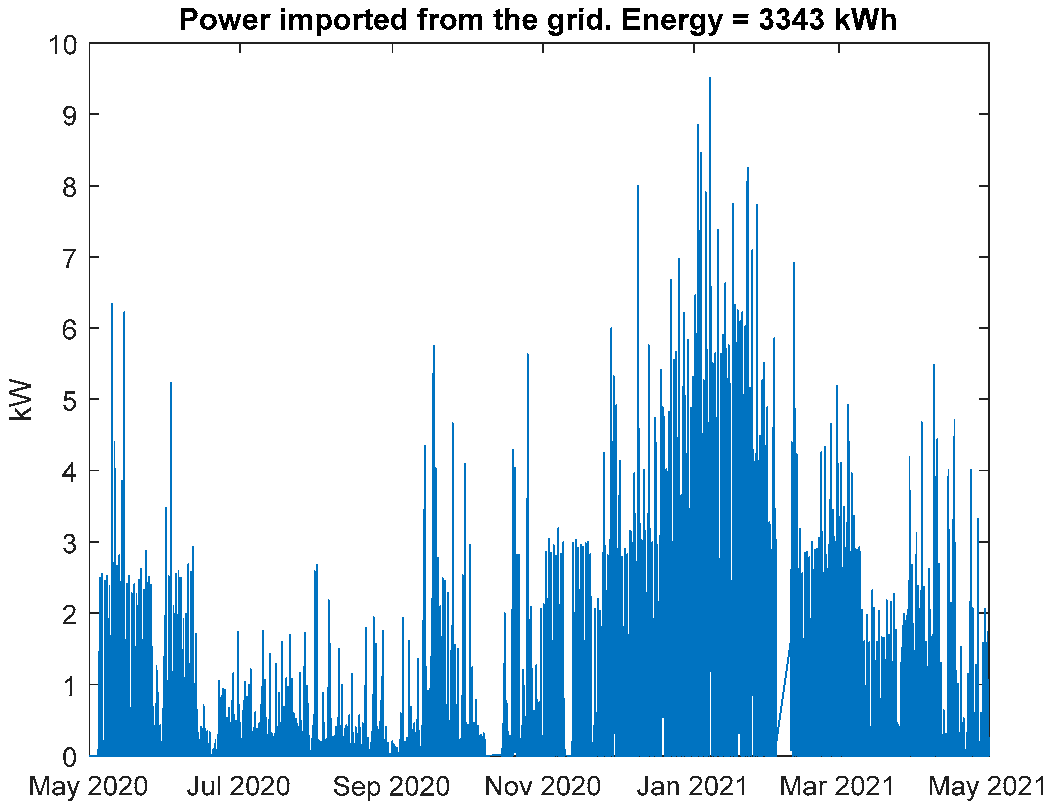
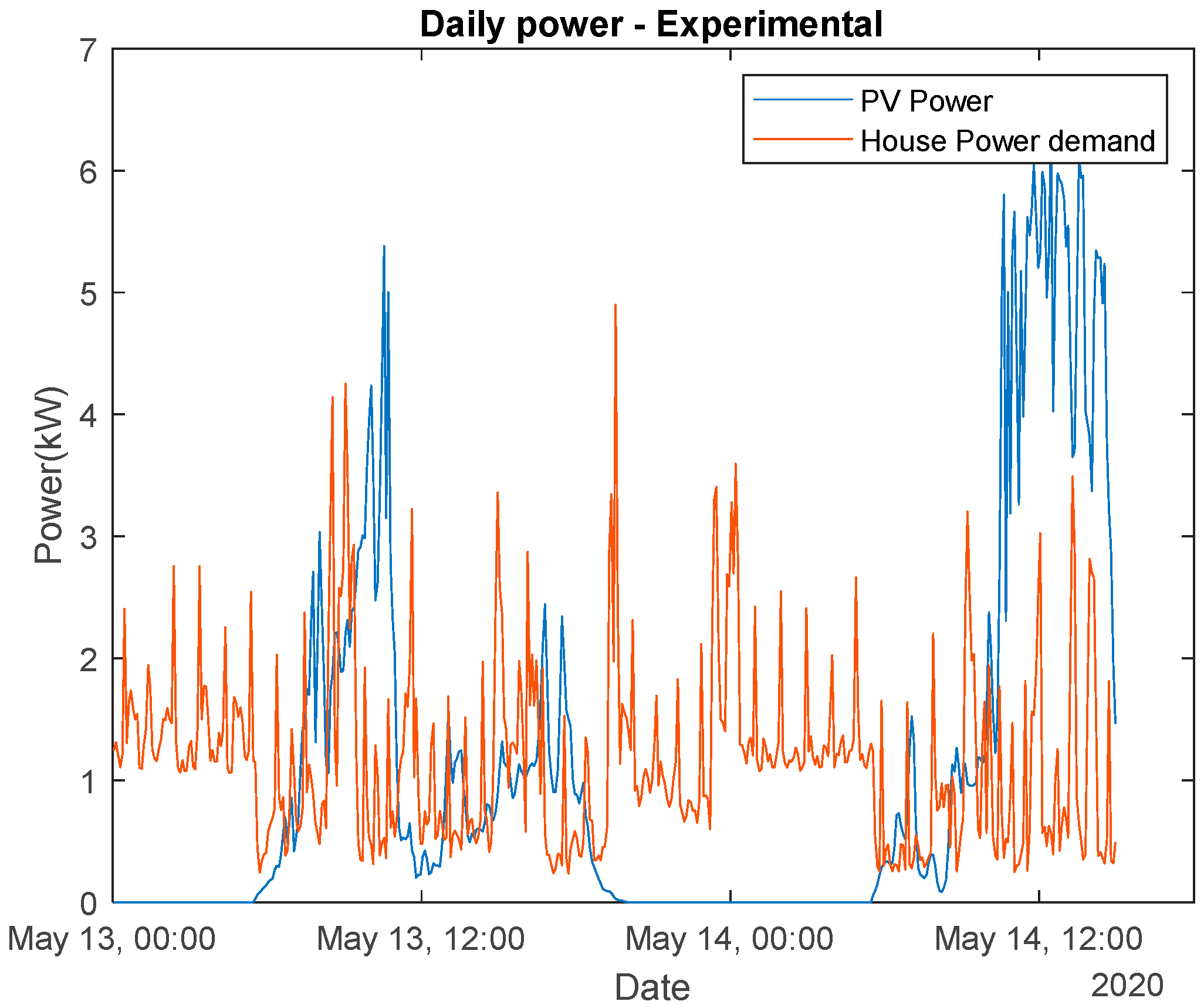
3.1. Case Study
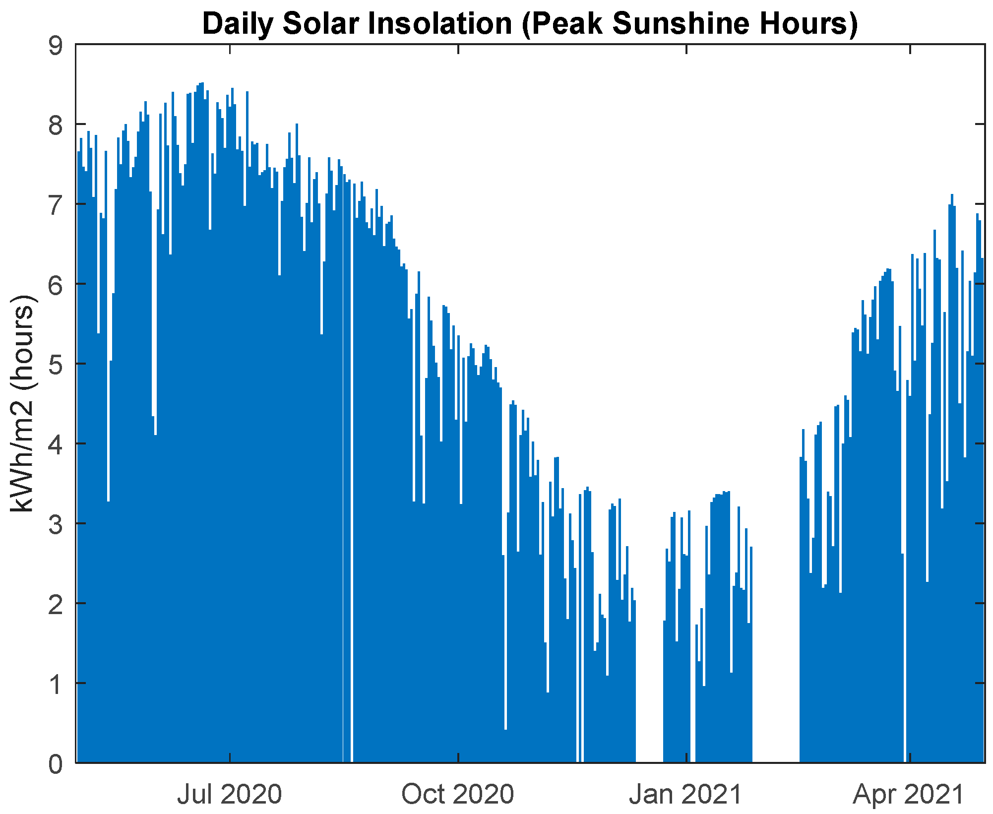
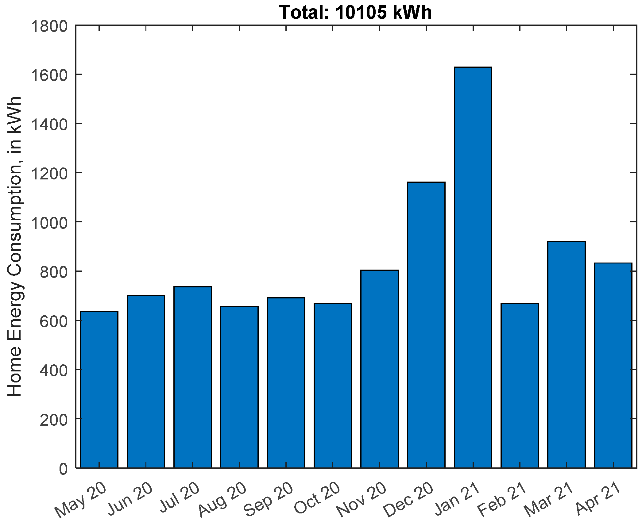
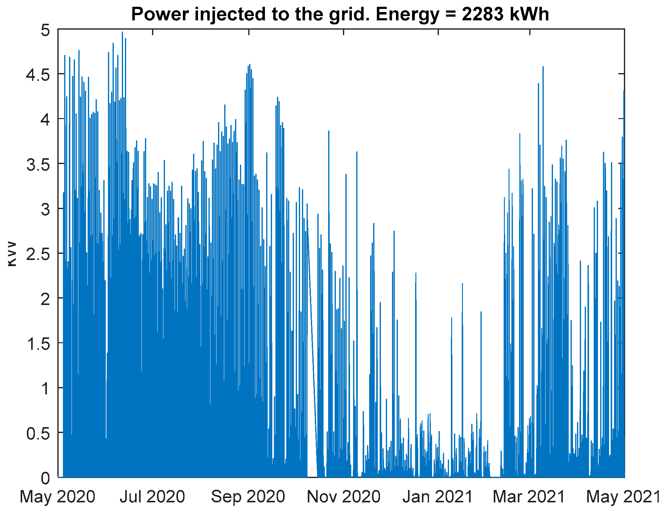
3.2. Household Power Demand and PV Production Profile
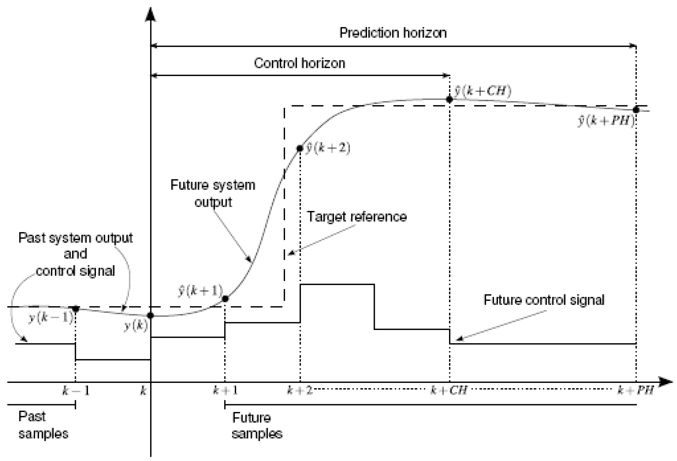
3.3. Formulation of MBPC
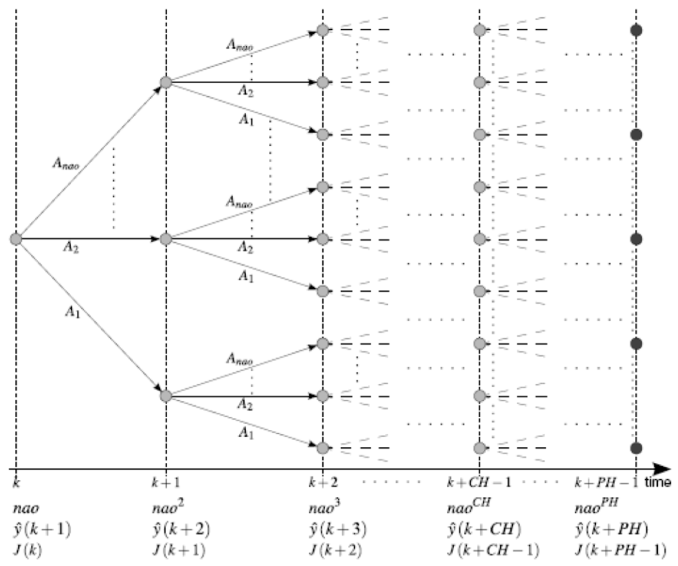
The Branch-and-Bound Algorithm
- an upper bound on the total cost from instant k + 1 to k + PH;
- and a lower bound on the cost from instant k + i to k + PH.
4. Results and Discussion
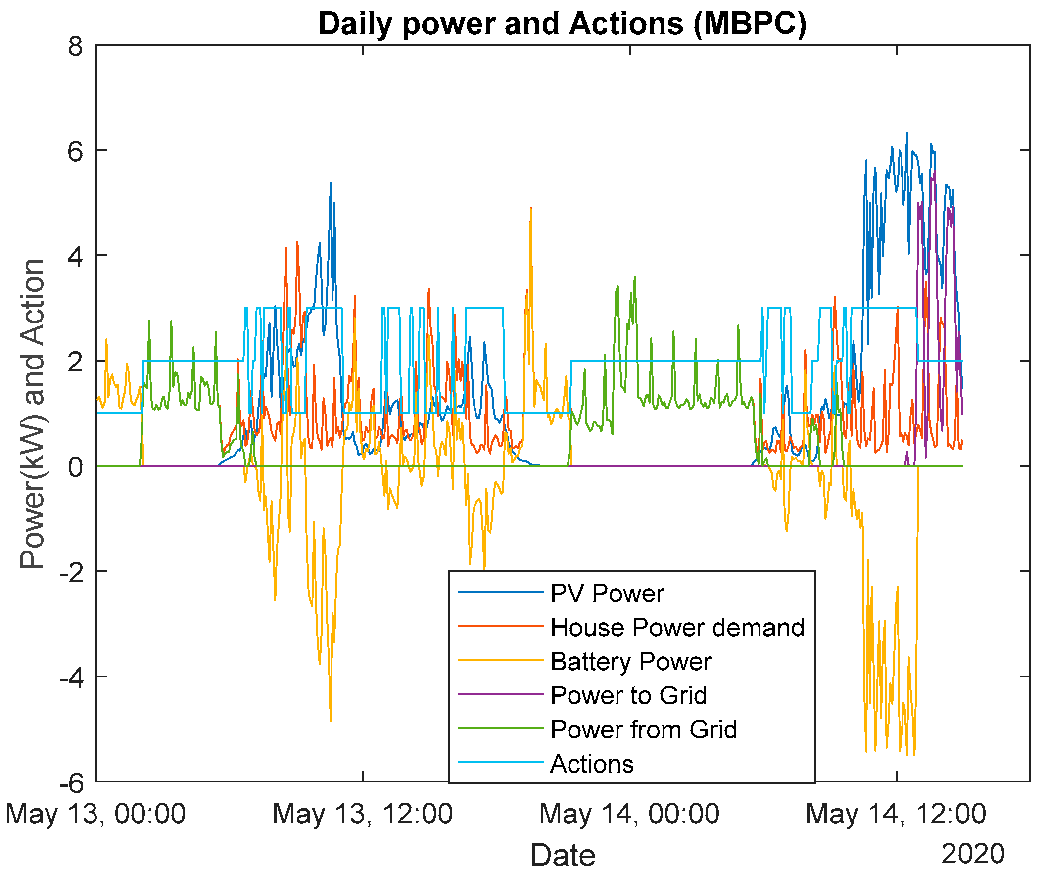
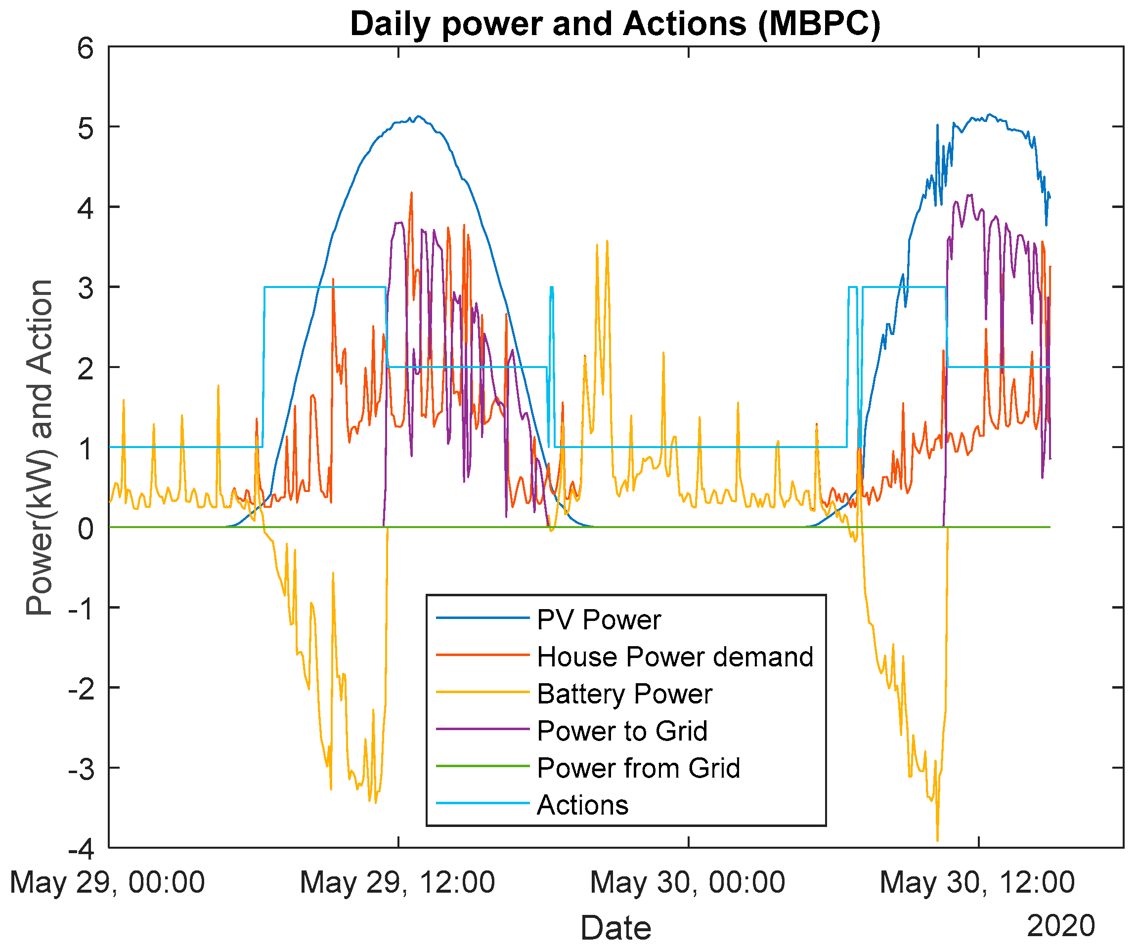
4.1. Model-Based Predictive Control Analysis
4.2. Analysis 1—Prediction Horizon and Time Step Sensitivity Analysis
4.3. Analysis 2—Control Horizon
5. Conclusions
Author Contributions
Funding
Institutional Review Board Statement
Informed Consent Statement
Conflicts of Interest
References
- Zafar, U.; Bayhan, S.; Sanfilippo, A. Home energy management system concepts, configurations, and technologies for the smart grid. IEEE Access 2020, 8, 119271–119286. [Google Scholar] [CrossRef]
- Herczeg, M.; McKinnon, D.; Milos, L.; Bakas, I.; Klaassens, E.; Svatikova, K.; Widerberg, O. Resource Efficiency in the Building Sector; CopenHagen research Institute: Rotterdam, The Netherlands, 2014. [Google Scholar]
- Khan, Z.A.; Ullah, A.; Ullah, W.; Rho, S.; Lee, M.; Baik, S.W. Electrical Energy Prediction in Residential Buildings for Short-Term Horizons Using Hybrid Deep Learning Strategy. Appl. Sci. 2020, 10, 8634. [Google Scholar] [CrossRef]
- Atef, S.; Ismail, N.; Eltawil, A.B. A new fuzzy logic based approach for optimal household appliance scheduling based on electricity price and load consumption prediction. Adv. Build. Energy Res. 2021, 1–19. [Google Scholar] [CrossRef]
- Huang, H.; Xu, H.; Cai, Y.; Khalid, R.S.; Yu, H. Distributed Machine Learning on Smart-Gateway Network toward Real-Time Smart-Grid Energy Management with Behavior Cognition. ACM Trans. Des. Autom. Electron. Syst. 2018, 23, 1–26. [Google Scholar] [CrossRef]
- Mariano-Hernández, D.; Hernández-Callejo, L.; Zorita-Lamadrid, A.; Duque-Pérez, O.; García, F.S. A review of strategies for building energy management system: Model predictive control, demand side management, optimization, and fault detect & diagnosis. J. Build. Eng. 2021, 33, 101692. [Google Scholar]
- Fortenbacher, P.; Ulbig, A.; Andersson, G. Optimal Placement and Sizing of Distributed Battery Storage in Low Voltage Grids Using Receding Horizon Control Strategies. IEEE Trans. Power Syst. 2017, 33, 2383–2394. [Google Scholar] [CrossRef] [Green Version]
- Neves, D.; Silva, C.A. Modeling the impact of integrating solar thermal systems and heat pumps for domestic hot water in electric systems—The case study of Corvo Island. Renew. Energy 2014, 72, 113–124. [Google Scholar] [CrossRef]
- Hossain, M.S.; Mahmood, H. Short-Term Photovoltaic Power Forecasting Using an LSTM Neural Network and Synthetic Weather Forecast. IEEE Access 2020, 8, 172524–172533. [Google Scholar] [CrossRef]
- Kafetzis, A.; Ziogou, C.; Panopoulos, K.; Papadopoulou, S.; Seferlis, P.; Voutetakis, S. Energy management strategies based on hybrid automata for islanded microgrids with renewable sources, batteries and hydrogen. Renew. Sustain. Energy Rev. 2020, 134, 110118. [Google Scholar] [CrossRef]
- Basmadjian, R. Optimized charging of pv-batteries for households using real-time pricing scheme: A model and heuristics-based implementation. Electronics 2020, 9, 113. [Google Scholar] [CrossRef] [Green Version]
- Shakeri, M.; Pasupuleti, J.; Amin, N.; Rokonuzzaman, M.; Low, F.W.; Yaw, C.T.; Asim, N.; Samsudin, N.A.; Tiong, S.K.; Hen, C.K. An overview of the building energy management system considering the demand response programs, smart strategies and smart grid. Energies 2020, 13, 3299. [Google Scholar] [CrossRef]
- Munankarmi, P.; Maguire, J.; Balamurugan, S.P.; Blonsky, M.; Roberts, D.; Jin, X. Community-scale interaction of energy efficiency and demand flexibility in residential buildings. Appl. Energy 2021, 298, 117149. [Google Scholar] [CrossRef]
- Shivam, K.; Tzou, J.C.; Wu, S.C. A multi-objective predictive energy management strategy for residential grid-connected PV-battery hybrid systems based on machine learning technique. Energy Convers. Manag. 2021, 237, 114103. [Google Scholar] [CrossRef]
- Van der Meer, D.; Wang, G.C.; Munkhammar, J. An alternative optimal strategy for stochastic model predictive control of a residential battery energy management system with solar photovoltaic. Appl. Energy 2021, 283, 116289. [Google Scholar] [CrossRef]
- Su, H.; Zhou, Y.; Feng, D.H.; Li, H.J.; Numan, M. Optimal energy management of residential battery storage under uncertainty. Int. Trans. Electr. Energy Syst. 2021, 31, e12713. [Google Scholar] [CrossRef]
- Mbungu, N.T.; Bansal, R.C.; Naidoo, R.M.; Bettayeb, M.; Siti, M.W.; Bipath, M. A dynamic energy management system using smart metering. Appl. Energy 2020, 280, 115990. [Google Scholar] [CrossRef]
- Langer, L.; Volling, T. An optimal home energy management system for modulating heat pumps and photovoltaic systems. Appl. Energy 2020, 278, 115661. [Google Scholar] [CrossRef]
- Narayanan, M.; de Lima, A.F.; Dantas, A.; Commerell, W. Development of a Coupled TRNSYS-MATLAB Simulation Framework for Model Predictive Control of Integrated Electrical and Thermal Residential Renewable Energy System. Energies 2020, 13, 5761. [Google Scholar] [CrossRef]
- Banfield, B.; Robinson, D.A.; Agalgaonkar, A.P. Comparison of economic model predictive control and rule-based control for residential energy storage systems. IET Smart Grid 2020, 3, 722–729. [Google Scholar] [CrossRef]
- Mbuwir, B.V.; Geysen, D.; Spiessens, F.; Deconinck, G. Reinforcement learning for control of flexibility providers in a residential microgrid. IET Smart Grid 2020, 3, 98–107. [Google Scholar] [CrossRef]
- Kersic, M.; Bocklisch, T.; Bottiger, M.; Gerlach, L. Coordination Mechanism for PV Battery Systems with Local Optimizing Energy Management. Energies 2020, 13, 611. [Google Scholar] [CrossRef] [Green Version]
- Yousefi, M.; Hajizadeh, A.; Soltani, M.N.; Hredzak, B. Predictive Home Energy Management System With Photovoltaic Array, Heat Pump, and Plug-In Electric Vehicle. IEEE Trans. Ind. Inform. 2021, 17, 430–440. [Google Scholar] [CrossRef]
- Galvan, E.; Mandal, P.; Chakraborty, S.; Senjyu, T. Efficient Energy-Management System Using A Hybrid Transactive-Model Predictive Control Mechanism for Prosumer-Centric Networked Microgrids. Sustainability 2019, 11, 5436. [Google Scholar] [CrossRef] [Green Version]
- Kuboth, S.; Heberle, F.; König-Haagen, A.; Brüggemann, D. Economic model predictive control of combined thermal and electric residential building energy systems. Appl. Energy 2019, 240, 372–385. [Google Scholar] [CrossRef]
- Wang, R.G.; Zhang, X.N.; Bao, J. A self-interested distributed economic model predictive control approach to battery energy storage networks. J. Process. Control 2019, 73, 9–18. [Google Scholar] [CrossRef]
- Alramlawi, M.; Gabash, A.; Mohagheghi, E.; Li, P. Optimal operation of hybrid PV-battery system considering grid scheduled blackouts and battery lifetime. Sol. Energy 2018, 161, 125–137. [Google Scholar] [CrossRef]
- Kneiske, T.M.; Braun, M.; Hidalgo-Rodriguez, D.I. A new combined control algorithm for PV-CHP hybrid systems. Appl. Energy 2018, 210, 964–973. [Google Scholar] [CrossRef]
- Khalid, M.; Akram, U.; Shafiq, S. Optimal Planning of Multiple Distributed Generating Units and Storage in Active Distribution Networks. IEEE Access 2018, 6, 55234–55244. [Google Scholar] [CrossRef]
- Zhang, X.N.; Bao, J.; Wang, R.G.; Zheng, C.X.; Skyllas-Kazacos, M. Dissipativity based distributed economic model predictive control for residential microgrids with renewable energy generation and battery energy storage. Renew. Energy 2017, 100, 18–34. [Google Scholar] [CrossRef]
- Baniasadi, A.; Habibi, D.; Al-Saedi, W.; Masoum, M.A.S.; Das, C.K.; Mousavi, N. Optimal sizing design and operation of electrical and thermal energy storage systems in smart buildings. J. Energy Storage 2020, 28, 101186. [Google Scholar] [CrossRef]
- Seal, S.; Boulet, B.; Dehkordi, V.R. Centralized model predictive control strategy for thermal comfort and residential energy management. Energy 2020, 212, 118456. [Google Scholar] [CrossRef]
- Jin, X.; Baker, K.; Christensen, D.; Isley, S. Foresee: A user-centric home energy management system for energy efficiency and demand response. Appl. Energy 2017, 205, 1583–1595. [Google Scholar] [CrossRef]
- Kuboth, S.; Heberle, F.; Weith, T.; Welzl, M.; Konig-Haagen, A.; Bruggemann, D. Experimental short-term investigation of model predictive heat pump control in residential buildings. Energy Build. 2019, 204, 109444. [Google Scholar] [CrossRef]
- Ruano, A.; Silva, S.; Duarte, H.; Ferreira, P.M. Wireless Sensors and IoT Platform for Intelligent HVAC Control. Appl. Sci. 2018, 8, 370. [Google Scholar] [CrossRef] [Green Version]
- Ruano, A.; Bot, K.; Ruano, M.G. Home Energy Management System in an Algarve residence. First results. In CONTROLO 2020: Proceedings of the 14th APCA International Conference on Automatic Control and Soft Computing; Gonçalves, J.A., Braz-César, M., Coelho, J.P., Eds.; Lecture Notes in Electrical Engineering 695; Springer Science and Business Media Deutschland GmbH: Bragança, Portugal, 2021; pp. 332–341. [Google Scholar]
- Ruano, A.; Bot, K.; Ruano, M.d.G. The Impact of Occupants in Thermal Comfort and Energy Efficiency in Buildings. In Occupant Behaviour in Buildings: Advances and Challenges; Bentham Science: Sharjah, United Arab Emirates, 2021; Volume 6, pp. 101–137. [Google Scholar]
- Mestre, G.; Ruano, A.; Duarte, H.; Silva, S.; Khosravani, H.; Pesteh, S.; Ferreira, P.; Horta, R. An Intelligent Weather Station. Sensors 2015, 15, 31005–31022. [Google Scholar] [CrossRef]
- Bot, K.; Ruano, A.; Ruano, M.d.G. Short-Term Forecasting Photovoltaic Solar Power for Home Energy Management Systems. Inventions 2021, 6, 12. [Google Scholar] [CrossRef]
- Clarke, D.W.; Mohtadi, C.; Tuffs, P.S. Generalized predictive control—Part I. the basic algorithm. Automatica 1987, 23, 137–148. [Google Scholar] [CrossRef]
- Ferreira, P.M. Application of Computational Intelligence Methods to Greenhouse Environmental Control. Ph.D. Thesis, Algarve University, Faro, Portugal, 2007. [Google Scholar]
- Sousa, J.M.; Babuška, R.; Verbruggen, H.B. Fuzzy predictive control applied to an air-conditioning system. Control. Eng. Pract. 1997, 5, 1395–1406. [Google Scholar] [CrossRef]
- Ferreira, P.M.; Silva, S.M.; Ruano, A.E. Model based predictive control of HVAC systems for human thermal comfort and energy consumption minimisation. IFAC Proc. Vol. 2012, 45, 236–241. [Google Scholar] [CrossRef]
- Ruano, A.E.; Pesteh, S.; Silva, S.; Duarte, H.; Mestre, G.; Ferreira, P.M.; Khosravani, H.R.; Horta, R. The IMBPC HVAC system: A complete MBPC solution for existing HVAC systems. Energy Build. 2016, 120, 145–158. [Google Scholar] [CrossRef]
- Tian, W. A review of sensitivity analysis methods in building energy analysis. Renew. Sustain. Energy Rev. 2013, 20, 411–419. [Google Scholar] [CrossRef]
- Christopher Frey, H.; Patil, S.R. Identification and review of sensitivity analysis methods. Risk Anal. 2002, 22, 553–578. [Google Scholar] [CrossRef]
- Parisio, A.; Rikos, E.; Glielmo, L. A Model Predictive Control Approach to Microgrid Operation Optimization. IEEE Trans. Control Syst. Technol. 2014, 22, 1813–1827. [Google Scholar] [CrossRef]
- D’Ettorre, F.; Conti, P.; Schito, E.; Testi, D. Model predictive control of a hybrid heat pump system and impact of the prediction horizon on cost-saving potential and optimal storage capacity. Appl. Therm. Eng. 2018, 148, 524–535. [Google Scholar] [CrossRef]
- Bot, K.; Ruano, A.; Ruano, M. Forecasting Electricity Demand in Households using MOGA-designed Artificial Neural Networks. IFAC-PapersOnLine 2020, 53, 8225–8230. [Google Scholar] [CrossRef]
- Bot, K.; Ruano, A.; Ruano, M.d.G. Forecasting Electricity Consumption in Residential Buildings for Home Energy Management Systems. In Information Processing and Management of Uncertainty in Knowledge-Based Systems (IPMU); Lesot, M.-J., Vieira, S., Reformat, M.Z., Carvalho, J.P., Wilbik, A., Bouchon-Meunier, B., Yager, R.R., Eds.; Springer International Publishing: Berlin/Heidelberg, Germany, 2020; Volume 1237, pp. 313–326. [Google Scholar]


| Technique | Description |
|---|---|
| Linear Programming (LP) | Models’ relationship between variables as linear to maximize or minimize an objective. |
| MILP | Similar to LP; however, additional constraints are put on at least one decision variable so that they have to be discrete. |
| Convex Programming | Minimizes a convex or maximizes a concave objective function. |
| Genetic Programming | A heuristic search method inspired by biology and iteratively produces “fitter” candidates using “crossover” and “mutation” functions. |
| Particle Swarm Optimization | A heuristic search that iteratively produces better candidates using “position”, “velocity”, and “fitness” values |
| Model Predictive Control | Uses a model to predict plant/required output. It chooses a “control action” by repeatedly solving an online optimization problem. |
| Game Theory | Models the iteration between different “players” and the environment using fixed rules. |
| Artificial Neural Networks (ANN) | A modelling techniques using artificial neurons to create complex models for forecasting and classification. |
| Fuzzy Logic Control (FLC) | Uses a rule-based system to produce an output for forecasting or classification. |
| Reinforcement Learning | A machine learning methodology that learns how to maximize a reward function through trial and error. |
| Scenario Nº | Start Day | End Day | Time Step (min) | Prediction Horizon | Control Horizon | Comp Time (s) |
|---|---|---|---|---|---|---|
| Cloudy Day | ||||||
| S1 | 13 May 2020 | 14 May 2020 | 5 | 12 | 12 | 0.61 |
| S2 | 13 May 2020 | 14 May 2020 | 10 | 12 | 12 | 0.35 |
| S3 | 13 May 2020 | 14 May 2020 | 15 | 12 | 12 | 0.14 |
| S4 | 13 May 2020 | 14 May 2020 | 5 | 24 | 24 | 188.86 |
| S5 | 13 May 2020 | 14 May 2020 | 10 | 24 | 24 | 9.95 |
| S6 | 13 May 2020 | 14 May 2020 | 15 | 24 | 24 | 18.52 |
| S7 | 13 May 2020 | 14 May 2020 | 5 | 36 | 36 | 4987.00 |
| S8 | 13 May 2020 | 14 May 2020 | 10 | 36 | 36 | 5.51 |
| S9 | 13 May 2020 | 14 May 2020 | 15 | 36 | 36 | 312.00 |
| Sunny Day | ||||||
| S10 | 29 May 2020 | 30 May 2020 | 5 | 12 | 12 | 0.77 |
| S11 | 29 May 2020 | 30 May 2020 | 10 | 12 | 12 | 0.27 |
| S12 | 29 May 2020 | 30 May 2020 | 15 | 12 | 12 | 0.12 |
| S13 | 29 May 2020 | 30 May 2020 | 5 | 24 | 24 | 0.98 |
| S14 | 29 May 2020 | 30 May 2020 | 10 | 24 | 24 | 0.47 |
| S15 | 29 May 2020 | 30 May 2020 | 15 | 24 | 24 | 0.35 |
| S16 | 29 May 2020 | 30 May 2020 | 5 | 36 | 36 | 1.95 |
| S17 | 29 May 2020 | 30 May 2020 | 10 | 36 | 36 | 0.86 |
| S18 | 29 May 2020 | 30 May 2020 | 15 | 36 | 36 | 0.61 |
| Scenario Nº | Start Day | End Day | Step Time (min) | Prediction Horizon | Control Horizon | Comp Time (s) |
|---|---|---|---|---|---|---|
| Cloudy Day | ||||||
| A1 | 13 May 2020 | 14 May 2020 | 5 | 36 | 2 | 0.05 |
| A2 | 13 May 2020 | 14 May 2020 | 5 | 36 | 3 | 0.18 |
| A3 | 13 May 2020 | 14 May 2020 | 5 | 36 | 4 | 0.25 |
| A4 | 13 May 2020 | 14 May 2020 | 15 | 36 | 2 | 0.18 |
| A5 | 13 May 2020 | 14 May 2020 | 15 | 36 | 3 | 0.11 |
| A6 | 13 May 2020 | 14 May 2020 | 15 | 36 | 4 | 0.05 |
| Sunny Day | ||||||
| A7 | 29 May 2020 | 30 May 2020 | 5 | 36 | 2 | 0.15 |
| A8 | 29 May 2020 | 30 May 2020 | 5 | 36 | 3 | 0.21 |
| A9 | 29 May 2020 | 30 May 2020 | 5 | 36 | 4 | 0.20 |
| A10 | 29 May 2020 | 30 May 2020 | 15 | 36 | 2 | 0.33 |
| A11 | 29 May 2020 | 30 May 2020 | 15 | 36 | 3 | 0.12 |
| A12 | 29 May 2020 | 30 May 2020 | 15 | 36 | 4 | 0.09 |
Publisher’s Note: MDPI stays neutral with regard to jurisdictional claims in published maps and institutional affiliations. |
© 2021 by the authors. Licensee MDPI, Basel, Switzerland. This article is an open access article distributed under the terms and conditions of the Creative Commons Attribution (CC BY) license (https://creativecommons.org/licenses/by/4.0/).
Share and Cite
Bot, K.; Laouali, I.; Ruano, A.; Ruano, M.d.G. Home Energy Management Systems with Branch-and-Bound Model-Based Predictive Control Techniques. Energies 2021, 14, 5852. https://doi.org/10.3390/en14185852
Bot K, Laouali I, Ruano A, Ruano MdG. Home Energy Management Systems with Branch-and-Bound Model-Based Predictive Control Techniques. Energies. 2021; 14(18):5852. https://doi.org/10.3390/en14185852
Chicago/Turabian StyleBot, Karol, Inoussa Laouali, António Ruano, and Maria da Graça Ruano. 2021. "Home Energy Management Systems with Branch-and-Bound Model-Based Predictive Control Techniques" Energies 14, no. 18: 5852. https://doi.org/10.3390/en14185852
APA StyleBot, K., Laouali, I., Ruano, A., & Ruano, M. d. G. (2021). Home Energy Management Systems with Branch-and-Bound Model-Based Predictive Control Techniques. Energies, 14(18), 5852. https://doi.org/10.3390/en14185852