Dynamic Voltage Stability Assessment in Remote Island Power System with Renewable Energy Resources and Virtual Synchronous Generator

Abstract

Increasing the proportion of renewable energy generations in remote island power systems is becoming essential for realizing decarbonized society. However, since inverter-connected renewable energies have different generation characteristics from conventional generators, the massive penetration can adversely affect system stability. In particular, fault events in such weak remote systems can cause fast voltage collapse, and there is a need to assess dynamic voltage stability. This study attempts dynamic voltage stability assessment using the critical boundary index (CBI) and investigates the impact of the virtual synchronous generator (VSG) on dynamic voltage stability. A remote island power system and VSG are modeled, and time-domain simulations are conducted with case studies of fault events. The simulation results show the potential of CBI to use for dynamic voltage stability assessment. Furthermore, the VSG can provide suitable power output during fault events and improve dynamic voltage stability.

1. Introduction

The rapid spread of the sustainable development goals (SDGs) over the past few years has increased the pressure to reduce carbon emissions, and the introduction of renewable energies for energy decarbonization is becoming increasingly important. However, inverter-connected renewable energies have different generation characteristics from conventional generators, which adversely affect system stability. Consequently, weak remote island power systems tend to be highly dependent on thermal power generation, and increasing the proportion of renewable energy generation is one of the most challenging issues.

Various researches have investigated the impact of renewable energies on system stability. The impact of the momentary cessation mode of inverter-connected distributed power supply on transient stability has been described [1]. A Moroccan case study suggests that large-scale integration of renewable energies reduces system inertia and reduces dynamic stability against sudden load and power generation changes [2]. In order to treat the uncertainty of renewable energies, a probabilistic two-stage voltage stability assessment has been proposed [3]. Transient stability probability assessment in high penetration renewable energy grids has been studied to achieve dynamic reactive power configuration [4]. The effect of various configurations of hybrid renewable energy source plants on system stability has been verified [5].

Virtual synchronous generator (VSG) technology is gaining attention to solve the instability posed by renewable energies. Since VSG can provide simulated inertia as a synchronous generator, they are expected to improve system stability. A few works have studied the impact of VSG on stability. In [6], the authors have investigated the impact of VSG integration on transient stability and observed that a modified VSG improves transient stability. The application of a VSG with variable inertia has been proposed to address the transient instability caused by PV penetration [7]. A new VSG frequency control method to improve the frequency stability of an islanded microgrid has been developed in [8].

Despite many studies, the investigation of voltage stability is insufficient. Some of the studies have addressed static voltage stability assessment [3,4,5]. However, since fault events in weak remote systems can cause fast voltage collapse, there is a need to assess the dynamic variation of voltage stability. The transient voltage stability index (TVSI) proposed in [9], based on the magnitude and duration of voltage fluctuations, is often used for short-term voltage stability assessment. However, it is not suitable for quantifying proximity to voltage collapse during disturbances. Moreover, few studies have investigated the impact of VSG on voltage stability.

Many studies have proposed voltage stability indices to quantify proximity to voltage collapse [10,11,12,13,14]. Most of them represent the proximity to voltage collapse by a value normalized between 0 and 1. In contrast, a critical boundary index (CBI) based on active and reactive power deviations ($\Delta P$ and $\Delta Q$) has been proposed in [15]. CBI represents the proximity to voltage collapse by par unit (pu), and the values of $\Delta P$ and $\Delta Q$ can evaluate the margin of active and reactive power to the unstable region. The authors in [15] have summarized the literature [10,11,12,13,14] and conducted a detailed comparative study. The results show that CBI performs better than the existing indices. However, the studied voltage stability indices only consider static voltage stability assessment.

On the other hand, authors in [16] have proposed the P-index normalized between 0 and 1 and applied it to online monitoring. However, severe dynamic cases where the voltage stability decreases rapidly have not been considered. We are interested in whether the advantages of CBI can be utilized in such dynamic situations. Since the $\Delta P$ and $\Delta Q$ values in dynamic situations may be available for proper control of VSG, it is worth investigating the availability of CBI and the impact of VSG.

This study attempts to apply CBI to assess dynamic voltage stability and investigates the impact of VSG on voltage stability. Section 2 introduces the concept and calculation of CBI. Section 3 describes a VSG model and control strategy. Section 4 presents the simulation results for case studies and discusses the proposed dynamic voltage stability assessment and the impact of VSG. Finally, Section 5 concludes this paper.

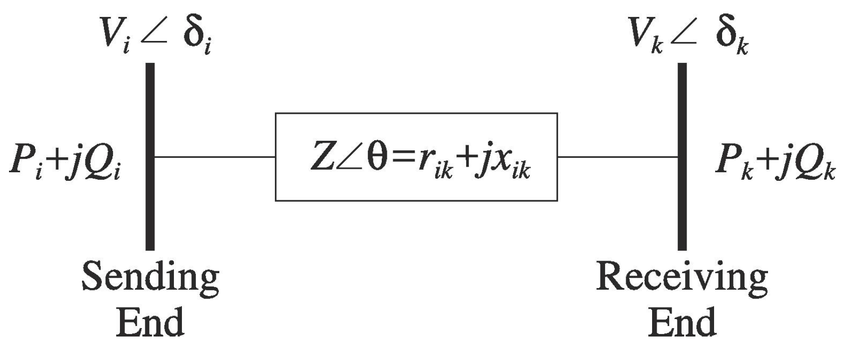
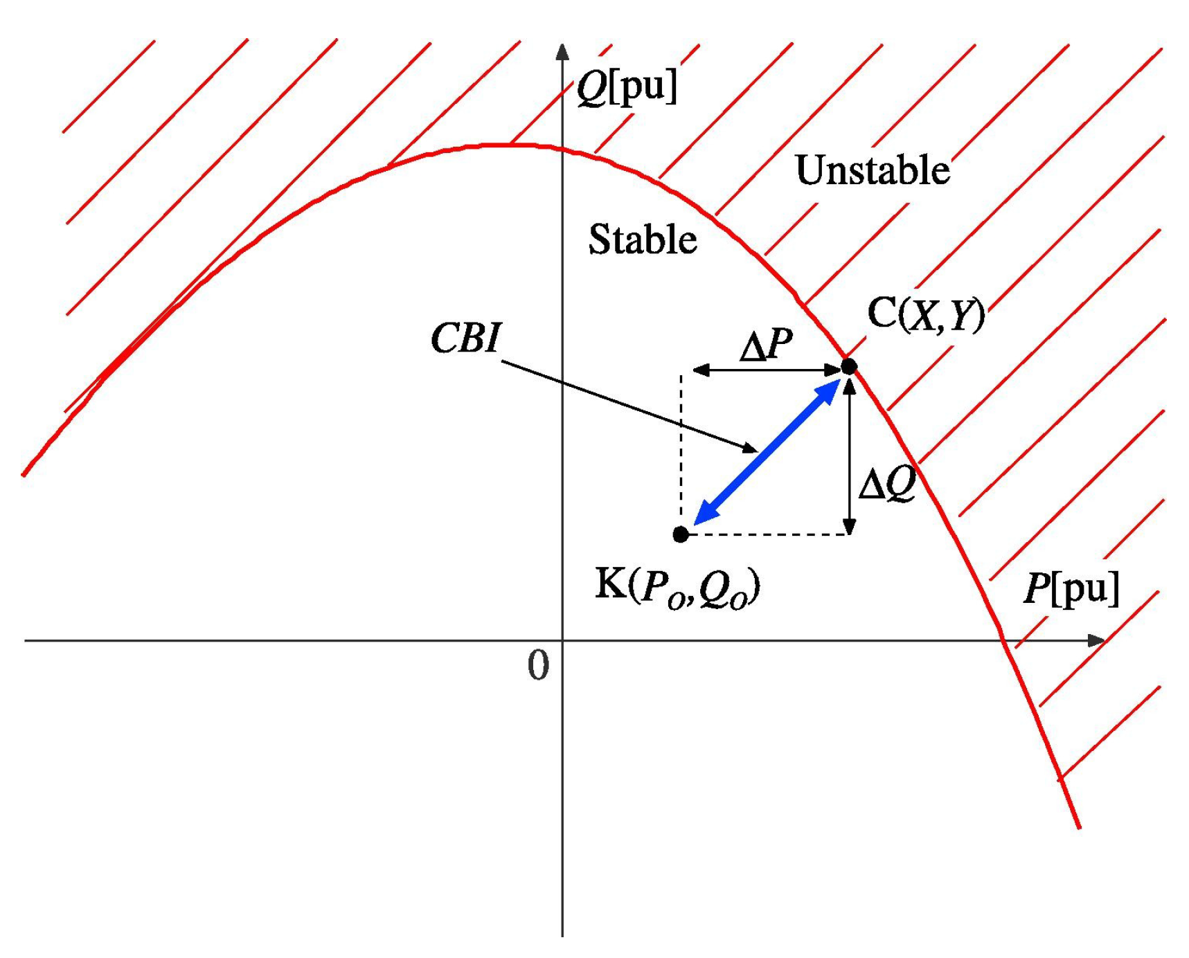
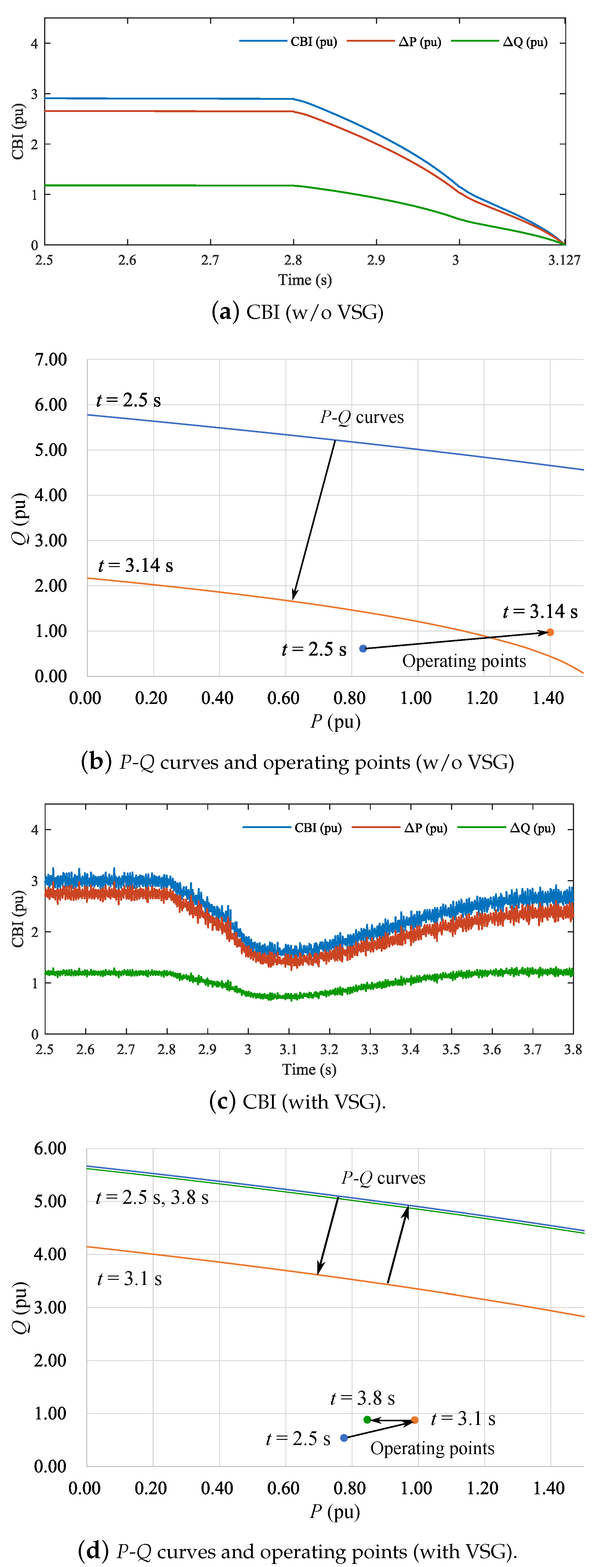
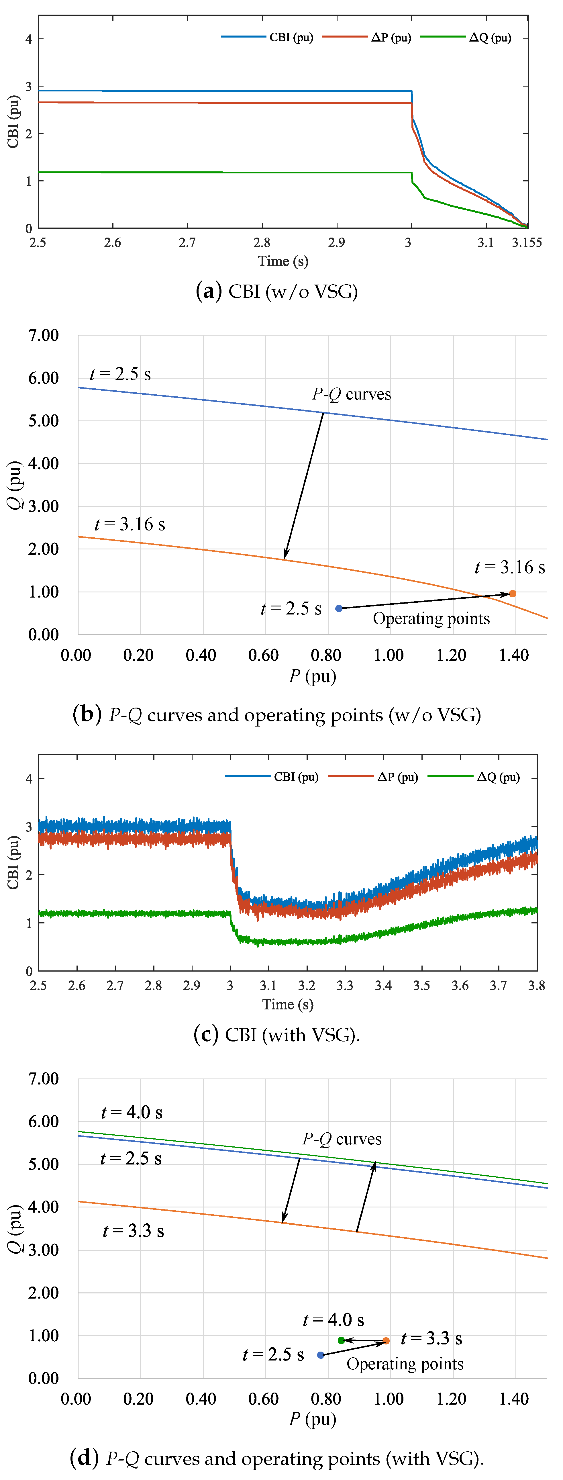
2. Critical Boundary Index (CBI)

The CBI is first proposed in [15]. It can be derived from the power flow equation of the 2-bus transmission line shown in Figure 1. The power flow equation is given by

$$\begin{array}{c}\hfill P_k+j{Q}_k=(V_k\angle {\delta }_k){\left(\frac{V_i\angle {\delta }_i-V_k\angle {\delta }_k}{r_{ik}+j{x}_{ik}}\right)}^{*},\end{array}$$

(1)

where, $V_i\angle {\delta }_i$ and $V_k\angle {\delta }_k$ are the sending and receiving end voltage phasers, respectively; $P_k$ and $Q_k$ are the active and reactive power received at the receiving end, respectively; $P_i$ and $Q_i$ are the active and reactive power sent from the sending end, respectively; and $r_{ik}$ and $x_{ik}$ are the line resistance and reactance, respectively. Transforming (1) and solving for $V_k$, the following equation can be obtained [15]:

$$\begin{array}{cc}\hfill & V_k=\sqrt{-\left(r_{ik}{P}_k+x_{ik}{Q}_k-\frac{V_i^2}{2}\right)\pm A},\hfill \end{array}$$

(2)

$$\begin{array}{cc}\hfill & A=\sqrt{{\left(r_{ik}{P}_k+x_{ik}{Q}_k-\frac{V_i^2}{2}\right)}^2-(r_{ik}^2+x_{ik}^2)(P_k^2+Q_k^2)}.\hfill \end{array}$$

(3)

From (2) and (3), the operating point at which $A=0$ indicates the voltage collapse point. Here, solving $A=0$ for $Q_k$, we can derive [15]

$$\begin{array}{c}\hfill Q_k=\frac{\pm \sqrt{x_{ik}^2{V}_i^4+r_{ik}^2{V}_i^4-4x_{ik}^2{r}_{ik}{V}_i^2{P}_k-4r_{ik}^3{V}_i^2{P}_k}}{2r_{ik}^2}+\frac{2x_{ik}{r}_{ik}{P}_k-x_{ik}{V}_i^2}{2r_{ik}^2}.\end{array}$$

(4)

From (4), the P-Q characteristics can be visualized as Figure 2.

In Figure 2, the red P-Q curve shows the boundary between stable and unstable regions. The value of CBI means the minimum distance between the current operating point $K(P_o,Q_o)$ and critical boundary point $C(X,Y)$ on the P-Q curve.

In order to calculate CBI, the Lagrange multiplier is applied. First, (3) can be rewritten as [15]

$$\begin{array}{c}\hfill C(X,Y)={\left(r_{ik}X+x_{ik}Y-\frac{V_i^2}{2}\right)}^2-(r_{ik}^2+x_{ik}^2)(X^2+Y^2)=0.\end{array}$$

(5)

Then the distance between $K(P_o,Q_o)$ and $C(X,Y)$ can be expressed by the function $f(X,Y)$. It is given by [15]

$$\begin{array}{c}\hfill f^2={(X-P_o)}^2+{(Y-Q_o)}^2.\end{array}$$

(6)

Using the Lagrange multiplier, the following equation is obtained [15]:

$$\begin{array}{lll}F(X,Y,\lambda )& =& f^2(X,Y)-\lambda C(X,Y)\hfill \\ & =& {(X-P_o)}^2+{(Y-Q_o)}^2\hfill \\ & & -\lambda \left({\left(r_{ik}X+x_{ik}Y-\frac{V_i^2}{2}\right)}^2-(r_{ik}^2+x_{ik}^2)(X^2+Y^2)\right).\hfill \end{array}$$

(7)

Partial differentiation of (7) with respect to X, Y, and $\lambda$ yields the following equations [15]:

$$\begin{array}{cc}\hfill & 2X-2P_o-\lambda \left(2\left(r_{ik}X+x_{ik}Y-\frac{V_i^2}{2}\right)r_{ik}-2(r_{ik}^2+x_{ik}^2)X\right)=0,\hfill \end{array}$$

(8)

$$\begin{array}{cc}\hfill & 2Y-2Q_o-\lambda \left(2\left(r_{ik}X+x_{ik}Y-\frac{V_i^2}{2}\right)x_{ik}-2(r_{ik}^2+x_{ik}^2)Y\right)=0,\hfill \end{array}$$

(9)

$$\begin{array}{cc}\hfill & -{\left(r_{ik}X+x_{ik}Y-\frac{V_i^2}{2}\right)}^2+(r_{ik}^2+x_{ik}^2)(X^2+Y^2)=0.\hfill \end{array}$$

(10)

By solving the simultaneous equations consisting of (8)–(10), the value of X, Y and $\lambda$ are obtained. In other words, we obtain $C(X,Y)$ with minimum distance from $K(P_o,Q_o)$. Using $C(X,Y)$ and $K(P_o,Q_o)$, CBI can be calculated as [15]

$$\begin{array}{cc}\hfill & \Delta P=X-P_o,\hfill \end{array}$$

(11)

$$\begin{array}{cc}\hfill & \Delta Q=Y-Q_o,\hfill \end{array}$$

(12)

$$\begin{array}{cc}\hfill & \mathrm{CBI}=\sqrt{\Delta P^2+\Delta Q^2}.\hfill \end{array}$$

(13)

Since CBI is derived from the 2-bus system in Figure 1, CBI represents the stability of a particular line. In Figure 2, the operating point $K(P_o,Q_o)$ approaching the P-Q curve (i.e., CBI approaching 0) means a decrease in voltage stability.

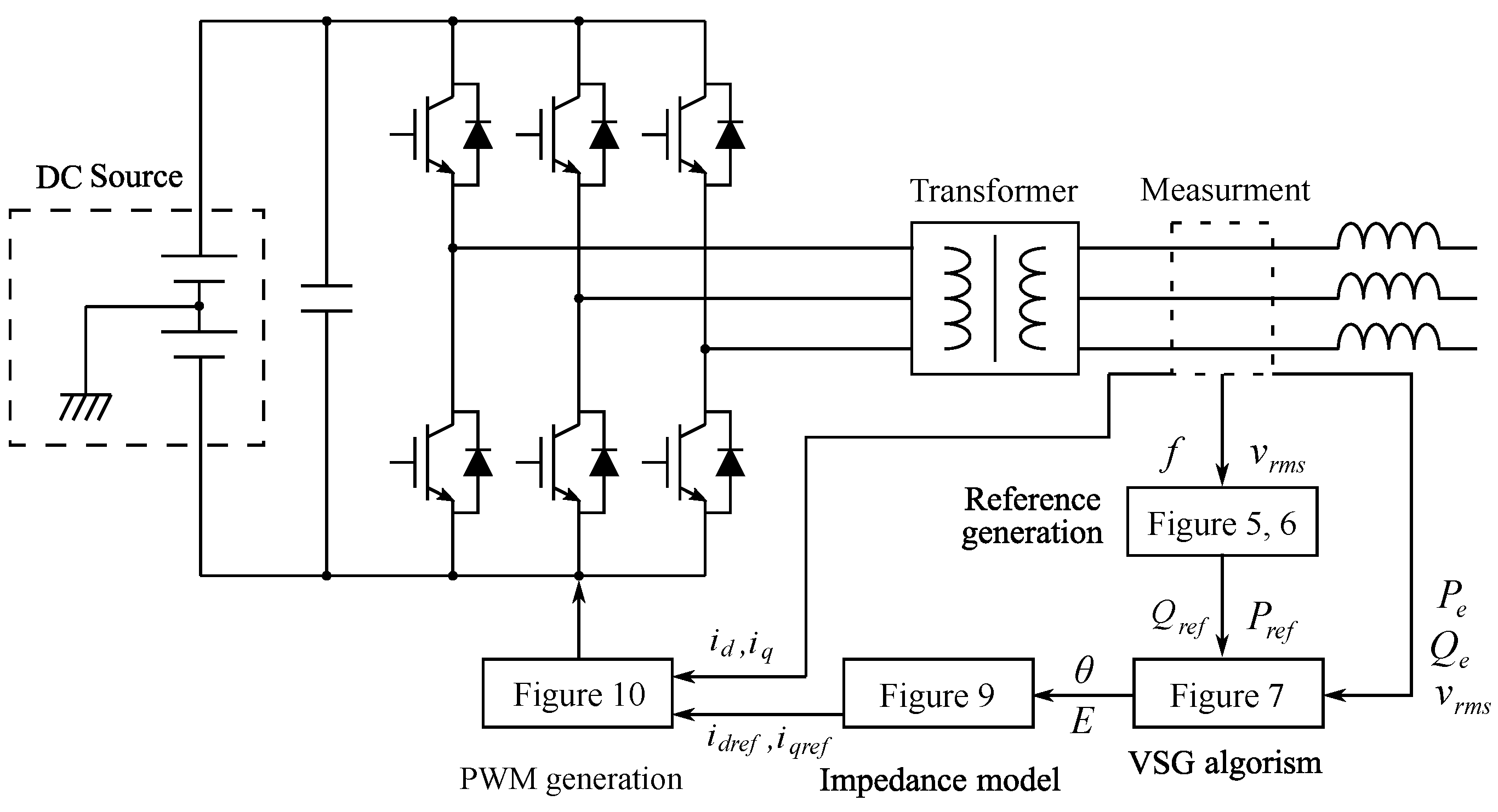
3. Virtual Synchronous Generator Model

The configuration diagram of the VSG is shown in Figure 3. The VSG consists of a DC voltage source and a three-phase full-bridge inverter. First, the frequency and voltage of the inverter are obtained, then active and reactive power references are generated. Next, the active and reactive power references are passed to a VSG control algorithm, which is obtained from the swing equations of a synchronous generator. Then, a virtual impedance model is used to determine d-axis current $i_d$ and q-axis current $i_q$. Finally, pulse width modulation (PWM) signals are generated by a PWM generator to input the inverter. In the following subsections, the details of these strategies are described.

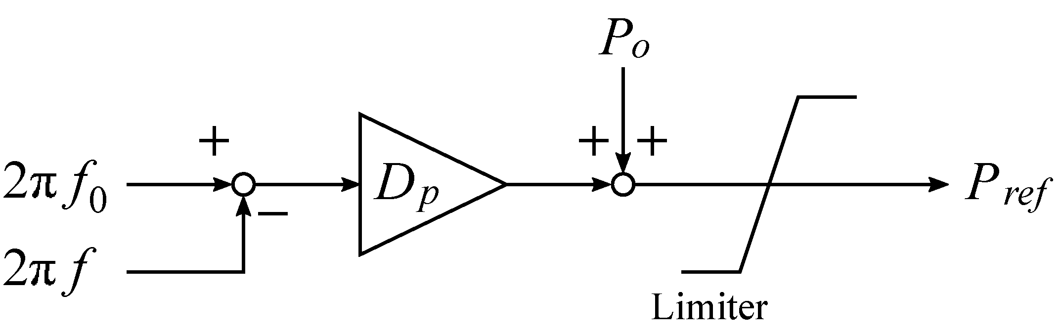
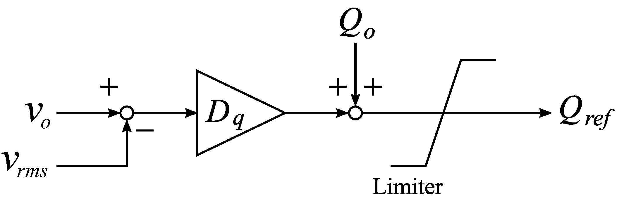
3.1. Active and Reactive Power Reference Generation Strategy

This subsection describes the generation method of the active and reactive power reference values. The block diagrams of the active and reactive power reference generation strategies are shown in Figure 4 and Figure 5, respectively.

In Figure 4, $f_o$ is the nominal frequency, f is the system frequency, $P_o$ is the nominal active power, $D_p$ is the Droop coefficient of active power for frequency deviation, and $P_{ref}$ is the active power reference. In Figure 5, $v_o$ is the nominal voltage, v is the RMS value of the system voltage, $Q_o$ is the nominal reactive power, $D_q$ is the Droop coefficient of reactive power for voltage deviation, and $Q_{ref}$ is the reactive power reference.

We assume that the system’s frequency is measured using a phase-locked loop (PLL) circuit, which tracks only the positive phase voltage of the system, thus providing stable phase and frequency measurements even in the event of voltage unbalance due to any incidents.

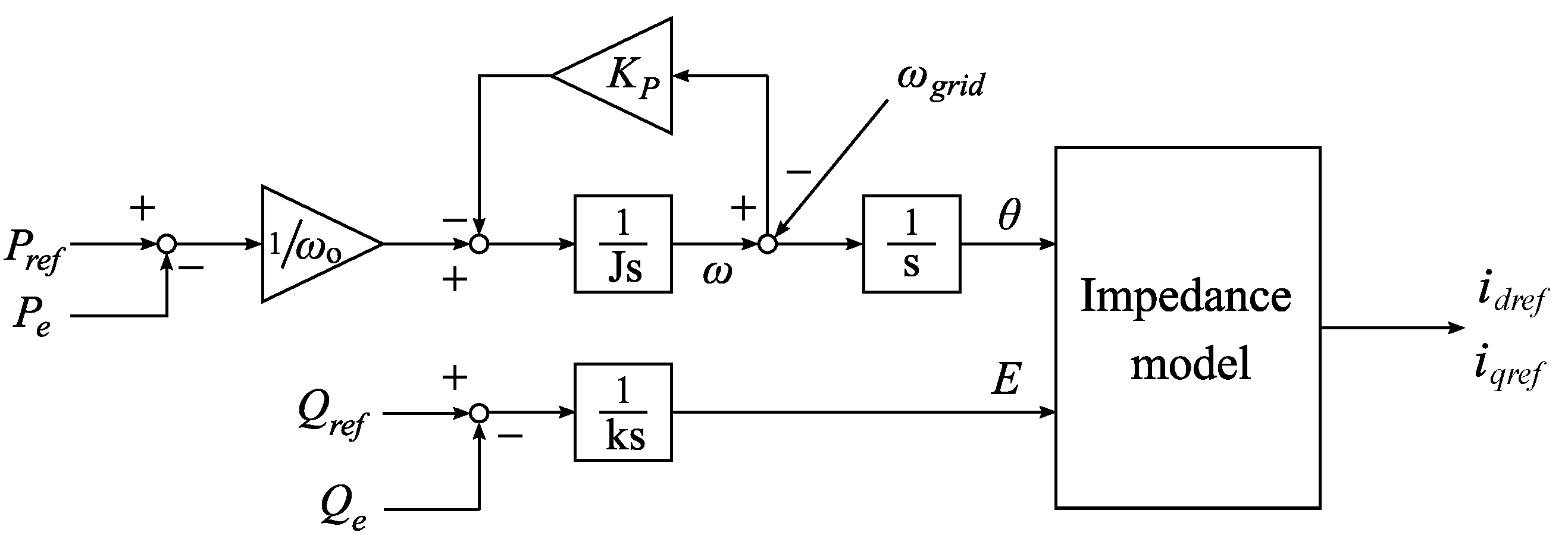
3.2. Virtual Synchronous Generator Control Strategy

The block diagram of the VSG control strategy is shown in Figure 6 [17]. The inertia of the VSG is simulated by the following equations [17]:

$$\begin{array}{ll}{T}_m-T_e-K_p\Delta \omega & =\frac{1}{\omega }(P_{ref}-P_e)-K_p(\omega -{\omega }_{grid})\\ & =J\frac{d\Delta \omega }{dt},\end{array}$$

(14)

$$\begin{array}{cc}\hfill & \frac{d\theta }{dt}=\omega ,\hfill \end{array}$$

(15)

$$\begin{array}{cc}\hfill & \frac{1}{k}\int (Q_{ref}-Q_e)+K_V(v_{rms}^{\prime }-v_{rms})dt=E.\hfill \end{array}$$

(16)

Here, $T_m$ and $T_e$ are the mechanical and electromagnetic torques, respectively; $P_e$ and $Q_e$ are the three-phase instantaneous active and reactive powers injected from the inverter, respectively; J is the virtual inertia coefficient of the inverter; $K_p$ is the virtual damping coefficient; $K_V$ is the voltage droop coefficient; k is the integral gain; and $v_{rms}$ is the RMS value of the voltage after passing through the filter. $P_e$, $Q_e$ and $v_{rms}$ are calculated as follows:

$$\begin{array}{cc}\hfill & P_e=v_d{i}_d+v_q{i}_q,\hfill \end{array}$$

(17)

$$\begin{array}{cc}\hfill & Q_e=v_d{i}_q-v_q{i}_d,\hfill \end{array}$$

(18)

$$\begin{array}{cc}\hfill & v_{rms}=\sqrt{v_d^2+v_q^2},\hfill \end{array}$$

(19)

where, using $dq$ transformation, $v_d$, $v_q$ and $i_d$, $i_q$, are calculated as

$$\begin{array}{cc}\hfill & \left[\begin{array}{c}{v}_d\\ v_q\end{array}\right]=\sqrt{\frac{3}{2}}\left[\begin{array}{ccc}cos\theta & cos(\theta -\frac{2\pi }{3})& cos(\theta -\frac{4\pi }{3})\\ -sin\theta & -sin(\theta -\frac{2\pi }{3})& -sin(\theta -\frac{4\pi }{3})\end{array}\right]\left[\begin{array}{c}{v}_a\\ v_b\\ v_c\end{array}\right],\hfill \end{array}$$

(20)

$$\begin{array}{cc}\hfill & \left[\begin{array}{c}{i}_d\\ i_q\end{array}\right]=\sqrt{\frac{3}{2}}\left[\begin{array}{ccc}cos\theta & cos(\theta -\frac{2\pi }{3})& cos(\theta -\frac{4\pi }{3})\\ -sin\theta & -sin(\theta -\frac{2\pi }{3})& -sin(\theta -\frac{4\pi }{3})\end{array}\right]\left[\begin{array}{c}{i}_a\\ i_b\\ i_c\end{array}\right].\hfill \end{array}$$

(21)

In a three-phase balanced system, the q-axis voltage is zero ($v_q=0$). Consequently, active power can be controlled by $i_d$ and reactive power by $i_q$.

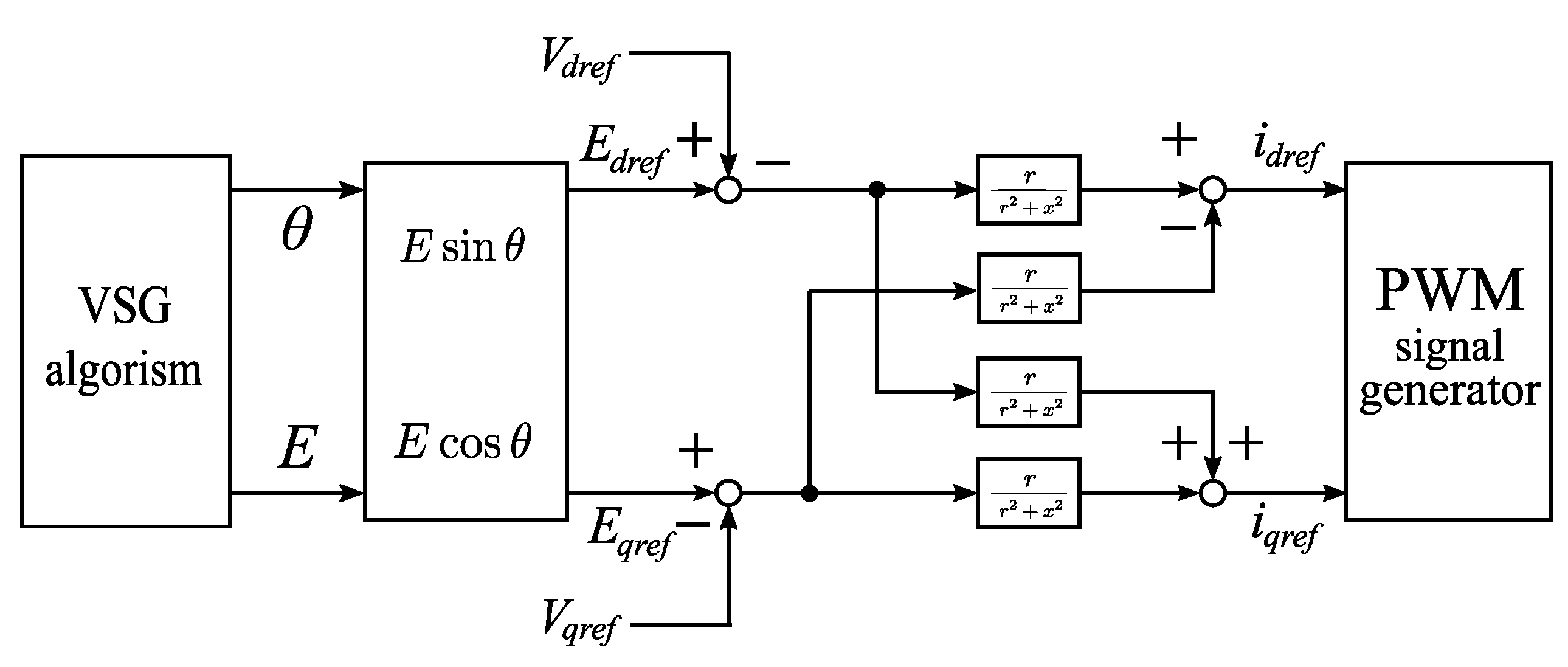
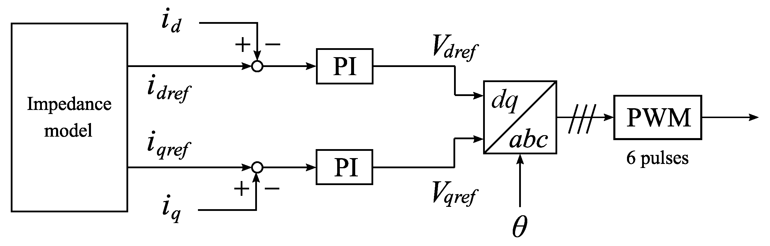
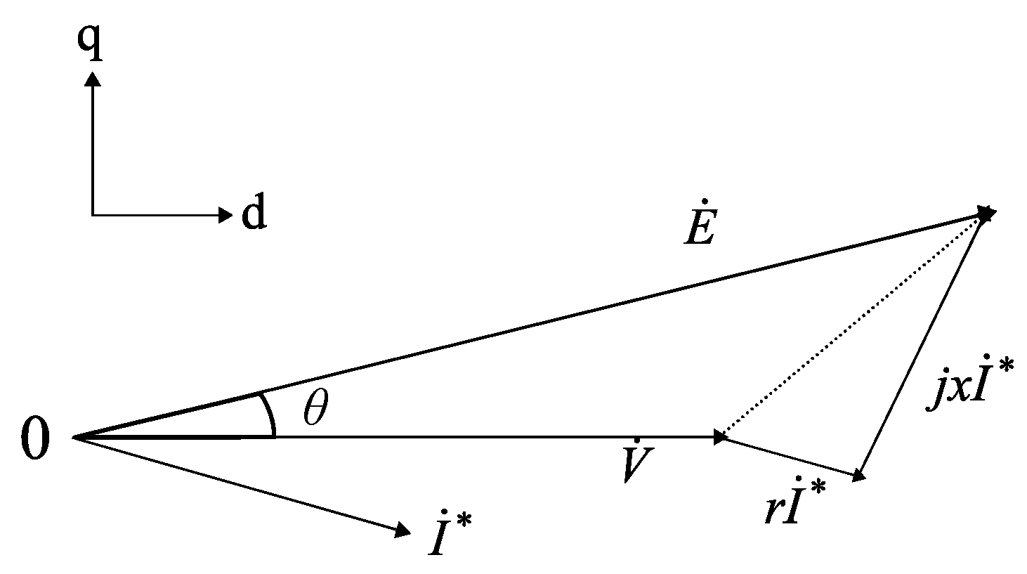
3.3. Virtual Impedance Model

This subsection describes the virtual impedance used to converting the phase difference $\theta$ and voltage E to $i_d$ and $i_q$ in the VSG control strategy of the previous subsection. This study adopts the concept of virtual impedance proposed in [18,19].

First, Figure 7 illustrates the phasor diagram of the virtual synchronous generator.

In Figure 7, $\dot{E}$ and $\dot{V}$ are the internal electromotive force and terminal voltage phasors in the generator, respectively; $\theta$ is the internal phase angle; r is the virtual resistance; x is the virtual reactance of the generator. Note that x is modeled as a constant. From Figure 7, the armature currents $i_d$ and $i_q$ can be expressed by

$$\begin{array}{cc}\hfill & \left[\begin{array}{c}{i}_d\\ i_q\end{array}\right]=Y\left\{\left[\begin{array}{c}{E}_d\\ E_q\end{array}\right]-\left[\begin{array}{c}{V}_d\\ V_q\end{array}\right]\right\},\hfill \end{array}$$

(22)

$$\begin{array}{cc}\hfill & Y=\frac{1}{r^2+x^2}\left[\begin{array}{cc}r& x\\ -x& r\end{array}\right]=\left[\begin{array}{cc}{Y}_{dd}& Y_{dq}\\ -Y_{dq}& Y_{dd}\end{array}\right],\hfill \end{array}$$

(23)

$$\begin{array}{cc}\hfill & \left[\begin{array}{c}{E}_d\\ E_q\end{array}\right]=\left|E\right|\left[\begin{array}{c}cos\theta \\ sin\theta \end{array}\right].\hfill \end{array}$$

(24)

From (22)–(24), the block diagram of the virtual impedance model is shown in Figure 8 [20].

In addition to the virtual impedance, the inverter has the actual impedance of the AC output filter. The actual impedance is more dominant in the high-frequency range, and the virtual impedance is more dominant in the low-frequency range.

After passing through this virtual impedance model, the PWM signal is generated. The block diagram of the PWM signal generation strategy is shown in Figure 9.

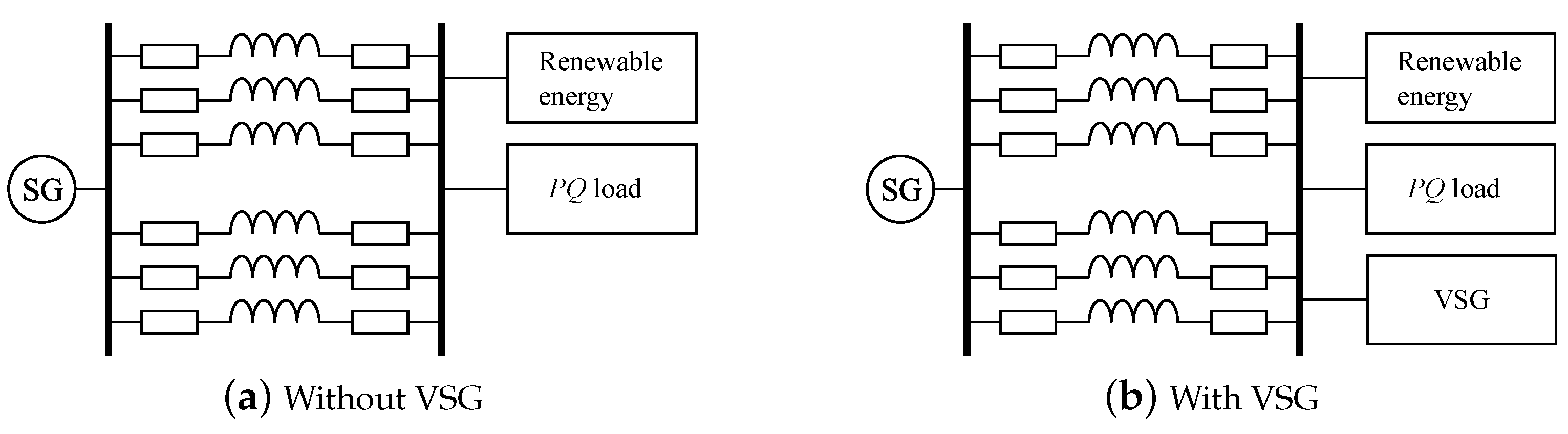
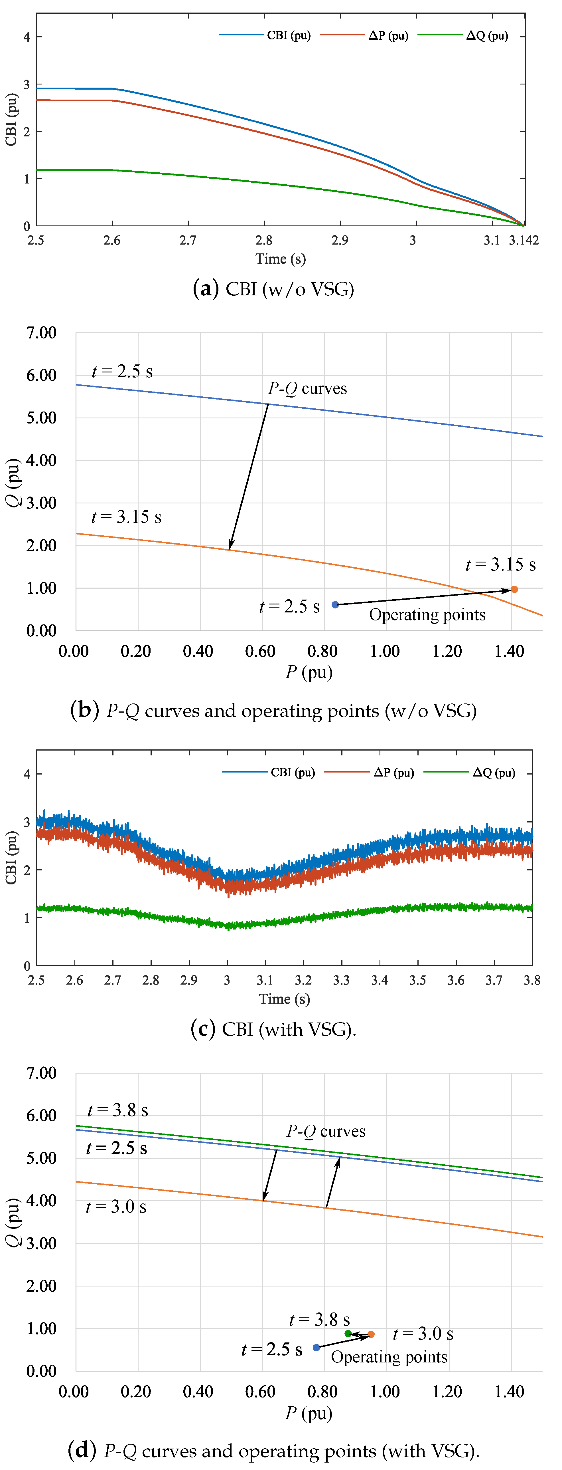
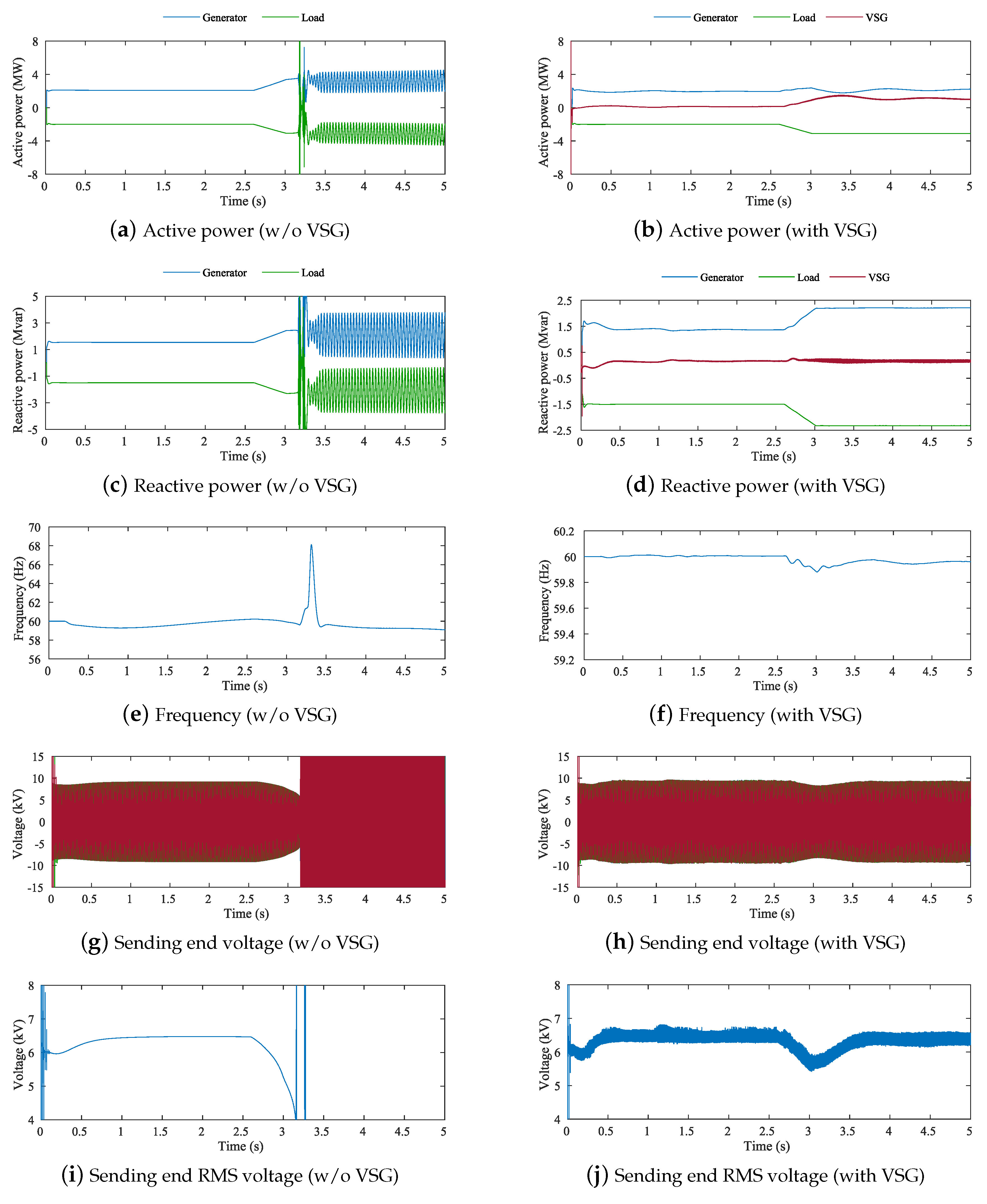
4. Simulation Results

In this study, we configure two remote island power system models with/without VSG. The models of the remote systems are shown in Figure 10. For a better understanding of the phenomenon, the remote island power systems are modeled as 2-bus systems. The systems are two-line three-phase AC systems. A $PQ$ load and renewable energy are connected to a synchronous generator located on the same island. Three-Phase Dynamic Load in Simulink^® is used as a load model.

Table 1. System parameters.

Description	Value
Sending end voltage	6.6 kV
Initial load	2.5 MW
Load power factor	0.8 pu
Frequency	60 Hz
Line resistance	1 $\mathsf{\Omega }$
Line inductance	0.001 H

and

Table 2. VSG parameters.

Description	Symbol	Value
Nominal active power	$P_o$	200 kW
Nominal reactive power	$Q_o$	150 kvar
Nominal frequency	$f_o$	60 Hz
Nominal voltage	$v_o$	6.6 kV
Droop coefficient of frequency	$D_p$	3,000,000
Droop coefficient of voltage	$D_q$	30.3
Virtual inertia coefficient	J	0.002
Virtual damping coefficient	$K_P$	0.2
Integral gain	k	20,000
Virtual resistance	r	2 $\mu \mathsf{\Omega }$
Virtual reactance	x	27 $\mathsf{\Omega }$

show the parameters of the power system and VSG models, respectively.

The following subsections provide case studies assuming two types of fault events. For each case study, the impact of VSG is examined by simulating and comparing both models, Figure 10a,b. In all cases, the simulations are run for $t=$ 0.0–5.0 s with a sampling period of 5 µs. We implemented the simulations on MATLAB/Simulink^®.

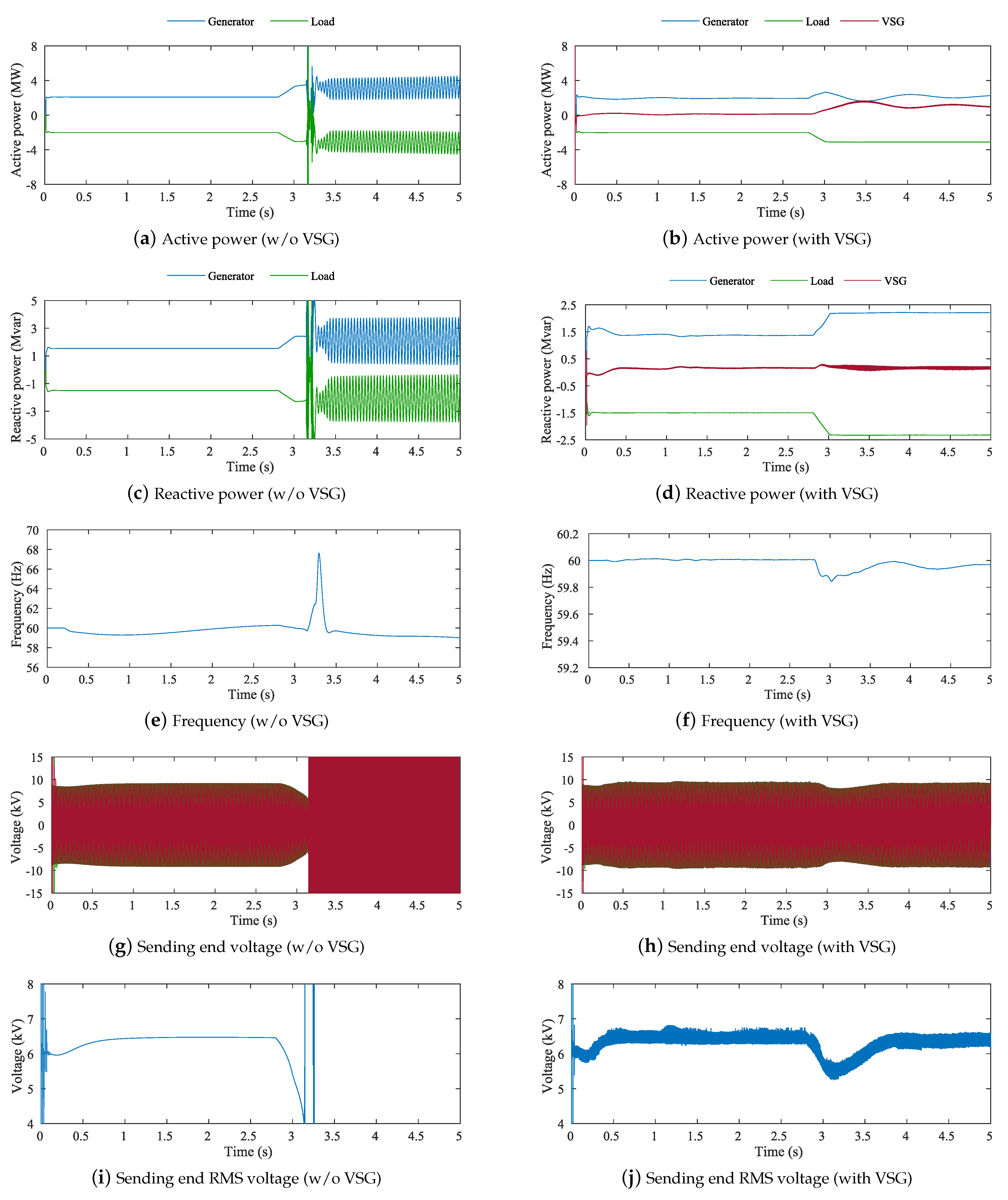
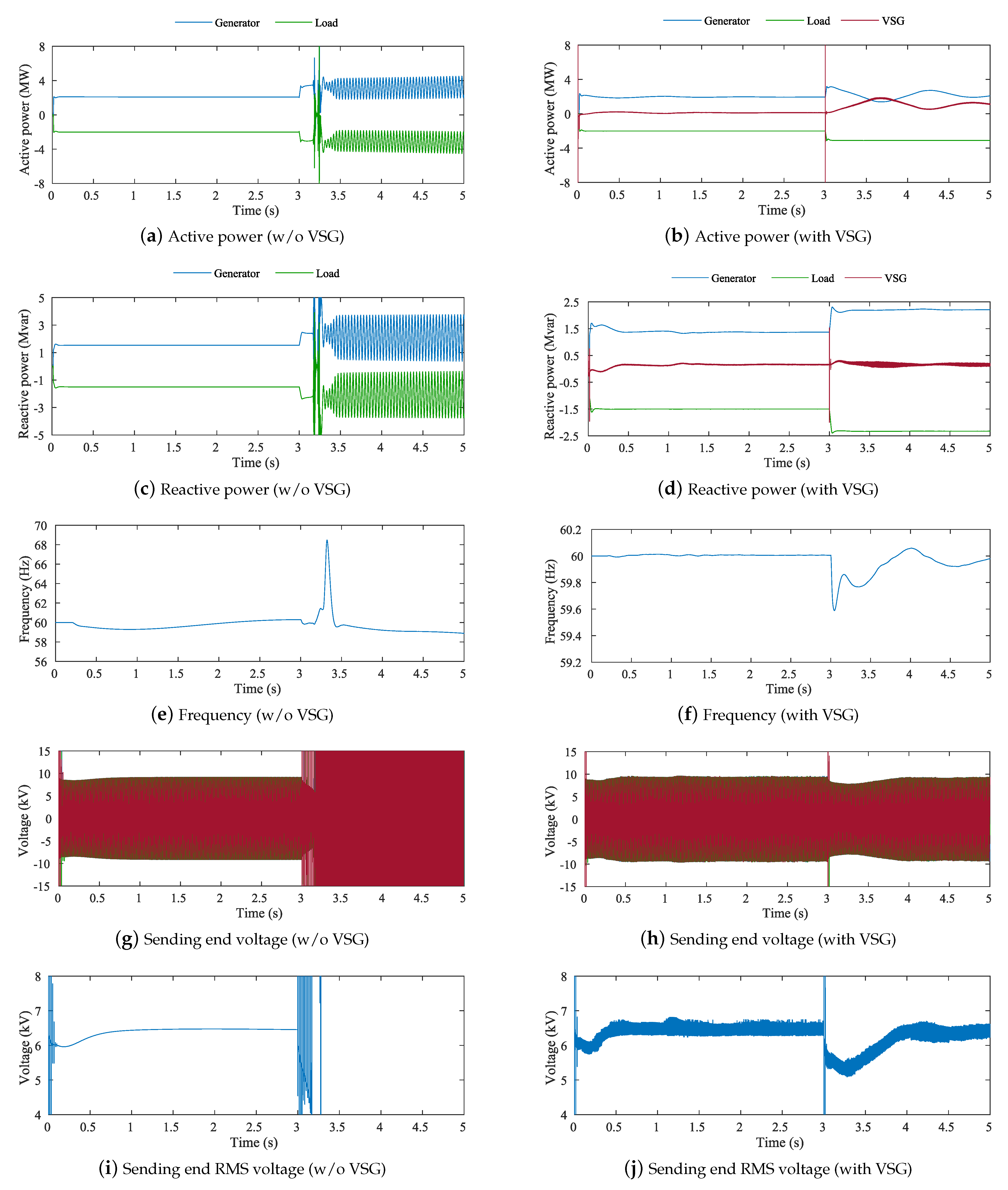
4.1. Case 1: Dynamic Voltage Stability during Renewable Energy Output Fluctuation

In Case 1, we discuss the dynamic voltage stability of the remote island power systems when the fluctuation of renewable energy output occurs. The three subcases listed below are examined to account for different fluctuation patterns.

Case 1.1:

Slow ramp-down of renewable energy output

Case 1.2:

Fast ramp-down of renewable energy output.

Case 1.3:

Sudden drop in renewable energy output.

In Case 1.1, ramp-down occurs from $t=2.6$ s, and in Case 1.2, ramp-down occurs from $t=2.8$ s, respectively. In Case 1.3, a sudden drop in renewable energy output occurs at $t=3.0$ s. In all subcases, the renewable energy output will decrease 0.05 pu from the initial state at $t=3.0$ s.

The simulation results of Case 1.1–1.3 are shown in Figure 11, Figure 12 and Figure 13, respectively. For Case 1.1 and 1.2, Figure 11g and Figure 12g show that each sending end voltage gradually decreases from each ramp-down point, and voltage collapse occurs between $t=$ 3.1–3.2 s. In contrast, Figure 11h and Figure 12h show that each voltage is recovered from $t=3.0$ s, and the voltage collapse does not occur with VSG.

On the other hand, for Case 1.3, Figure 13g shows that the voltage immediately starts to diverge intermittently from $t=3.0$ s, and voltage collapse occurs between $t=3.1$ s–$3.2$ s. Even in this case, Figure 13h shows the instantaneous overvoltage at $t=3.0$ s; however, the voltage collapse does not appear with VSG.

For each simulation, dynamic voltage stability is assessed using CBI. Figure 14 and Figure 15 show the time variation of CBI in Case 1.1 and 1.2. In Figure 14a and Figure 15a, we can observe that each CBI gradually decrease from each ramp-down point, and reaches 0 at $t=3.142$ s and $t=3.127$ s, respectively (i.e., voltage collapse has occurred). Compared to Case 1.1, Case 1.2 reached the voltage collapse slightly earlier. In contrast, Figure 14c and Figure 15c show that each CBI recover from $t=3.0$ s with VSG. These are consistent with the results shown in Figure 11 and Figure 12.

In Case 1.3, the intermittent overvoltages affect CBI calculation, but filtering the voltage by the moving median allows us to observe the trend of the CBI. In this case, the moving median at 5 ms intervals has been used, and calculated CBI is shown in Figure 16. Different from Case 1.1 and 1.2, Figure 16a shows that the CBI decreases sharply at $t=3.0$ s, and reaches 0 at $t=3.155$ s. On the other hand, Figure 16c shows the CBI drops once and then gradually recovers with VSG. These are consistent with the results shown in Figure 13.

Figure 14, Figure 15 and Figure 16 also visualize the time variation of both P-Q curves and operating points for further understanding. In Figure 14b, Figure 15b and Figure 16b, we observe that each P-Q curve and operating point are far enough distance from each other at $t=2.5$ s (i.e., CBI is large). However, after the fault, each operating points exceed each P-Q curve at each voltage collapse point. It implies that the operating points reach the unstable voltage region, as shown in Figure 2. On the other hand, in Figure 14d, Figure 15d and Figure 16d, each P-Q curve and operating point approach once, but then each P-Q curve and operating point move away from each other. This indicates that the voltage stability is recovered.

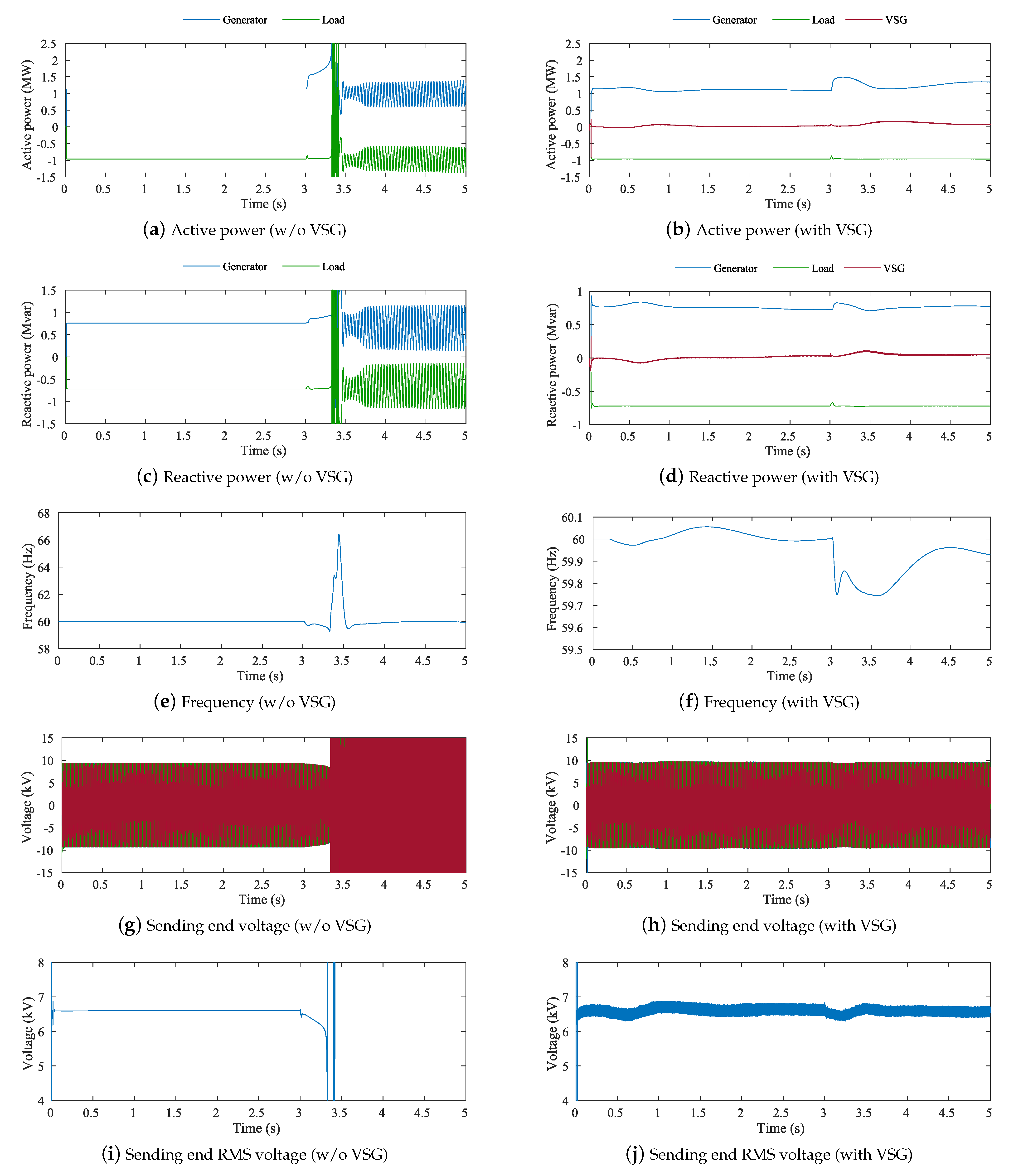
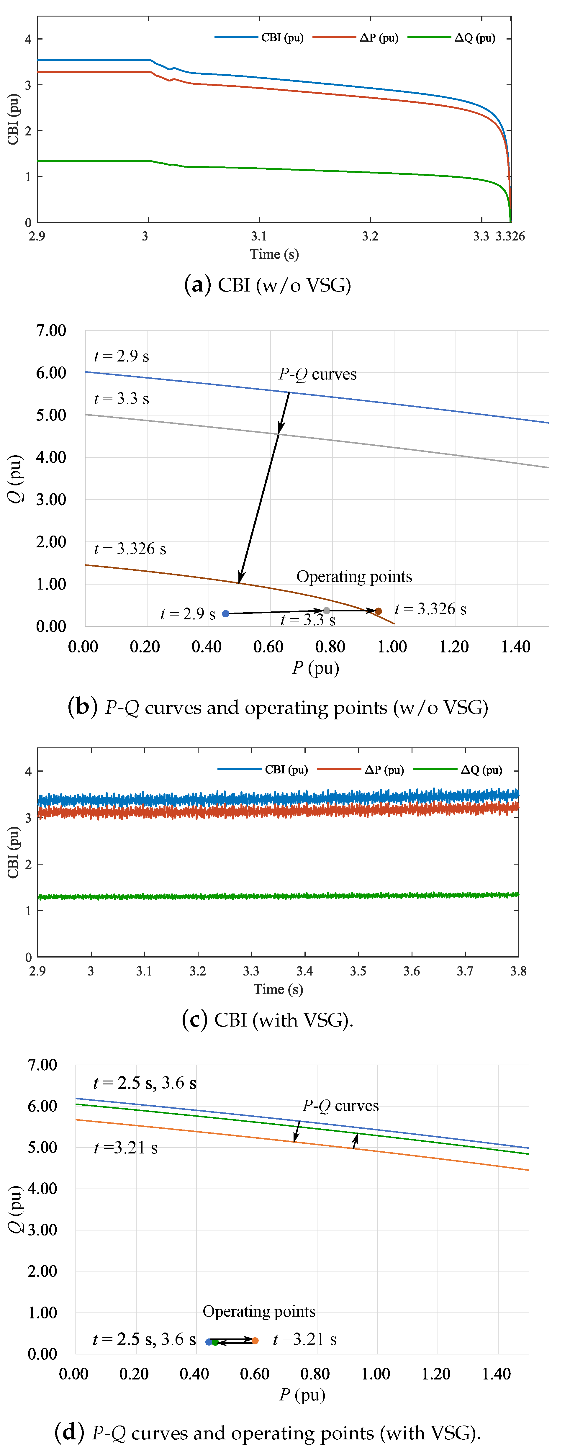
4.2. Case 2: Dynamic Voltage Stability during One-Line Outage of Transmission Line

In Case 2, we discuss the dynamic voltage stability of the remote island power systems when the one-line outage of the transmission line occurs. The one-Line outage occurs at $t=3.0$ s. The simulation results of Case 2 are shown in Figure 17. Figure 17g shows that the voltage gradually decreases from $t=3.0$ s and then rapidly moves towards voltage collapse around $t=3.3$ s. In contrast, Figure 17h shows that the voltage slightly fluctuates from $t=3.0$ s, but the voltage collapse does not occur with VSG.

For Case 2, dynamic voltage stability is assessed using CBI. Figure 18 shows the time variation of CBI in Case 2. In Figure 18a, we observe that the CBI gradually decreases from $t=3.0$ s and rapidly moves to 0 from $t=3.3$ s. In contrast, Figure 18c shows that the CBI is stable even if the fault is occurred. These are consistent with the results shown in Figure 17.

Figure 18 also visualizes the time variation of both P-Q curves and operating points for further understanding. In Figure 18b, the P-Q curve and operating point are far enough distance until $t=3.3$ s, but after $t=3.3$ s, the operating point and P-Q curve rapidly approach each other and reach to the unstable region at $t=3.326$ s. In contrast, Figure 18d shows that the P-Q curve and operating point always maintain the distance from each other.

5. Conclusions

This paper has aimed to validate the dynamic voltage stability assessment using CBI and investigated the impact of the VSG on voltage stability. For this purpose, we have presented case studies of fault events.

The case studies show that the CBI accurately detects the voltage collapse point even during fault events. It also confirms that the VSG suppresses the fast voltage collapse caused by fault events. From these results, we can conclude that the CBI can accurately assess the dynamic variation of voltage stability and that the VSG can contribute to maintaining the voltage stability against fault events.

Calculating the CBI based on $\Delta P$ and $\Delta Q$ makes it possible to know whether P or Q is closer to the stability limit. This implies that an online assessment of the CBI can be used to determine the optimal amount of compensation for the active and reactive power of the VSG, and this is our future work.

References

1. Shin, H.; Jung, J.; Oh, S.; Hur, K.; Iba, K.; Lee, B. Evaluating the Influence of Momentary Cessation Mode in Inverter-Based Distributed Generators on Power System Transient Stability. IEEE Trans. Power Syst. 2020, 35, 1618–1626. [Google Scholar] [CrossRef]
2. Drhorhi, I.; El Fadili, A.; El Kasmi, D.; Stitou, M. Evaluation of the moroccan electrical grid dynamic stability after large scale renewable energies integration. In Proceedings of the 3rd Renewable Energies, Power Systems and Green Inclusive Economy, REPS and GIE 2018, Casablanca, Morocco, 23–24 April 2018; Institute of Electrical and Electronics Engineers Inc.: Piscataway, NJ, USA, 2018. [Google Scholar] [CrossRef]
3. Wang, Y.; Chiang, H.D.; Wang, T. A two-stage method for assessment of voltage stability in power system with renewable energy. In Proceedings of the 2013 IEEE Electrical Power and Energy Conference, Halifax, NS, Canada, 21–23 August 2013; EPEC 2013. IEEE Computer Society: Piscataway, NJ, USA, 2013. [Google Scholar] [CrossRef]
4. Zhang, Y.; Zhou, Q.; Zhao, L.; Ma, Y.; Lv, Q.; Gao, P. Dynamic reactive power configuration of high penetration renewable energy grid based on transient stability probability assessment. In Proceedings of the 2020 IEEE 4th Conference on Energy Internet and Energy System Integration: Connecting the Grids Towards a Low-Carbon High-Efficiency Energy System, EI2 2020, Wuhan, China, 30 October–1 November 2020; Institute of Electrical and Electronics Engineers Inc.: Piscataway, NJ, USA, 2020; pp. 3801–3805. [Google Scholar] [CrossRef]
5. Radovanovic, A.; Naranjo Plaza, J.; Li, X.; Milanovic, J.V. The influence of hybrid renewable energy source plant composition on transmission system stability. In Proceedings of the IEEE PES Innovative Smart Grid Technologies Conference Europe, The Hague, The Netherlands, 26–28 October 2020; IEEE Computer Society: Piscataway, NJ, USA, 2020; pp. 584–588. [Google Scholar] [CrossRef]
6. Cheema, K.M.; Mehmood, K. Improved virtual synchronous generator control to analyse and enhance the transient stability of microgrid. IET Renew. Power Gener. 2020, 14, 495–505. [Google Scholar] [CrossRef]
7. Liu, J.; Yang, D.; Yao, W.; Fang, R.; Zhao, H.; Wang, B. PV-based virtual synchronous generator with variable inertia to enhance power system transient stability utilizing the energy storage system. Prot. Control Mod. Power Syst. 2017, 2, 1–8. [Google Scholar] [CrossRef]
8. Shi, R.; Zhang, X.; Hu, C.; Xu, H.; Gu, J.; Cao, W. Self-tuning virtual synchronous generator control for improving frequency stability in autonomous photovoltaic-diesel microgrids. J. Mod. Power Syst. Clean Energy 2018, 6, 482–494. [Google Scholar] [CrossRef] [Green Version]
9. Xu, Y.; Dong, Z.Y.; Meng, K.; Yao, W.F.; Zhang, R.; Wong, K.P. Multi-objective dynamic VAR planning against short-term voltage instability using a decomposition-based evolutionary algorithm. IEEE Trans. Power Syst. 2014, 29, 2813–2822. [Google Scholar] [CrossRef]
10. Moghavvemi, M.; Omar, F. Technique for contingency monitoring and voltage collapse prediction. IEE Proc.-Gener. Transm. Distrib. 1998, 145, 634–640. [Google Scholar] [CrossRef]
11. Moghavvemi, M.; Faruque, M.O. Technique for assessment of voltage stability in Ill-conditioned radial distribution network. IEEE Power Eng. Rev. 2001, 21, 58–60. [Google Scholar] [CrossRef]
12. Musirin, I.; Rahman, T.K. Estimation of maximum loadability in power systems by using fast voltage stability index. Int. J. Power Energy Syst. 2005, 25, 181–189. [Google Scholar] [CrossRef]
13. Yazdanpanah-Goharrizi, A.; Asghari, R. A Novel Line Stability Index (NLSI) for Voltage Stability Assessment of Power Systems. In Proceedings of the 7th WSEAS International Conference on Power Systems, Beijing, China, 15–17 September 2007; pp. 164–167. [Google Scholar]
14. Lim, Z.J.; Mustafa, M.W.; Bt Muda, Z. Evaluation of the effectiveness of voltage stability indices on different loadings. In Proceedings of the 2012 IEEE International Power Engineering and Optimization Conference, PEOCO 2012-Conference Proceedings, Melaka, Malaysia, 6–7 June 2012; pp. 543–547. [Google Scholar] [CrossRef] [Green Version]
15. Furukakoi, M.; Adewuyi, O.B.; Shah Danish, M.S.; Howlader, A.M.; Senjyu, T.; Funabashi, T. Critical Boundary Index (CBI) based on active and reactive power deviations. Int. J. Electr. Power Energy Syst. 2018, 100, 50–57. [Google Scholar] [CrossRef]
16. Kamel, M.; Karrar, A.A.; Eltom, A.H. Development and Application of a New Voltage Stability Index for On-Line Monitoring and Shedding. IEEE Trans. Power Syst. 2018, 33, 1231–1241. [Google Scholar] [CrossRef] [Green Version]
17. Zheng, T.; Chen, L.; Guo, Y.; Mei, S. Comprehensive control strategy of virtual synchronous generator under unbalanced voltage conditions. IET Gener. Transm. Distrib. 2018, 12, 1621–1630. [Google Scholar] [CrossRef]
18. Hirase, Y.; Sugimoto, K.; Sakimoto, K.; Ise, T. Analysis of Resonance in Microgrids and Effects of System Frequency Stabilization Using a Virtual Synchronous Generator. IEEE J. Emerg. Sel. Top. Power Electron. 2016, 4, 1287–1298. [Google Scholar] [CrossRef]
19. Hirase, Y.; Abe, K.; Sugimoto, K.; Sakimoto, K.; Bevrani, H.; Ise, T. A novel control approach for virtual synchronous generators to suppress frequency and voltage fluctuations in microgrids. Appl. Energy 2018, 210, 699–710. [Google Scholar] [CrossRef]
20. Hirase, Y.; Abe, K.; Sugimoto, K.; Shindo, Y. A grid-connected inverter with virtual synchronous generator model of algebraic type. IEEJ Trans. Power Energy 2013, 184, 371–380. [Google Scholar] [CrossRef]
Figure 1. 2-bus transmission line model. (From Ref. [15] ).
Energies 14 05851 g001
Figure 2. P-Q characteristics. (From Ref. [15]).
Energies 14 05851 g002
Figure 3. Overall VSG configuration.
Energies 14 05851 g003
Figure 4. Block diagram of active power reference generation strategy.
Energies 14 05851 g004
Figure 5. Block diagram of reactive power reference generation strategy.
Energies 14 05851 g005
Figure 6. Block diagram of VSG control strategy.
Energies 14 05851 g006
Figure 7. Phasor diagram of virtual synchronous generator.
Energies 14 05851 g007
Figure 8. Block diagram of virtual impedance model.
Energies 14 05851 g008
Figure 9. Block diagram of PWM signal generation strategy.
Energies 14 05851 g009
Figure 10. Remote island power system model with/without VSG.
Energies 14 05851 g010
Figure 11. Simulation results of Case 1.1 with/without VSG.
Energies 14 05851 g011
Figure 12. Simulation results of Case 1.2 with/without VSG.
Energies 14 05851 g012
Figure 13. Simulation results of Case 1.3 with/without VSG.
Energies 14 05851 g013
Figure 14. Critical boundary index (CBI) in Case 1.1 with/without VSG.
Energies 14 05851 g014
Figure 15. Critical boundary index (CBI) in Case 1.2 with/without VSG.
Energies 14 05851 g015
Figure 16. Critical boundary index (CBI) in Case 1.3 with/without VSG.
Energies 14 05851 g016
Figure 17. Simulation results of Case 2 with/without VSG.
Energies 14 05851 g017
Figure 18. Critical boundary index (CBI) in Case 2 with/without VSG.
Energies 14 05851 g018