Data-Driven Prognostics of the SOFC System Based on Dynamic Neural Network Models

Abstract

Prognostics technology is important for the sustainability of solid oxide fuel cell (SOFC) system commercialization, i.e., through failure prevention, reliability assessment, and the remaining useful life (RUL) estimation. To solve SOFC system issues, data-driven prognostics methods based on the dynamic neural network (DNN), one of non-linear models, were investigated in this study. Based on DNN model types, the neural network autoregressive (NNARX) model with external inputs, the neural network autoregressive moving average (NNARMAX) model with external inputs, and the neural network output error (NNOE) were utilized to predict the degradation trend and estimate the RUL. First, the degradation trend prediction was executed to evaluate the correctness of the proposed DNN model structures in the first learning phase. Then, the RUL was estimated on the basis of the degradation trend of the NN models in the second inference phase. The comparison test results show the prediction accuracy of the NNARX model is higher and the RUL estimation can be given within a smaller relative error than the NNARMAX and NNOE models. The evaluation criteria of the root mean square error and mean absolute error of the NNARX model are the smallest among these three models. Therefore, the proposed NNARX model can effectively and precisely provide degradation trend prediction and RUL estimation of the SOFC system.

1. Introduction

Renewable energy technologies are being heavily studied due to the depletion of fossil energy reserves and global environmental issues. Solid oxide fuel cell (SOFC) technology is a renewable and sustainable source of energy; its advantages include low noise, near zero emissions, superior energy efficiency, and high power density [1,2]. Nevertheless, the performance of a SOFC system can be easily affected by inadequate operation, impure inlet gases, and aging [3]. These degradation mechanisms are generated by uncertain complexities and environment conditions, which is why durability and reliability are obstacles to the large-scale deployment of SOFC systems [4].

Due to the durability, reliability, and cost (i.e., of long-life) issues of SOFC systems, effective maintenance strategies are important. Various strategies have been conducted to evaluate system conditions and to avoid high cost maintenance procedures. Prognostics and health management (PHM) is a novel maintenance strategy and is receiving increasing attention [5]; it offers cost-effective prediction and detection to improve availability, reliability, and security of the system. The PHM of the SOFC system uses real measurement data to predict the health degradation trend and estimate the residual of life or remaining useful life (RUL) to effectively prolong the lifespan of the SOFC system. In the process of PHM, prognostics technology plays an important role in predicting future conditions, and for RUL to be functional [6].

Currently, various prognostics methods are being studied to predict the degradation trend and estimate RUL, and can be separated into three categories: physics-based, data-driven, and hybrid [7,8]. The physics-based methods, also called fault physics and white box models, describe the phenomenon of system and failure models using empirical or mathematical relations. The comprehensive reviews of mathematical modeling of SOFCs are available to predict the fuel cell behaviors [9,10,11]. The advantages of these methods are that they are able to identify compositions according to their specifications [12], such as material properties, geometrical features, degradation of electrochemistry phenomena, etc. A physics-based method is suitable for better understanding the aging phenomena of the SOFCs. However, because it is not easy to build an accurate model, a proper mathematical representation has not been conducted due to the lack of failure mechanisms for complex SOFC systems. Hence, a physics-based method may not be appropriate to describe the physical degradation mechanism since assumptions, errors, and uncertainties are made in modeling [13]. In other words, the computationally complex and insufficiently accurate knowledge of degradation physics leads to increased uncertainty in prognosis of the SOFC system.

In contrast, data-driven methods can be considered as black-box models that learn the system behavior directly from the collected monitoring measurement data, without system expertise and complex physical equations [14]. This type of method converts the experimental data of state monitoring and historical data into appropriate information and system degradation behavioral models [15]. Data-driven methods generally use different machine learning approaches to either predict the degradation trend or estimate the RUL, and are particularly suitable for the SOFC complex system even though degradation mechanisms are not well understood. From the open literature, the traditional data-driven methods of nonlinear systems generally include the regression model [16], the Wiener process, gamma process [17], stochastic filtering model, risk-based covariance model, hidden Markov model, and semi-hidden Markov Model [18]. The advantage of a data-driven method is that it has strong, nonlinear imitation, and is easily implemented. Hybrid methods are used by integrating physics-based and data-driven methods, taking advantage of both methods and, hence, solving the shortcomings of a single method. Combining physics-based and data-driven methods allows for cumulating their advantages, but there are drawbacks; i.e., hybrid methods still need a lot of computing time to compare the physics-based and data-driven methods [19]. According to the above advantages and disadvantages of the different prognostics methods, the study proposes a data-driven prognostics method for the SOFC system.

From the literature review, to the best of the authors’ knowledge, the current prognostics methods for fuel cells mostly focus on proton exchange membrane fuel cell (PEMFC) systems. In addition, the degradation trend of performance and RUL estimation of the SOFC system, using effective data-driven methods, have not been published in the literature. Recently, due to the rapid development of algorithms in the semiconductor sector, data-driven methods based on artificial neural network (ANN) methodologies are attracting increasing attention in the engineering and applied science fields [20,21,22]. The ANN methods, especially the dynamic neural network (DNN) model, can effectively describe the complex nonlinear characteristics between inputs and outputs, such as the SOFC system. The advantage of the DNN model is the ability to use previous state memory to deal with nonlinear problems; it is particularly useful in solving time series prognostics topics [23,24,25].

The present work, conducted with DNN models, focuses on the neural network autoregressive exogenous (NNARX) input model, the neural network autoregressive moving average with exogenous (NNARMAX) input model, and the neural network output error (NNOE) model, to investigate the degradation trend prediction and the RUL estimation of the SOFC system. First, the experimental raw data preprocessing was performed to eliminate the unreliable measurement data to reduce the computational complexity by the locally weighted scatterplot smoothing (LOWESS) technique. Second, NNARX, NNARMAX, and NNOE models were built to predict the voltage degradation of SOFC performance with evaluation criteria. Finally, the RUL of the SOFC system was estimated based on the critical threshold. Moreover, the results of the degradation trend prediction and RUL estimation were compared with three methods to show feasibility.

The remainder of this paper is organized as follows. Section 2 presents the long-term experiment setting and data implementation of the SOFC system. Section 3 presents the whole prognostics framework based on NNARX, NNARMAX, and NNOE for the SOFC system. In Section 4, the prognostic framework based on DNN methods are presented. The comparison results and discussion for different prognostics methods are presented in Section 5. Finally, the concluding remarks are demonstrated in Section 6.

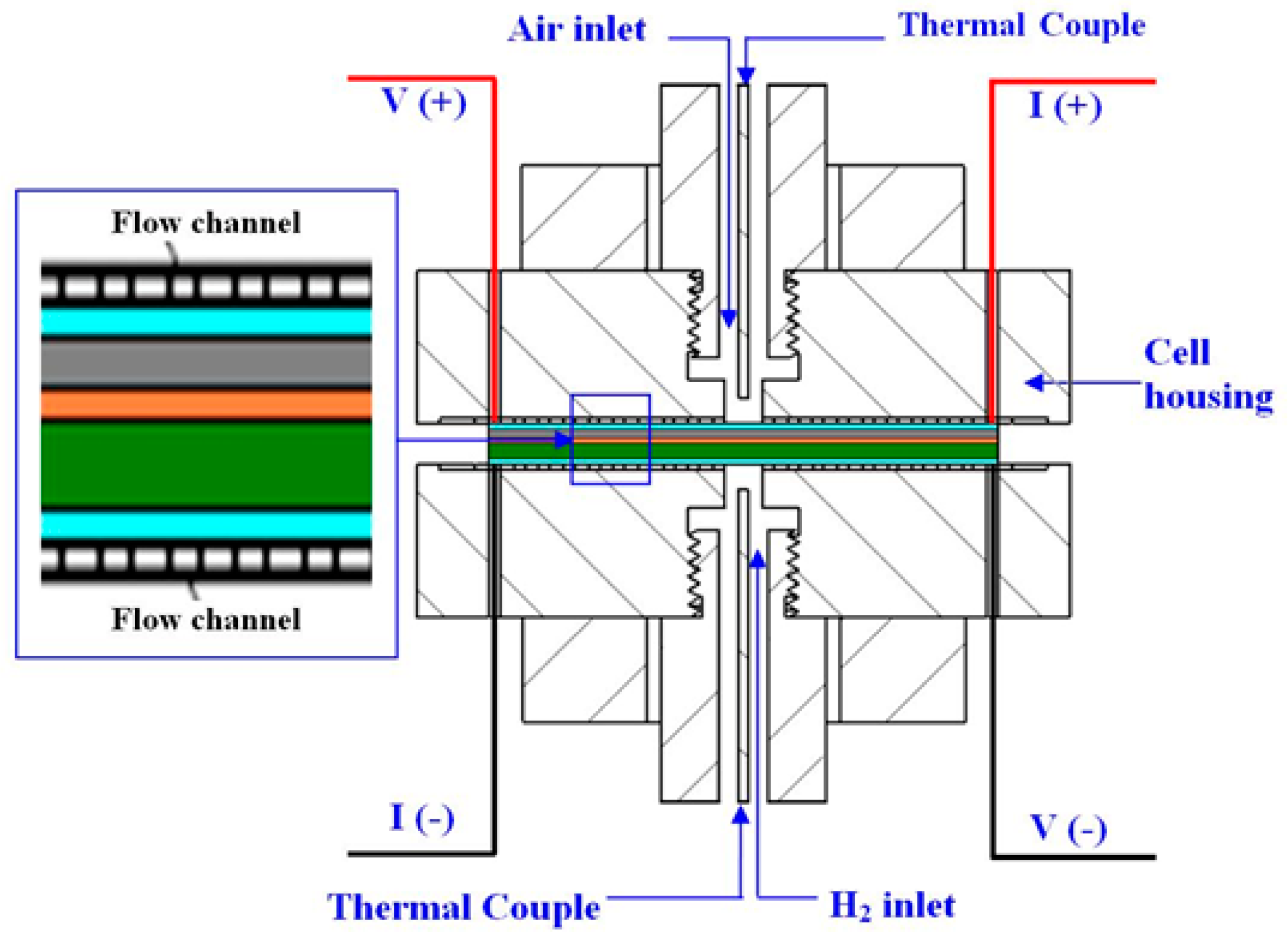
2. Experiment Setting and Data Implementation

In this section, the experimental setting and data implementation of the commercial anode-supported cell (ASC) type of the SOFC system were derived in the first. Specifically, the aging effects for the long-term degradation test and thermal cycle test were carried out based on the non-sealed cell test facility, as shown in Figure 1 [26]. The test cell of the SOFC was placed between the fuel and oxidant housings to separate the gases and facilitate electricity generation, and mixed gases burning occurred when the gases escaped the region of the cell. In the facility of SOFC system, hydrogen and nitrogen can be supplied on the anodic side and, at the same time, oxygen and air can be provided on the cathode side, respectively. The cell housing test bench consisted of flow field plates that connected to the control system through a metal pipe to provide fuel and oxidants, thermocouples, gas pipes, current collectors, and voltage and current wires, allocating with a metal net collecting current.

The test environment conditions and recording of the test data can be provided by the control system. The key compositions of the SOFC cell, NiO/YSZ, YSZ, and LSC, are included in different planar structure layers of the anode, electrolyte, and cathode, with a total thickness of 550 μm, an active area of $9\times 9$ cm², and a size of $10\times 10$ cm². The main compositions and thicknesses of the cell, manufactured commercially, are listed in

Table 1. Main composition and thickness of the commercial SOFC cell.

Layer	Composition/Thickness
Anode composition	NiO/YSZ (12$\mathsf{\mu }$m)
Anode support	NiO/YSZ (500$\mathsf{\mu }$m)
Cathode composition	LSC (20–30$\mathsf{\mu }$m)
Electrolyte composition	YSZ (3$\mathsf{\mu }$m)

. In order to obtain a higher electrical output, the operating temperature of the SOFC system in this experiment was set to 700 °C. The long-term stability is the main factor and the most important characteristic for SOFC commercial life to evaluate the durability. We investigated the influence of the flow rate of gases for the long-term test (5000 h) at operating temperatures heated up to 700 °C. The first 3000 h of the long-term test of a standard operating procedure (SOP) was operated with cathode air and anode hydrogen supplied by a constant gas flow rate of 800 to 2000 cm³/min, respectively. Afterward, the polarization curve performances were performed under a current density of 400 mA/cm².

To determine the influence of the reduced flow rate on cell performance and durability, the long-term test with a reduced flow rate, for 200 h, was carried out after a 3000 h SOP long-term test. The flow rates of the cathode air and anode hydrogen were reduced within 500 and 1500 cm³/min, respectively, after the SOP long-term test was held for 2000 h. From the previous results of the SOP test, the long-term durability of the open current voltage (OCV) was higher than the basic value. However, the OCV of the latter test, after 2000 h, was less than the former SOP test. The reason for the performance degradation is because the internal gas partial pressure became irreversible. More detailed results and analysis about the SOFC experiment can be found in previous published literature [27,28]. Considering the most important and available degradation characteristics, the output voltage of the SOFC system, as a health indicator, is a suitable index to describe the degradation of performance [29].

3. Considered Theory

The reliable and accurate prognostics methods play an important role in the life and maintenance costs of the SOFC system by predicting the future performance and RUL. In this study, the DNN nonlinear time-series model structures, such as NNARX, NNARMAX, and NNOE models, were employed to establish the long-term degradation trend prediction and the RUL estimation for the SOFC performance. In basic DNN networks architecture, the model outputs depend on the current input as well as the current or previous inputs, outputs, or states of the network, as presented in Figure 2. The advantage of the proposed prognostics method can build the complex relationship and the ability to extract the implicit nonlinear characteristics in such a multivariate SOFC system. In addition, they also have good “learning” sequential, time-varying capacity, and generalization capabilities of prognostics algorithms/prognostics performance. Thanks to the superior performance of the nonlinear DNN methods, NNARX, NNARMAX, and NNOE models were applied in the present research for prognostics, the long-term performance degradation trend, and the RUL estimation of the SOFC system.

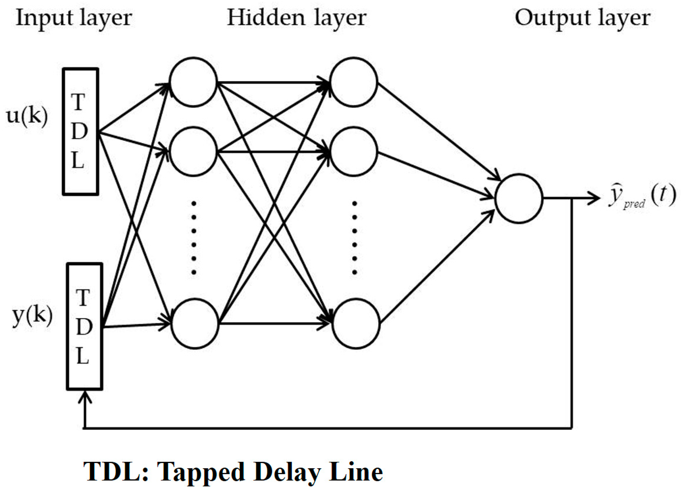
3.1. Model Development

The nonlinear time-series DNN models are used to construct networks for prognostics of the SOFC system and can be expressed by the general input–output empirical form as below [23]:

$$A\left(q\right)y\left(t\right)=\frac{B\left(q\right)}{C\left(q\right)}u\left(t-n_k\right)+\frac{D\left(q\right)}{E\left(q\right)}e\left(t\right)$$

(1)

where $q$ is negative shift operator, and the A(q), B(q), C(q), D(q), and E(q) are polynomials structures, which present different model types. For the ARX model, the terms of polynomial C(q), D(q), and E(q) are set to 1; the ARMAX model, the C(q), and E(q) are set to 1; the OE model, the A(q), D(q), and E(q) are also set to 1. The input–output model can be presented in a regression form within A(q) in q⁻¹:

$$\widehat{y}={\varnothing }^{T}X\left(t\right)$$

(2)

where $\widehat{y}$ is the model predicted output and ${\varnothing }^T$ is the dynamic neural unit model type. According to the different model types, the dynamic neural unit structure parameter of X(t) is constructed by:

(1)

The B polynomial is related to the control signal.

$$u\left(t-i\right),i=1,\dots ,n_b$$

(3)

(2)

The A polynomial is related to the output of the measurement.

$$y\left(t-i\right),i=1,\dots ,n_a$$

(4)

(3)

The $\widehat{y}\left(k-i\right)$ is related to the simulated outputs from the past u(k), associated with the C polynomial.

(4)

The predicted errors are associated with the D polynomial.

$$e\left(t-i\right)=y\left(t-i\right)-\widehat{y}\left(t-i\right)$$

(5)

The relationship of the input–output nonlinear models can be expressed as follows:

$$X\left(t\right)=\left[y\left(t-1\right),\dots ,y\left(t-n_a\right),u\left(t-1\right),\dots ,u\left(t-n_b\right)\right] \mathrm{for} \mathrm{ARX} \mathrm{model}$$

(6)

$$X\left(t\right)=\left[\begin{array}{c}y\left(t-1\right),\dots ,y\left(t-n_a\right),u\left(t-n_k\right),\dots ,u\left(t-n_b\right)\\ {\epsilon }_u\left(t-1\right),\cdots ,{\epsilon }_u\left(t-n_e\right)\end{array}\right] \mathrm{for} \mathrm{ARMAX} \mathrm{model}$$

(7)

$$X\left(t\right)=\left[\widehat{y}\left(t-1\right),\dots ,\widehat{y}\left(t-n_a\right),u\left(t-1\right),\dots ,u\left(t-n_b\right)\right] \mathrm{for} \mathrm{OE} \mathrm{model}$$

(8)

where u(t) is the control input, y(t) is the measured output,, and ε(t) is the white noise disturbance. The n_a is the output order of model, n_b is the input order of model, n_k is past time delay, and n_e is the noise order of the model. The dynamic neural unit of the nonlinear DNN model can be summarized as follows:

$$\begin{gathered} \mathrm{NNARX}=\left[\begin{array}{ccc}{n}_a& n_b& n_k\end{array}\right] \\ \mathrm{NNARMAX}=[\begin{array}{ccc}{n}_a& n_b& \begin{array}{cc}{n}_c& n_k\end{array}\end{array}] \\ \mathrm{NNOE}=\left[\begin{array}{ccc}{n}_a& n_b& n_k\end{array}\right] \end{gathered}$$

(9)

3.2. Learning with Backpropagation (BP) Method

Parameter estimation is a process involving mathematical model optimization based on proposed neural network nonlinear autoregressive models of the SOFC system. The principle of the parameter estimation is to select the accurate method or the prediction criterion to be minimized. The backpropagation neural network (BPNN), as the most commonly used learning algorithm, is a multilayer perceptron (MLP) neural network; it has the ability to model simple (as well as very complex) functional relationships [30]. Therefore, the customary to apply three-layer feedforward neural network structures with input layer, hidden layer, and output layer is conducted. The predicted output model forms within BPNN, confined in one hidden layer, with a hyperbolic tangent function (f) and linear function (F) used in the hidden and output layer, derived as follows:

$${\widehat{y}}_i\left(w,W\right)=F_i\left\{{\displaystyle \sum }_{j=1}^q{W}_{ij}{h}_j\left(w\right)+W_{i0}\right\}=F_i\left\{{\displaystyle \sum }_{j=1}^q{W}_{ij}{f}_j\left({\displaystyle \sum }_{l=1}^m{w}_{jl}{z}_l+w_{j0}\right)+W_{i0}\right\}$$

(10)

The weights specified by the unknown parameter vector θ or in terms of the matrices, w and W, are adjustable for the network parameters, which is determined by the training process. The objective of the training network is to minimize error functions between predictions and measurements.

The prediction error is based on the introduction of a measurement of closeness in terms of a normalized sum square error criterion. An empirical equation for the determination of hidden neurons used in a previous study is expressed as follows:

$$h_{nn}=\sqrt{m+n}+\alpha$$

(11)

where h_nn, m, and n are the numbers of hidden neurons, inputs, and outputs, respectively; $\alpha$ represents a constant from 1 to 10. Moreover, from the analysis of results, according to our published literature [31], the hidden neuron number of 10 is selected and used in the following analysis.

4. Prognostic Framework Based on DNN Methods

The proposed prediction of the degradation trend and estimate of the RUL framework of the SOFC system, based on the DNN model, are shown in Figure 3, and described in detail according to processes in the following.

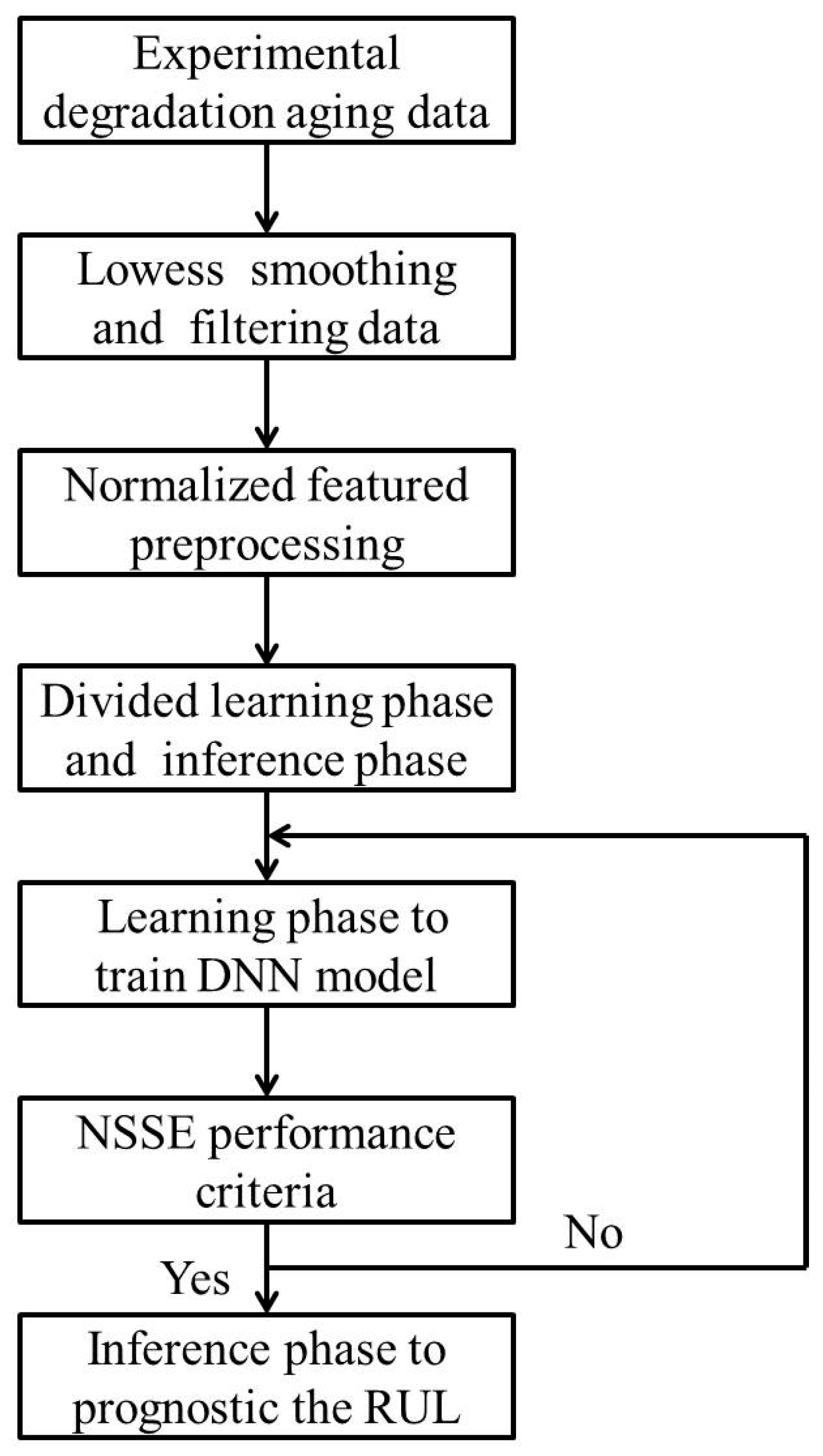
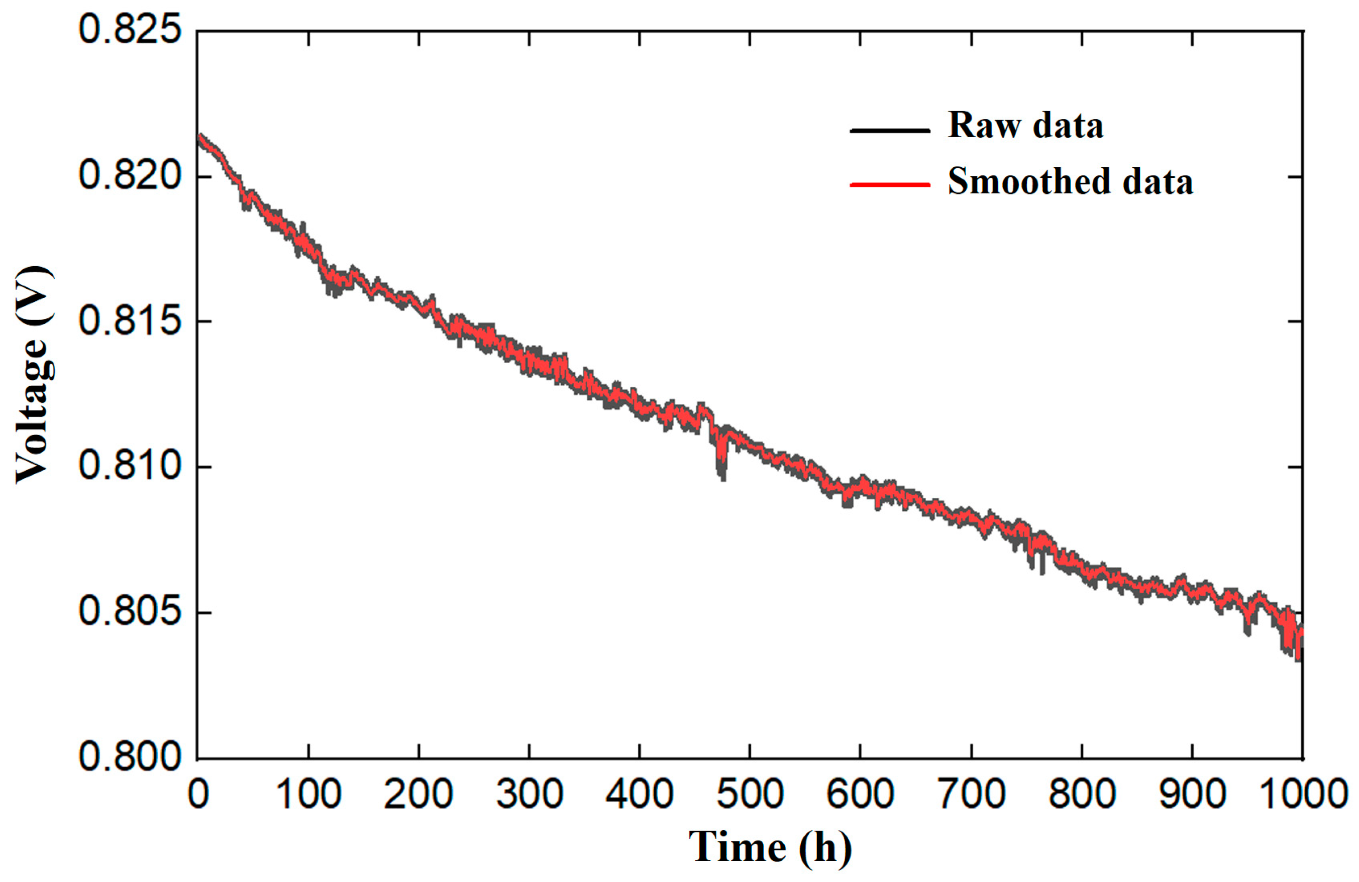
4.1. Experimental Raw Data Preprocessing

Inspired by the literature [29], the output voltage of the SOFC system is considered the time-aging indicator in the prognostics process. Since the experimental raw voltage data involve many noises and peaks, many measurement points may lead to heavy computational load (and are time consuming). Therefore, data preprocessing is highly required to improve the qualitative nature of original raw voltage data. We utilized the robust locally weighted scatterplot filtered approach (LOWESS) to smooth the raw measurement for the subsequent processing [32]. The filtered algorithm consists of weighted linear least squares and second-order polynomial models. By computing the window width weight of each data point in the span of the smooth, the original raw data with noises and peaks can be effectively filtered. The weight coefficients are given as follows:

$$\begin{gathered} w_i=\left\{\begin{array}{c}{\left(1-{\left(\frac{y_i-{\widehat{y}}_i}{6MAD}\right)}^2\right)}^2,\left|y_i-{\widehat{y}}_i\right|<6\mathrm{MAD}\\ 0, \left|y_i-{\widehat{y}}_i\right|\ge 6\mathrm{MAD}\end{array}\right\} \\ \mathrm{MAD}=\mathrm{median}\left(\left|y_i-{\widehat{y}}_i\right|\right) \end{gathered}$$

(12)

where $y_i$ and ${\widehat{y}}_i$ are real and fit data, respectively, $y_i-{\widehat{y}}_i$ denotes the residual of the i_th data point generated by regression smoothing procedures, and MAD is treated as the median absolute deviation of the residual. The spread-out of the residual is computed by median absolute deviation.

The original raw datum is reconstructed by LOWESS to improve the quality and still retain the characteristic phenomenon. To deal with the reconstructed data, the window width is one of the key parameters. When the filter window width is small, the smooth data are closer to the original values, leading to a meaningless smooth result. On the contrary, if the window width is large, minor weight variations in the short time duration might not be detected. Therefore in this work, we set the window width filter to 20. Figure 4 shows raw and smooth data of the SOFC voltage with the elapsed time. It can be seen that the original voltage data with noises and spikes are clearly smoothed, with a consistent trend, compared to the raw experimental data after preprocessing. The preprocessing of smoothed data not only reduce uncertainty, but also retain the main characteristic tendencies of the original raw data. The data set dimensions include gas flow rate, cell temperature, humidity, current, voltage, pressure, etc. The dimensionality difference among parameters between the input and output significantly cause data distortion. To further reduce the impact of substantial variable differences on the model performance, the original raw data must be standardized to extract the feature data into the interval [0, 1]. The standardized method is proposed by the following formula:

$$\acute{y}=\frac{y-y_{min}}{y_{max}-y_{min}}$$

(13)

where $\acute{y}$ is the standardized data, y is the original raw data, y_max is the maximum value of the original data, and y_min is the minimum value of original data.

4.2. Feature Extraction of Neural Network Structures

In the present study, the proposed methods for prognostics of the SOFC system performance were conducted by MATLAB, a trademark of MathWorks, Inc. (Natica, MA, USA) [33]. The optimal dynamic neural unit parameters of NNARX structures, such as hidden neural number (h_n), model output order (n_a), model input order (n_b), and the time delay (n_k), were computed by Taguchi orthogonal array methods. The parameters were selected by statistical analysis to compute the best performance of prediction. The detailed statement of the experimental analysis result is provided by a previous published paper [25].

For consistency, the parameter structures of relative repressors for NNARMAX and NNOE should be conducted under the same conditions as the NNARX model. The performance degradation predictions of the SOFC system, based on the NN structures with NNARX, NNARMAX, and NNOE models, were compared by evaluating their convergence accuracies with the normalized sum square error (NSSE). Every neuron network structure was conducted with a tangent-sigmoid activation function and the output layer with a linear transfer function for these three models.

Comparison results of different model type convergent iteration graphs in the learning phase are shown in Figure 5. It can be seen that, although the convergence rate of the NNARX model is slower than other model types, the number of stable convergence iterations is superior to others.

Table 2. The selected repressor parameters and analysis results of DNN models.

Dynamic Neural Unit
Model	Hidden Number (hn)	Output Order (na)	Input Order (nb)	Noise Order (nc)	Time Delay (nk)	NSSE
NNARX	10	5	5	None	1	1.32 × 10−10
NNARMAX	10	5	5	1	1	3.43 × 10−7
NNOE	10	5	5	None	1	6.56 × 10−5

lists the dynamic neural unit values and the analysis results of convergences accuracy for the proposed DNN model types based on NNARX, NNARMAX, and NNOE model structures. From the analysis results, the proposed DNN models have lower NSSE values, which indicate that the prediction model has high accuracy and can prove that the selected dynamic neural unit is acceptable.

4.3. Performance Evaluation Criteria

In order to compare the accuracy of long-term prediction degradation trend results, a series of evaluation criteria should be put forward. In this study, the symbols of the root mean square error (RMSE), and mean absolute error (MAE), were selected to test the prediction performance degradation trend reliability, and were used for quantitatively comparing the cumulative errors over the entire range of the proposed prognostics methods.

$$\mathrm{RMSE}=\sqrt{\frac{1}{\mathrm{N}}{\displaystyle \sum }_1^{\mathrm{N}}({\left(\mathrm{p}\left(\mathrm{t}\right)-\hat{\mathrm{p}}\left(\mathrm{t}\right)\right)}^2}$$

(14)

$$\mathrm{MAE}=\frac{1}{\mathrm{N}}{\displaystyle \sum }_1^{\mathrm{N}}\left|(\mathrm{p}\left(\mathrm{t}\right)-\hat{\mathrm{p}}\left(\mathrm{t}\right)\right|$$

(15)

where p(t) is the experimental measurement voltage value, $\hat{\mathrm{p}}\left(\mathrm{t}\right)$ is the model predicted voltage value, and N is the number of the measured voltage. The performance of the criteria index is “smaller is better”.

After that, the evaluation indexes—relative error (RE) and prediction accuracy (PA)—were used to evaluate the results of the RUL estimation between the actual RUL and predicted one. The relevant formula is calculated as follows:

$$\mathrm{RE}=\left|\frac{{\mathrm{RUL}}_{EoL\_actual}-{\mathrm{RUL}}_{EoL\_prognostic}}{{\mathrm{RUL}}_{EoL\_prognostic}}\right|\times 100\%$$

(16)

$$\mathrm{PA}=1-\mathrm{RE}$$

(17)

where EoL represents the end of life of system. RUL_{EoL_actual} indicates the actual RUL and RUL_{EoL_prognostic} denotes the predicted RUL. In regard to the performance index of PA—higher is more accurately.

5. Results and Discussion

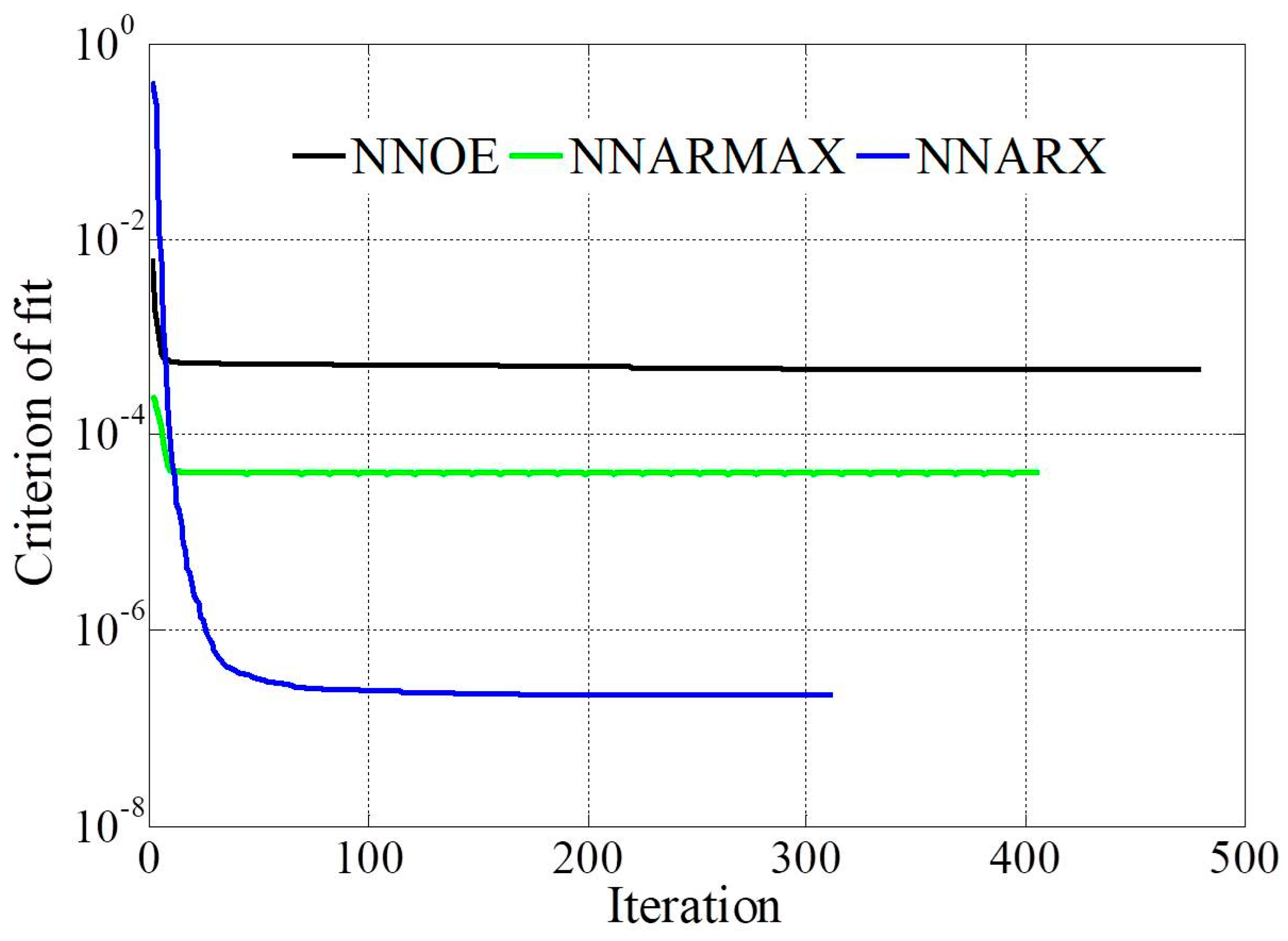
5.1. Comparison of Performance Degradation Prediction

The prognostics framework of the SOFC system includes two parts: learning phase and inference phase. Moreover, by evaluating the proposed prognostics method for the aging degradation trend prediction and RUL estimation of SOFC, the data set was divided into 50% for the learning phase and the remaining for the inference phase, because the arrangement can sufficiently capture the characteristics of the system and avoid overfitting during the prognostic processes [34]. The total data set duration of the SOFC long-term experiment was 1000 h. The time lengths of [0 h, 500 h] and [501 h, 1000 h] were selected as the learning phase and inference phase, respectively. A comparison among the degradation trend predicted results, namely NNARX, NNARMAX, and NNOE models, and experimental measurement data were made for variations of SOFC voltages over time, as shown in Figure 6. It is obvious that the degradation trend behavior of the SOFC system can be tracked by all three nonlinear NN models during the prognostics processes.

Comparison results on prediction accuracy between the learning phase and inference phase, within the statistic indices RMSE and MAE, are shown in Figure 7 and Figure 8, respectively. According to the performance criteria index in the prognostics processes, the results of the NNARX model have the lowest values. The best accuracies of RMSE (1.58 × 10⁻⁶) and MAE (9.3 × 10⁻⁷) were achieved by using the NNARX model with a small variation compared to the actual experimental data in the learning phase, and the values of RMSE and MAE of the inference phase were 1.86 × 10⁻⁶ and 9.4 × 10⁻⁷, respectively. For the NNARMAX model, the RMSE and MAE in the learning phase were 8.19 × 10⁻⁵ and 5.83 × 10⁻⁵, respectively, but increased to 1.23 × 10⁻⁴ and 8.05 × 10⁻⁵, respectively, in the inference phase. The worst accuracy was obtained by the NNOE model and the values of RMSE and MAE were 1.11 × 10⁻⁴ and 8.80 × 10⁻⁵, respectively, in the learning phase, and 3.40 × 10⁻³ and 3.02 × 10⁻³, respectively, in the inference phase. It can be concluded that the prediction of the degradation trend can be captured qualitatively by all three models in the learning phase. The comparison predictions of the learning phase and inference phase using NNARX, NNARMAX, and the NNOE models are further summarized in

Table 3. Comparison results of prediction for various nonlinear DNN models in the learning phase and inference phase.

	RMSE		MAE
Model	Learning Phase	Inference Phase	Learning Phase	Inference Phase
NNARX	1.58 × 10−6	1.86 × 10−6	9.30 × 10−7	9.44 × 10−7
NNARMAX	8.19 × 10−5	1.23 × 10−4	5.83 × 10−5	8.05 × 10−5
NNOE	1.11 × 10−4	3.40 × 10−3	8.80 × 10−5	3.02 × 10−3

.

On the soft computing theory of the nonlinear system, the NNARX model is defined as a parallel structure in a series, while the NNARMAX and NNOE model are parallel structures. It indicates the NNARMAX and NNOE model structures are constituted by output feedback estimation. However, the NNARX model structure is determined by the current output with the combination of past inputs and outputs. Hence, the computation form of NNARX is stable and the parameters are easy to evaluate without feedback. In contrast, the current output of the NNARMAX model is computed by the combination of previous inputs, outputs, and residuals. Thus, the parameter structure of residual regression is applied to compensate feedback for the stability during the computation process. Moreover, the NNOE model structure is based on past and present output values, leading to unstable computation and insufficient predictive ability easily. It demonstrates that the NNARX model prediction degradation trend ability is better than other NARMAX and NNOE models. Although the performance indexes of the NNOE model, i.e., RMSE and MAE, are higher than the other two models, the prediction degradation trend still has the same consistency with experimental data.

In order to verify the prediction accuracy of the proposed method, the prediction results are compared of open literature methods based on backpropagation (BP), support vector machine (SVM), and random forest (RF) [35], as shown in

Table 4. Comparison results of prediction accuracy with previous methods.

Method	RMSE	MAE
NNARX	$1.72\times {10}^{-6}$	$9.37\times {10}^{-7}$
NNARMAX	$1.02\times {10}^{-4}$	$6.94\times {10}^{-5}$
NNOE	$1.76\times {10}^{-3}$	$1.55\times {10}^{-3}$
Backpropagation (BP) [35]	0.0032	0.0769
Support vector machine (SVM) [35]	0.4492	0.2998
Random forest (RF) [35]	0.524	0.3598

. From the results shown, the average criteria of the proposed methods (learning phase and inference phase) are lower than other existing methods. Although the data lengths are different, the comparison results can still demonstrate the effectiveness of the proposed DNN models based on NNARX, NNARMAX, and NNOE.

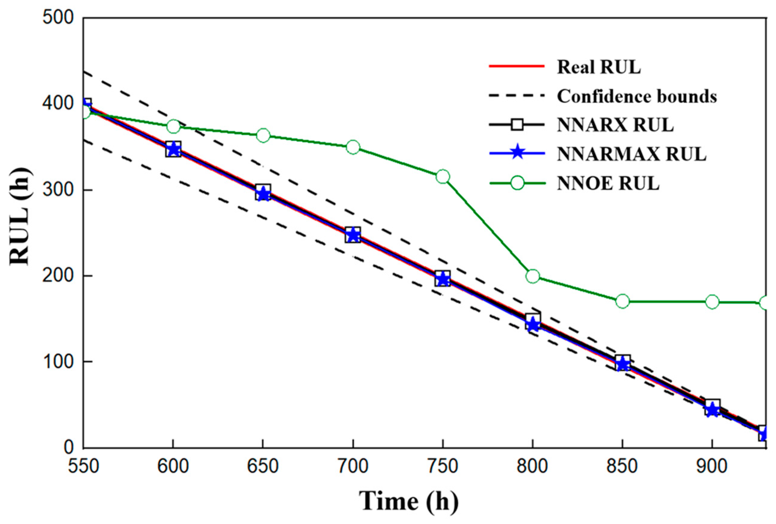
5.2. Remaining Useful Lifetime Inference

Based on the results of the proposed NN model structure obtained during the learning phase, the second half samples were used to estimate the RUL of the SOFC system. From the literature, the SOFC stack failures can be explained as the water vapor produced by the cathode, preventing the delivery capability of ambient air, or the compound produced by the anode, leading to the degradation of the SOFC system [36,37]. In order to protect the SOFC system and adopt timely mitigation actions, a critical threshold, a little higher than the failure threshold, should be defined in advance.

According to the failure definition in international standards [38], when the cell voltage declines more than 2% of the initial voltage, the fault of the SOFC stack is diagnosed, and the SOFC failure is considered to occur soon, requiring possible preventive maintenance [39]. When the prognostics time (T_p) starts at time T_p = 500 h for the inference phase, the estimation voltage is computed based on the parameters determined by the nonlinear neural network structures with NNARX, NNARMAX, and NNOE models in the learning phase. Therefore, the RUL denotes the time period between the T_p and end of life (EoL) in the inference phase.

As shown in Figure 6, the real measured voltage is indicated by the red line, while the estimated voltages, i.e., NNARX, NNARMAX, and NNOE, are denoted in the black, blue, and green lines, respectively. When the experimental output voltage value of the SOFC system decreases to 0.805 V, the corresponding RUL time is set as the EoL time T_EoL = 947.71 h, which indicates that the mitigation strategy is required against the failure. Since the inference time scale is set at 500–1000 h, the RUL is 447.71 h. From the RUL estimation results, all NNARX, NNARMAX, and NNOE can efficiently capture the degradation trend of the SOFC performance, attributed to the appropriate variable selection analysis of input parameters.

During the inference phase of the RUL estimation, the prognostic evolutions of the NNARX and NNARMAX models approach the critical threshold between 947.19 and 947.04 h, which is close to that of the measured value. The RUL times of NNARX and NNARMAX are 447.19 h and 447.04 h, respectively, which is lower than the real RUL value of 447.71 h. On the other hand, the predictive curve of the NNOE model can fit the experimental value well in the beginning of the prognostic period. However, it drops rapidly after T = 520 h and reaches the critical threshold of 805 V at T = 775.81 h.

Although the NNOE model has a deviation from the real values, its predicted tendency is still consistent with experimental data. It can be reasonably ascertained that all three models can be used as diagnostic methods for predicting the RUL. In

Table 5. Comparison analysis results of the proposed models.

Models	RUL_prognostic	AE	RE	PA
NNARX	447.19	0.52	0.12%	99.88%
NNARMAX	447.04	0.67	0.15%	99.85%
NNOE	275.81	171.9	38.40%	61.6%

, the RUL prediction errors among the estimated and actual values, absolute error (AE), and RE of the NNARX model are less than the NNARMAX and NNOE models at the inference phase, leading to a higher prediction accuracy. It was also found that these AE and RE values of the NNOE model are relatively higher than those of the NNARX and NNARMAX models.

For further uncertainty analysis of the RUL estimation, the inference was carried out every 50 h after T = 500 h within the 1 $\pm$ 0.05% confidence intervals with the upper and lower boundaries, as shown by black dash lines in Figure 9. The results of the RUL estimation show that both NNARX and NNARMAX models agree very well with the actual RUL values and always fall into the confidence intervals.

By comparison with the real RUL, the RUL estimation of the NNOE model presents an overestimation in the range considered after T = 600 h and begins beyond the upper boundary of the confidence interval after T = 650 h. Although the NNOE model can correctly capture the fuel cell degradation trend in the learning stage, it shows the weak generalization ability in the RUL inference phase. This is attributed to the fact that the parameter structure of the NNOE model belongs to the recursive regression method, leading to the difficulty of the model parameter estimation.

Based on the present results, the prognostic of the NNARX model not only depict the trend of the voltage degradation, but is also appropriate in quantitative accuracy for the RUL prediction.

6. Conclusions

This paper presents DNN model structures based on NNARX, NNARMAX, and NNOE models, to predict the performance degradation and the RUL estimation for the SOFC system. The proposed method was conducted based on the SOFC long-term degradation test. The results indicate that the proposed model, based on the NNARX model, has the best prognostic performance. Based on the present results, the main contribution might be summarized as follows:

(1)

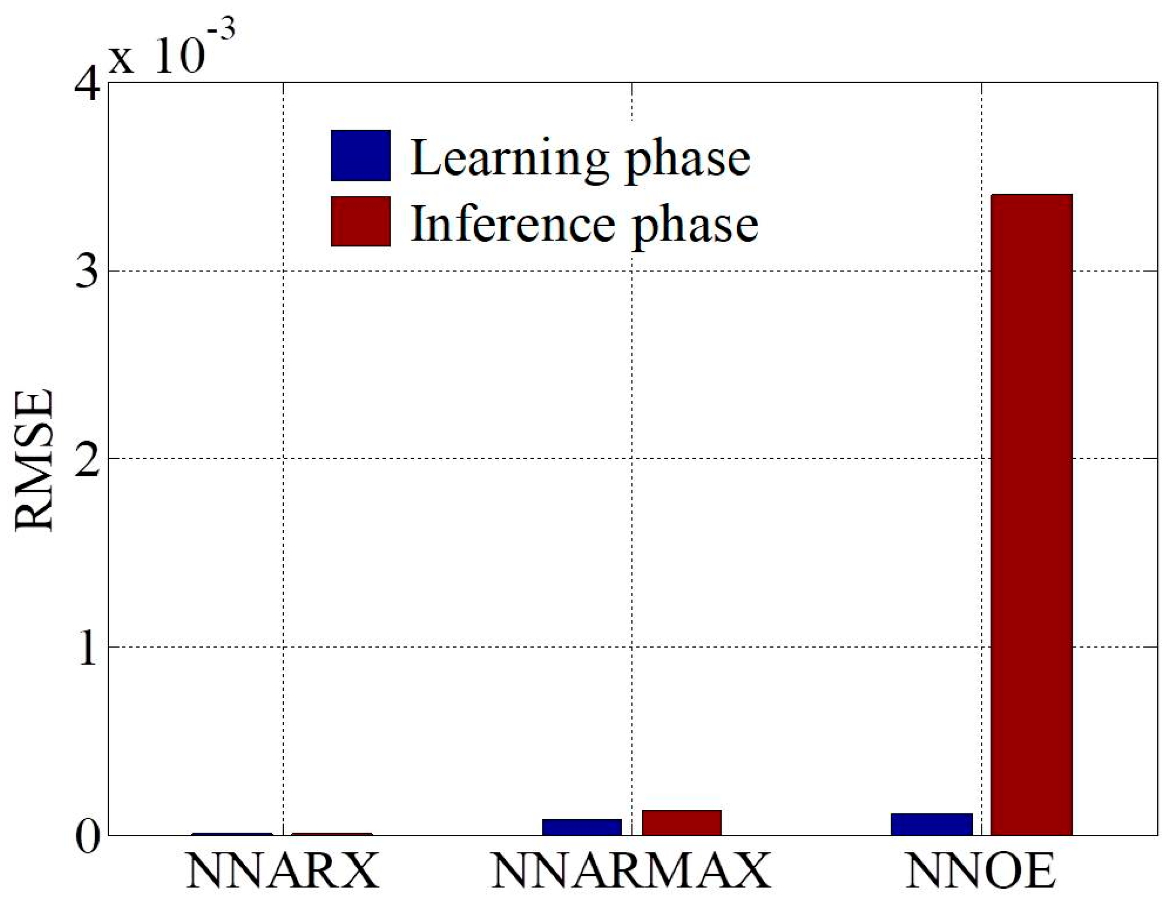
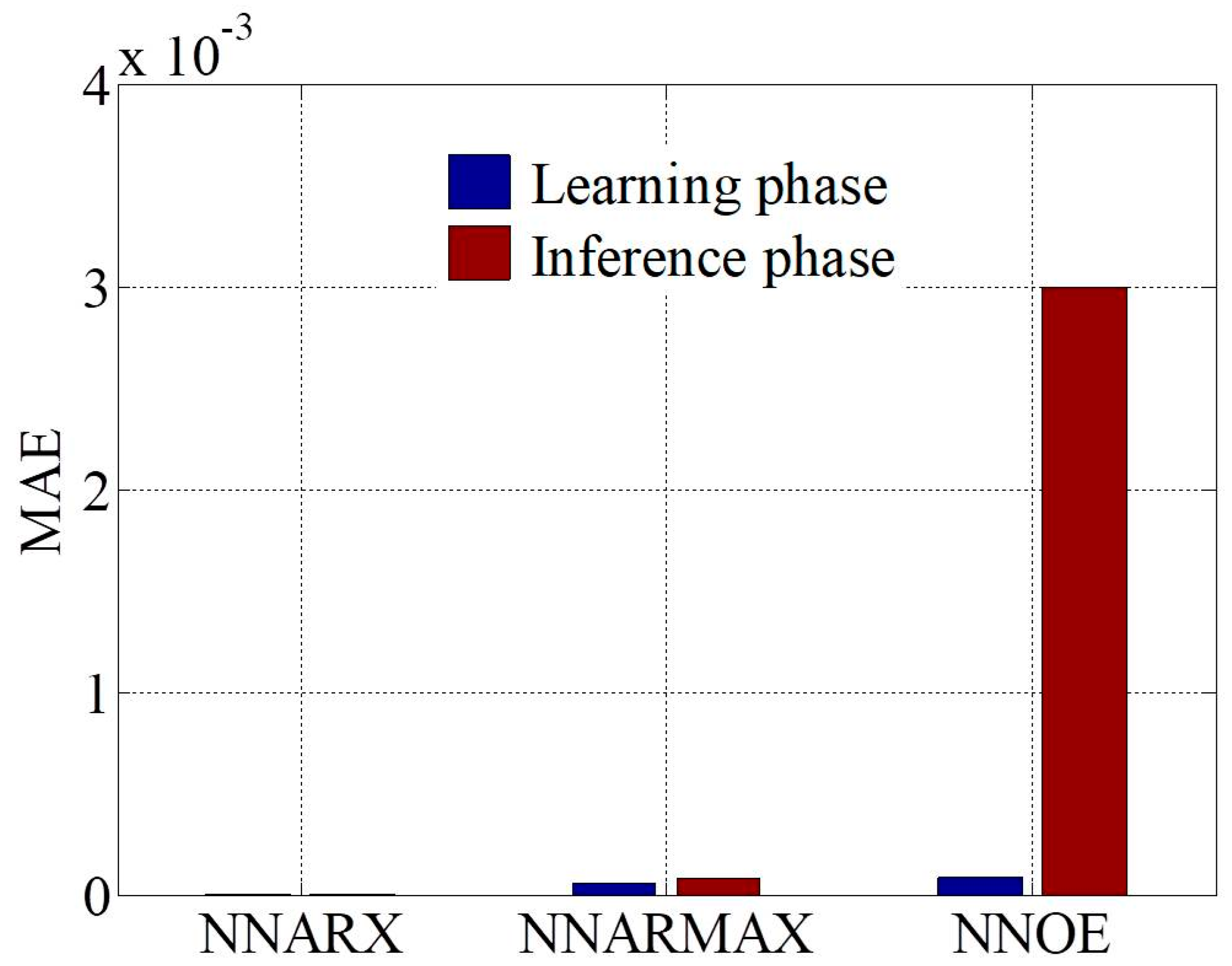
In the learning phase, the proposed models can efficiently capture the degradation trend of the SOFC performance. During the inference phase, the NNARX model provides higher (and more accurate) prognostic performances than the other NNARMAX and NNOE models.

(2)

In the DNN model structures, the NNARX model has low values of RMSE and MAE due to parallel structure in a series. Although both NNARMAX and NNOE are parallel structures, the computation form of the NNARX model is stable, leading to better prognostics accuracy than the NNOE model.

(3)

The results of the RUL estimation demonstrate that both NNARX and NNARMAX models not only agree very well with the actual RUL values, but also “fall into” the confidence intervals. Although the NNOE model has a deviation from the real RUL values, its predicted tendency is still qualitatively consistent with experimental data.

(4)

Comparing the results with previous prognostic methods from the open literature, the proposed methods of the DNN models present better performances.

References

1. Saebea, D.; Authayanun, S.; Patcharavorachot, Y. Performance analysis of direct steam reforming of methane in SOFC with SDC-based electrolyte. Energy Rep. 2020, 6, 391–396. [Google Scholar] [CrossRef]
2. Xu, H.; Ma, J.; Tan, P.; Chen, B.; Wu, Z.; Zhang, Y.; Wang, H.; Xuan, J.; Ni, M. Towards online optimization of solid oxide fuel cell performance: Combining deep learning with multi-physics simulation. Energy AI 2020, 1, 1–11. [Google Scholar] [CrossRef]
3. Lanzini, A.; Ferrero, D.; Papurello, D.; Santarelli, M. Reporting Degradation from Different Fuel Contaminants in Ni-anode SOFCs. Fuel Cells 2017, 17, 423–433. [Google Scholar] [CrossRef]
4. Faro, M.L.; Antonucci, V.; Antonucci, P.; Aricò, A. Fuel flexibility: A key challenge for SOFC technology. Fuel 2012, 102, 554–559. [Google Scholar] [CrossRef]
5. Zhang, L.; Lin, J.; Liu, B.; Zhang, Z.; Yan, X.; Wei, M. A review on deep learning applications in prognostics and health management. IEEE Access 2019, 7, 162415–162438. [Google Scholar] [CrossRef]
6. Chen, K.; Laghrouche, S.; Djerdir, A. Proton exchange membrane fuel cell prognostics using genetic algorithm and extreme learning machine. Fuel Cells 2020, 20, 263–271. [Google Scholar] [CrossRef]
7. Lecoeuche, S.; Lalot, S. Prediction of the daily performance of solar collectors. Int. Commun. Heat Mass Transf. 2005, 32, 603–611. [Google Scholar] [CrossRef]
8. Perera, A.T.D.; Wickramasinghe, P.; Nik, V.M.; Scartezzini, J.L. Introducing reinforcement learning to the energy system design process. Appl. Energy 2020, 262, 114580. [Google Scholar] [CrossRef]
9. Huang, Q.A.; Hui, R.; Wang, B.; Zhang, J. A review of AC impedance modeling and validation in SOFC diagnosis. Electrochim. Acta 2007, 52, 8144–8164. [Google Scholar] [CrossRef]
10. Kakac, S.; Pramuanjaroenkij, A.; Zhou, X.Y. A review of numerical modeling of solid oxide fuel cells. Int. J. Hydrogen Energy 2007, 32, 761–786. [Google Scholar] [CrossRef]
11. Hajimolana, S.A.; Hussain, M.A.; Daud, W.A.W.; Soroush, M.; Shamiri, A. Mathematical modeling of solid oxide fuel cells: A review. Renew. Sustain. Energy Rev. 2011, 15, 1893–1917. [Google Scholar] [CrossRef]
12. Seborg, D.E.; Mellichamp, D.A.; Edgar, T.F.; Doyle, F.J., III. Process Dynamics and Control; John Wiley & Sons: Hoboken, NJ, USA, 2010. [Google Scholar]
13. Wang, K.; Hissel, C.; Péra, M.C.; Steiner, N.; Marra, D.; Sorrentino, M.; Pianese, C.; Monteverde, M.; Cardone, P.; Saarinen, J. A review on solid oxide fuel cell models. Int. J. Hydrogen Energy 2011, 36, 7212–7228. [Google Scholar] [CrossRef]
14. Song, C.; Lee, S.; Gu, B.; Chang, I.; Cho, G.Y.; Baek, F.D.; Cha, S.W. A Study of Anode-Supported Solid Oxide Fuel Cell Modeling and Optimization Using Neural Network and Multi-Armed Bandit Algorithm. Energies 2020, 13, 1621. [Google Scholar] [CrossRef] [Green Version]
15. Cheng, S.J.; Liu, J.J. Nonlinear modeling and identification of proton exchange membrane fuel cell (PEMFC). Int. J. Hydrogen Energy 2015, 40, 9452–9461. [Google Scholar] [CrossRef]
16. He, Y.J.; Ma, Z.F. A Data-Driven Gaussian Process Regression Model for Two-Chamber Microbial Fuel Cells. Fuel Cells 2016, 16, 365–376. [Google Scholar] [CrossRef]
17. Wang, X.; Balakrishnan, N.; Guo, B. Residual life estimation based on a generalized Wiener degradation process. Reliab. Eng. Syst. Saf. 2014, 124, 13–23. [Google Scholar] [CrossRef]
18. Wu, X.; Ye, Q. Fault diagnosis and prognostic of solid oxide fuel cells. J. Power Sources 2016, 321, 47–56. [Google Scholar] [CrossRef]
19. Bressel, M.; Hilairet, M.; Hissel, D.; Bouamama, B.Q. Extended Kalman filter for prognostic of proton exchange membrane fuel cell. Appl. Energy 2016, 164, 220–227. [Google Scholar] [CrossRef]
20. Fathy, A.; Rezk, H.; Ramadan, H.S.M. Recent moth-flame optimizer for enhanced solid oxide fuel cell output power via optimal parameters extraction process. Energy 2020, 207, 118326. [Google Scholar] [CrossRef]
21. Milewski, J.; Świrski, K. Modelling the SOFC behaviours by artificial neural network. Int. J. Hydrogen Energy 2009, 34, 5546–5553. [Google Scholar] [CrossRef]
22. Bai, H.; Liu, C.; Breaz, E.; Gao, F. Artificial neural network aided real-time simulation of electric traction system. Energy AI 2020, 1, 100010. [Google Scholar] [CrossRef]
23. Sinha, N.K.; Gupta, M.M.; Rao, D.H. Dynamic Neural Networks: An Overview. In Proceedings of the IEEE International Conference on Industrial Technology 2000, Goa, India, 19–22 January 2000; pp. 491–495. [Google Scholar]
24. Lang, K.J.; Waibel, A.H.; Hinton, G.E. A Time-Delay Neural Network Architecture from Isolated Word Recognition. Neural Netw. 1990, 3, 23–44. [Google Scholar] [CrossRef]
25. Gupta, M.M.; Rao, D.H. Neural Units with Applications to the Control of Unknown Nonlinear Systems. J. Intell. Fuzzy Syst. 1993, 1, 73–92. [Google Scholar] [CrossRef]
26. Lee, D.; Lin, J.K.; Tsai, C.H.; Wu, S.H.; Cheng, Y.N.; Lee, R.Y. Analysis of Long-Term and Thermal Cycling Tests for a Commercial Solid Oxide Fuel Cell. J. Electrochem. Energy 2017, 14, 041002. [Google Scholar] [CrossRef]
27. Tsai, C.H.; Hwang, C.S.; Chang, C.L.; Yang, S.F.; Cheng, S.W.; Shie, Z.Y.C.; Hwang, T.J.; Lee, R.Y. Performance and long term durability of metal-supported solid oxide fuel cells. J. Ceram. Soc. Jpn. 2015, 123, 205–212. [Google Scholar] [CrossRef] [Green Version]
28. Cheng, Y.N.; Cheng, S.W.; Lee, R.Y. The Comparisons of Electrical Performance and Impedance Spectrum for Two Commercial Cells. J. Fuel Cell Sci. Technol. 2014, 11, 051002–051006. [Google Scholar] [CrossRef]
29. Jouin, M.; Bressel, M.; Morando, S.; Gouriveau, R.; Hissel, G.; Péra, M.C.; Zerhouni, N.; Jemei, S.; Hilairet, M.; Bouamama, B.O. Estimating the end-of-life of PEM fuel cells: Guidelines and metrics. Appl. Energy 2016, 177, 87–97. [Google Scholar] [CrossRef] [Green Version]
30. Lyu, J.; Zhang, J. BP neural network prediction model for suicide attempt among Chinese rural residents. J. Affect. Disord. 2019, 246, 465–473. [Google Scholar] [CrossRef] [PubMed]
31. Cheng, S.J.; Lin, J.K. Performance Prediction Model of Solid Oxide Fuel Cell System Based on Neural Network Autoregressive with External Input Method. Processes 2020, 8, 828. [Google Scholar] [CrossRef]
32. Kimmel, R.K.; Booth, D.E.; Booth, S.E. The analysis of outlying data points by robust Locally Weighted Scatter Plot Smooth: A model for the identification of problem banks. Int. J. Oper. Res. 2010, 7, 1–15. [Google Scholar] [CrossRef]
33. Beale, M.H.; Hagan, M.T.; Demuth, H.B. Users’ Guide for the Neural Network Toolbox for MATLAB; The Mathworks: Natica, MA, USA, 2017. [Google Scholar]
34. Liu, H.; Chen, J.; Hou, M.; Shao, Z.; Su, H. Data-based short-term prognostics for proton exchange membrane fuel cells. Int. J. Hydrogen Energy 2017, 42, 20791–20808. [Google Scholar] [CrossRef]
35. Song, S.; Xiong, X.; Wu, X.; Xue, X. Modeling the SOFC by BP neural network algorithm Modeling the SOFC by BP neural network algorithm. Int. J. Hydrogen Energy 2021, 46, 20065–20071. [Google Scholar] [CrossRef]
36. Nakajo, A.; Mueller, F.; Brouwer, J.; Favrat, D. Mechanical reliability and durability of SOFC stacks. Part II: Modelling of mechanical failures during ageing and cycling. Int. J. Hydrogen Energy 2012, 37, 9269–9286. [Google Scholar] [CrossRef] [Green Version]
37. Colombo, K.W.E.; Kharton, V.V.; Berto, F.; Paltrinieri, N. Mathematical modeling and simulation of hydrogen-fueled solid oxide fuel cell system for micro-grid applications-Effect of failure and degradation on transient performance. Energy 2020, 202, 117752. [Google Scholar] [CrossRef]
38. I.S. Organization. Condition Monitoring and Diagnostics of Machinery-Prognostics—Part 1: General Guidelines; Technical Report ISO 13381-1; ISO: Geneva, Switzerland, 2004; pp. 1–20. [Google Scholar]
39. Mosallam, A.; Medjaher, K.; Zerhouni, N. Data-driven prognostic method based on Bayesian approaches for direct remaining useful life prediction. J. Intell. Manuf. 2016, 27, 1037–1048. [Google Scholar] [CrossRef]
Figure 1. The schematic device of the SOFC test [26].
Energies 14 05841 g001
Figure 2. The basic architecture of DNN model [24].
Energies 14 05841 g002
Figure 3. Flow chat of the DNN model for SOFC system prognostic.
Energies 14 05841 g003
Figure 4. Raw and smooth long-term degradation data of the SOFC voltage.
Energies 14 05841 g004
Figure 5. Comparison results of different DNN models convergent iteration.
Energies 14 05841 g005
Figure 6. Comparison results of the SOFC degradation trend prediction and RUL estimation by different DNN models.
Energies 14 05841 g006
Figure 7. RMSE of the degradation prediction in the learning phase and inference phase.
Energies 14 05841 g007
Figure 8. MAE of the degradation prediction in the learning phase and inference phase.
Energies 14 05841 g008
Figure 9. Uncertainty analysis of RUL estimation within different models.
Energies 14 05841 g009