Numerical Simulation of Heat Transport Problems in Porous Media Coupled with Water Flow Using the Network Method

Abstract

In the present work, a network model for the numerical resolution of the heat transport problem in porous media coupled with a water flow is presented. Starting from the governing equations, both for 1D and 2D geometries, an equivalent electrical circuit is obtained after their spatial discretization, so that each term or addend of the differential equation is represented by an electrical device: voltage source, capacitor, resistor or voltage-controlled current source. To make this possible, it is necessary to establish an analogy between the real physical variables of the problem and the electrical ones, that is: temperature of the medium and voltage at the nodes of the network model. The resolution of the electrical circuit, by means of the different circuit resolution codes available today, provides, in a fast, simple and precise way, the exact solution of the temperature field in the medium, which is usually represented by abaci with temperature-depth profiles. At the end of the article, a series of applications allow, on the one hand, to verify the precision of the numerical tool by comparison with existing analytical solutions and, on the other, to show the power of calculation and representation of solutions of the network models presented, both for problems in 1D domains, typical of scenarios with vertical flows, and for 2D scenarios with regional flow.

1. Introduction

The topic of heat transport coupled to water flow in porous media has aroused great interest among researchers in recent decades [1,2], finding in the literature a great variety of temperature-depth profiles, both for regional [3,4] and exclusively vertical flows [5,6] and for a wide variety of cases in the soil surface temperature condition [7,8,9,10,11]. The first advances in this discipline, whose processes are governed by coupled, non-linear PDEs derived from momentum, mass and energy conservation laws, date from the middle of the 20th century [12,13,14]. The patterns of solutions to this complex phenomenon are fundamental in many fields of engineering, such as the exploitation of geothermal energy extraction systems [15,16], saltwater intrusion [17], underground spread of pollutants [18] and petroleum engineering [19], among others.

In this research, the study of the heat transport problem partially coupled to a constant velocity field (either solved or previously known) corresponds to a linear problem, except for the surface boundary condition when it is a time-dependent function. The harmonic temperature conditions on the soil surface (which are the usual ones) give rise to a heat transport problem that is coupled with the movement of the fluid. These continuously changing conditions, although seasonally repetitive (day-night cycle; winter-summer cycle) determine equally changing temperature-depth profiles, with a certain inertia that is determined by the thermal parameters of the ground (conductivity and specific heat). Despite the changing conditions on the soil surface, it is possible to speak of stationary temperature-depth profiles, both on a daily and annual scale.

Within the great variety of numerical techniques that exist for solving these types of problems, it is worth highlighting the network simulation method [20], a finite volume numerical tool that allows studying any process that can be defined by means of a mathematical model that is composed of a set of differential equations. The method has two phases: (i) the elaboration of a network model (electrical circuit equivalent to the process) and (ii) the simulation of the problem (obtaining the results of the network model) by means of a suitable program that allows the resolution of electrical circuits [21,22]. Recently, this technique has been successfully used in the simulation of a wide variety of problems in different fields of engineering, such as electrochemistry [23,24], elasticity [25], heat transfer [26] and tribology [27], providing accurate solutions in all cases. Its versatility is so high that, provided the appropriate equivalences are established (geometric, of the model and its variables of interest), it could be applied in other fields of knowledge such as neural networks [28] or geometric modeling [29,30,31,32].

The network method, whose application must follow a series of formal steps that require simple programming rules, makes use of the powerful calculation algorithms that reside in the electrical circuit simulation codes, providing the exact solution of the problem with relatively small grid meshes [33]. It is, therefore, a reliable, easy-to-use and computationally fast numerical tool which, compared to other traditional finite-differences or finite-volumes methods, stands out for its simplicity in the design and in the elaboration of the model, in addition to the fact that its execution can be carried out using free access software [22].

It is important to highlight that with the network method it would be possible to model other problems similar to the one presented here and that have been recently studied by other authors. Thus, Koch et al. [34] present a very similar network model that includes the possibility of considering different fluid and solid phase temperatures. However, this situation of thermal non-equilibrium at the local level is typical of phenomena associated with chemical reactions, evaporation or heat/cold injections (among others) which do not occur in the groundwater flow scenarios that we address in this work. On the other hand, Koch et al. [34] use an integral approximation procedure, a different numerical technique than the one used here. In another recent work, Matias et al. [35] address porous media that change over time due to swelling and erosion processes. These phenomena end up modifying the permeability of the soil, which would lead to changes in the fluid velocity in those scenarios governed by hydraulic potentials (in the scenarios studied here, it is the fluid velocity itself that governs the problem).

In this article, starting from the governing equations of the heat transport problem partially coupled to a known and constant velocity field (with vertical or horizontal direction), the design of a network model that will allow the resolution of this type of problem, both in 1D and 2D rectangular geometries, is presented. Subsequently, and after verifying the results obtained with our tool with the existing solutions in the reference literature [7,8,9,10], a series of selected applications (both for regional flow and exclusively vertical upflow) will be simulated in which different functions (dependent on time) will be assumed for the boundary condition of the soil surface temperature, obtaining the temperature-depth profiles once the stationary situation has been reached.

2. Mathematical Model

In this section, the equations and boundary conditions that govern different scenarios that address the problem of heat transport coupled to a water flow will be presented.

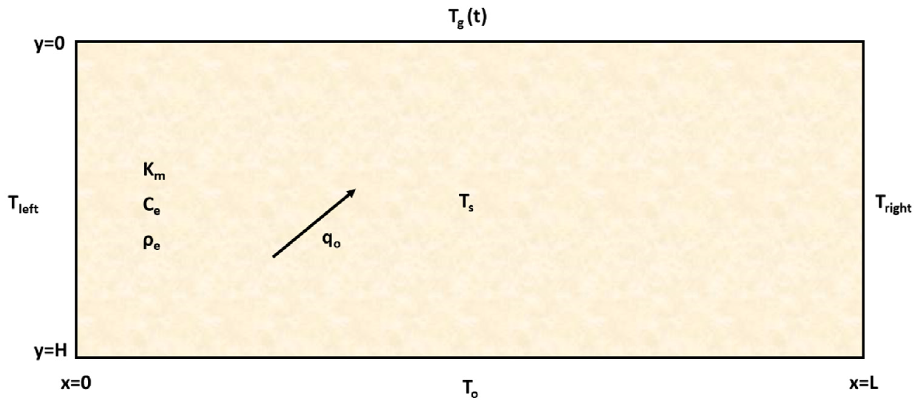
The physical model of the problem is that of a 2D rectangular geometry scenario that represents a fully saturated porous medium in which fluid flow and heat processes take place in such a way that the latter is coupled to the water flow (for vertical flow it will be enough to consider a one-dimensional domain). That is, the solution to the thermal problem depends on and is coupled to the solution of the mechanical problem.

The mechanical problem concerns the velocity field of water, which, for the purposes of this paper, will be uniform. That is, the water velocity will always be constant both in modulus, direction and sense, Equation (1). This consideration, although at first it seems quite strong, in certain groundwater flow scenarios it can be considered without committing major errors, as occurs in different real cases such as the discharge of an aquifer to the bottom of the sea or a lake (where the flow is exclusively vertical and it is usual for the velocity to be constant for long periods of time) or in regional (horizontal) flows [36], where it is also common to find large areas of aquifers with constant average velocities. On the other hand, the fact of knowing the velocity field (since it is imposed) makes the influence of viscosity (which is affected by temperature) negligible (fluid viscosity would affect velocities in those scenarios that were governed by hydraulic potential, but this is not the case with the problems discussed in this paper).

On the other hand, the thermal problem refers to the temperature field at each point of the porous medium, and is defined by the set of Equations (2)–(6) [1,2,3].

The mathematical model, according to the nomenclature of Figure 1, is as follows:

$$\mathrm{v}\left(\mathrm{x},\mathrm{y},\mathrm{t}\right)={ \mathrm{q}}_0$$

(1)

$$\left({\mathsf{\rho }}_{\mathrm{e}}{\mathrm{c}}_{\mathrm{e}}\right)\frac{\partial \mathrm{T}}{\partial \mathrm{t}}-{\mathrm{k}}_{\mathrm{m}}{\nabla }^2\left(\mathrm{T}\right)+{\mathsf{\rho }}_{\mathrm{w}}{\mathrm{c}}_{\mathrm{w}}{\mathrm{q}}_0\nabla \left(\mathrm{T}\right)=0$$

(2)

$${\mathrm{T}}_{\left(\mathrm{x},\mathrm{y}=\mathrm{H},\mathrm{t}\right)}={\mathrm{T}}_{\mathrm{o}}$$

(3)

$${\mathrm{T}}_{\left(\mathrm{x}=0,\mathrm{y},\mathrm{t}\right)}={\mathrm{T}}_{\mathrm{left}} \mathrm{and} {\mathrm{T}}_{\left(\mathrm{x}=\mathrm{L},\mathrm{y},\mathrm{t}\right)}={\mathrm{T}}_{\mathrm{right}}$$

(4)

$${\mathrm{T}}_{\left(\mathrm{x}, \mathrm{y}=0, \mathrm{t}\right)}={\mathrm{T}}_{\mathrm{g}}$$

(5)

$$\left\{\begin{array}{c}{\mathrm{T}}_{\left(\mathrm{x}, \mathrm{y}=0, \mathrm{t}\right)}={\mathrm{T}}_1 (0\le \mathrm{t}<{\mathrm{t}}_1)\\ {\mathrm{T}}_{\left(\mathrm{x}, \mathrm{y}=0, \mathrm{t}\right)}={\mathrm{T}}_2 \left({\mathrm{t}}_1\le {\mathrm{t}}_2\right)\end{array}\right\}$$

(6)

$${\mathrm{T}}_{\left(\mathrm{x}, \mathrm{y}=0, \mathrm{t}\right)}={\mathrm{T}}_{\mathrm{m}}+{\mathrm{T}}_{\sin }\sin \left(\frac{2\mathsf{\pi }}{\mathrm{P}}\mathrm{t}\right)$$

(7)

$${\mathrm{T}}_{\left(\mathrm{x},\mathrm{y},\mathrm{t}=0\right)}={\mathrm{T}}_{\mathrm{s}}$$

(8)

where Equation (2) represents the balance of heat transport in the medium (governing equation particularized to the case of constant water velocity). Equation (3) represents a constant temperature condition (or Dirichlet condition) at the bottom of the domain, also called the first-class condition, while Equation (4) represents the same type of condition but in the lateral boundaries of the domain. Equations (5)–(7) define the temperature condition on the ground surface in the form of a constant value, a step function or a sinusoidal, respectively. L and H are the dimensions of the rectangular domain. Finally, Equation (8) represents the initial condition defined by the initial temperature in the entire soil domain.

Regarding the temperature conditions on the soil surface, Equations (5)–(7), it is important to note that, in principle, the only feasible boundary condition on this contour is the sinusoidal temperature distribution, Equation (7), equivalent to 24 h temperature variation for day and night. However, in this work, the conditions of constant (Equation (5)) and stepped (Equation (6)) temperature have also been included, for various reasons. The first one is to illustrate that with the network method it is very easy to implement any boundary condition. In fact, in future research we plan to work with other surface temperature functions (even with tabulated data) whose implementation in the network model is just as simple. On the other hand, the constant temperature condition can sometimes serve as a simplification to consider an average daily temperature, although it could also refer to a monthly or annual average. For its part, the stepped temperature condition could be assimilated to a simplification similar to the previous one, but instead of having a single daily average temperature, there are two (an average maximum temperature for the day and an average minimum temperature for the night).

2.1. Mathematical Model for Vertical Flow

The exclusively vertical flow of water in porous aquifers is a fairly common situation to find in practice [37]. Thus, for example, this type of flow occurs in situations such as the discharge of a river into an aquifer [38], two aquifers separated by an aquitard [39] or in those cases in which an aquifer discharges directly onto the bottom of the sea or a lake [2].

The governing Equation (2) becomes, for one-dimensional vertical flow of an incompressible fluid through homogeneous porous media, as follows:

$${\mathsf{\rho }}_{\mathrm{e}}{\mathrm{c}}_{\mathrm{e}}\frac{\partial \mathrm{T}}{\partial \mathrm{t}}={ \mathrm{k}}_{\mathrm{m}}\frac{{\partial }^2\mathrm{T}}{\partial {\mathrm{y}}^2}-{\mathsf{\rho }}_{\mathrm{w}}{\mathrm{c}}_{\mathrm{w}}{\mathrm{q}}_{\mathrm{o},\mathrm{y}}\frac{\partial \mathrm{T}}{\partial \mathrm{y}}$$

(9)

On the other hand, depending on the boundary and initial conditions adopted, three variants of the problem with exclusive vertical flow are defined, governed by Equation (9).

2.1.1. Constant Surface Temperature

It is a scenario where the temperature of the ground surface (${\mathrm{T}}_{\mathrm{g}}$) remains constant throughout the time, being different from the initial temperature of the soil mass (${\mathrm{T}}_{\mathrm{s}}$). It is also necessary to set a temperature at the bottom of the domain as a boundary condition (${\mathrm{T}}_{\mathrm{o}}$).

Table 1. Boundary and initial thermal conditions for constant surface temperature and vertical flow scenario.

Parameter	Value	Units
${\mathrm{T}}_{\mathrm{s}}$	8	°C
${\mathrm{T}}_{\mathrm{g}}$	22.35	°C
${\mathrm{T}}_{\mathrm{o}}$	8	°C

shows the values that these boundary and initial thermal conditions, Equations (3), (5) and (8), will take, for this case of vertical water flow and constant temperature on the ground surface, in the later applications section.

2.1.2. Stepped Surface Temperature

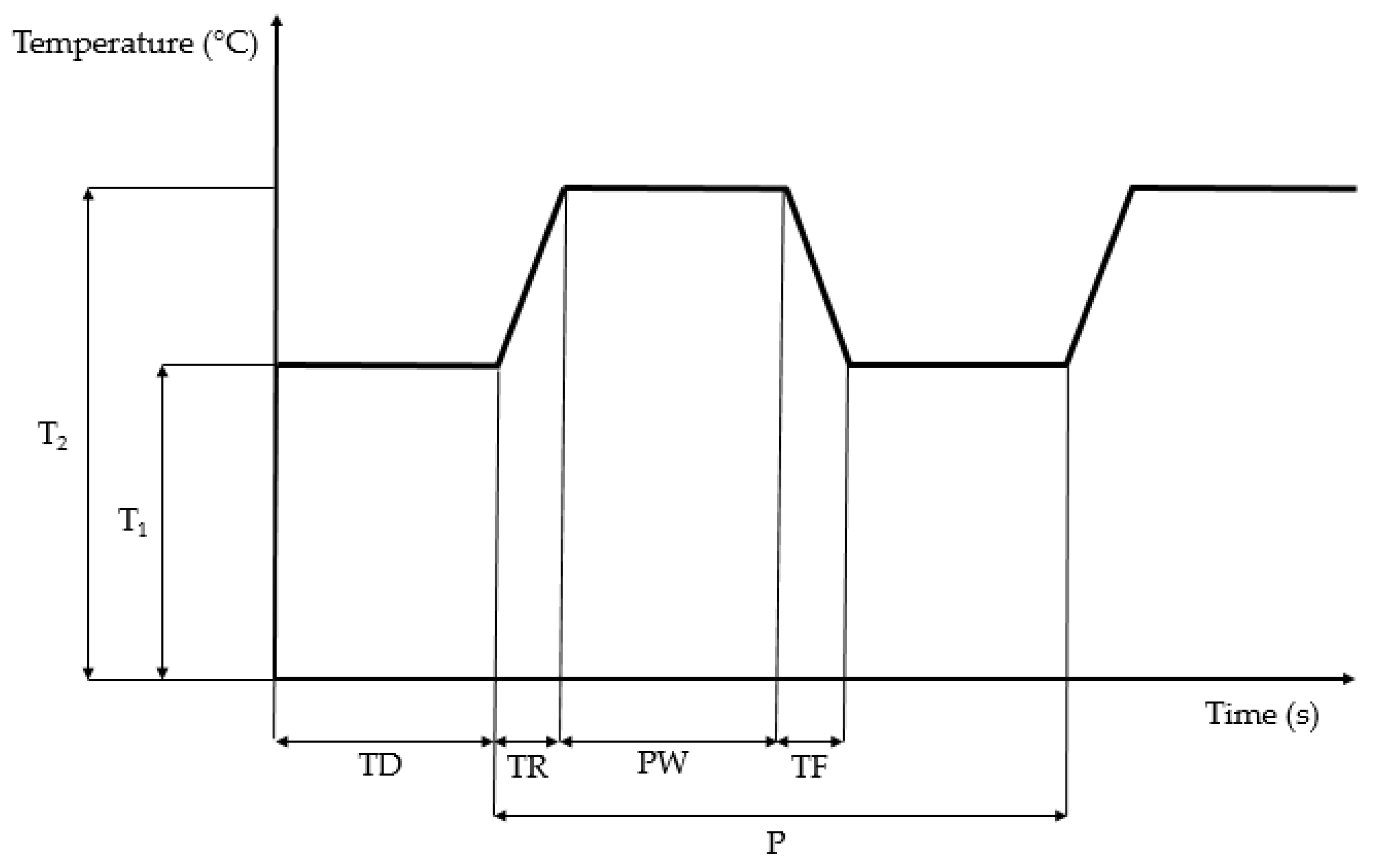
In this scenario, the surface temperature varies alternately between two values (simulating a period with a colder surface temperature, and a warmer one). To do this, it is necessary to define a stepped temperature function, Figure 2, which will be imposed as a boundary condition on the ground surface.

Table 2. Boundary and initial thermal conditions for stepped surface temperature and vertical flow scenario.

Parameter	Value	Units
${\mathrm{T}}_{\mathrm{s}}$	1	°C
${\mathrm{T}}_1$	0	°C
${\mathrm{T}}_2$	2	°C
${\mathrm{T}}_{\mathrm{D}}$	39,600	s
${\mathrm{T}}_{\mathrm{R}}$	3600	s
${\mathrm{T}}_{\mathrm{F}}$	3600	s
${\mathrm{P}}_{\mathrm{W}}$	39,600	s
$\mathrm{P}$	86,400	s
${\mathrm{T}}_{\mathrm{o}}$	(T2+T1)/2 = 1	°C

summarizes the boundary and initial thermal conditions, Equations (3), (6) and (8), for the case of vertical flow of water with stepped variation of the temperature on the ground surface that will be shown in the applications section.

2.1.3. Sinusoidal Surface Temperature

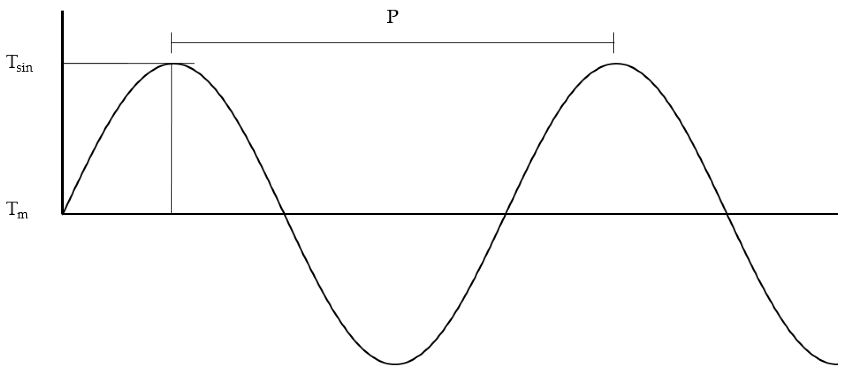
This time, the surface temperature varies following a sinusoidal function (simulating what can be, in certain situations, the temperature fluctuation throughout a day). On this occasion, a sinusoidal function will be imposed as a boundary condition on the ground surface, Figure 3.

Table 3. Boundary and initial thermal conditions for sinusoidal surface temperature and vertical flow scenario.

Parameter	Value	Units
${\mathrm{T}}_{\mathrm{s}}$	1	°C
${\mathrm{T}}_{\mathrm{m}}$	1	°C
${\mathrm{T}}_{\sin }$	1	°C
$\mathrm{P}$	86,400	s
${\mathrm{T}}_{\mathrm{o}}$	Tm = 1	°C

summarizes the boundary and initial thermal conditions, Equations (3), (7) and (8), for the case of vertical flow of water with sinusoidal temperature on the ground surface that will be numerically solved in the applications section.

2.2. Mathematical Model for Regional Flow

In hydrogeology, a regional flow is commonly called that whose movement of water is exclusively horizontal [3,4]. This type of water movement is typically found in underground hydrology, especially in aquifer extensions that are relatively far from the discharge area [40].

As described in [41], the general equation that describes the simultaneous flow of fluid and heat in the ground [37] is:

$${\mathrm{k}}_{\mathrm{m}}\left(\frac{{\partial }^2\mathrm{T}}{\partial {\mathrm{x}}^2}+\frac{{\partial }^2\mathrm{T}}{\partial {\mathrm{y}}^2}+\frac{{\partial }^2\mathrm{T}}{\partial {\mathrm{z}}^2}\right)-{\mathsf{\rho }}_{\mathrm{w}}{\mathrm{c}}_{\mathrm{w}}\left({\mathrm{v}}_{\mathrm{x}}\frac{\partial \mathrm{T}}{\partial \mathrm{x}}+{\mathrm{v}}_{\mathrm{y}}\frac{\partial \mathrm{T}}{\partial \mathrm{y}}+{\mathrm{v}}_{\mathrm{z}}\frac{\partial \mathrm{T}}{\partial \mathrm{z}}\right)={\mathsf{\rho }}_{\mathrm{e}}{\mathrm{c}}_{\mathrm{e}}\frac{\partial \mathrm{T}}{\partial \mathrm{t}}$$

(10)

while for isotropic thermal media and two-dimensional rectangular geometry, Equation (10) reduces to:

$${\mathsf{\rho }}_{\mathrm{e}}{\mathrm{c}}_{\mathrm{e}}\frac{\partial \mathrm{T}}{\partial \mathrm{t}}-{\mathrm{k}}_{\mathrm{m}}\left(\frac{{\partial }^2\mathrm{T}}{\partial {\mathrm{x}}^2}+\frac{{\partial }^2\mathrm{T}}{\partial {\mathrm{y}}^2}\right)+{\mathsf{\rho }}_{\mathrm{w}}{\mathrm{c}}_{\mathrm{w}}\left({\mathrm{v}}_{\mathrm{x}}\frac{\partial \mathrm{T}}{\partial \mathrm{x}}+{\mathrm{v}}_{\mathrm{y}}\frac{\partial \mathrm{T}}{\partial \mathrm{y}}\right)=0$$

(11)

However, the vertical flow is zero, so Equation (11) is further simplified (note that, given the hypothesis of uniform water flow, v_x has been replaced by q_o,x):

$${\mathsf{\rho }}_{\mathrm{e}}{\mathrm{c}}_{\mathrm{e}}\frac{\partial \mathrm{T}}{\partial \mathrm{t}}-{\mathrm{k}}_{\mathrm{m}}\frac{{\partial }^2\mathrm{T}}{\partial {\mathrm{x}}^2}-{\mathrm{k}}_{\mathrm{m}}\frac{{\partial }^2\mathrm{T}}{\partial {\mathrm{y}}^2}+{\mathsf{\rho }}_{\mathrm{w}}{\mathrm{c}}_{\mathrm{w}}{\mathrm{q}}_{\mathrm{o},\mathrm{x}}\frac{\partial \mathrm{T}}{\partial \mathrm{x}}=0$$

(12)

In the applications section, the sinusoidal surface temperature variant of the problem governed by Equation (12) will be presented.

Sinusoidal Surface Temperature

Again, the surface temperature is described by a sinusoidal function, which will be imposed as a boundary condition on the ground surface.

Table 4. Boundary and initial thermal conditions for sinusoidal surface temperature and regional flow scenario.

Parameter	Value	Units
${\mathrm{T}}_{\mathrm{s}}$	1	°C
${\mathrm{T}}_{\mathrm{m}}$	1	°C
${\mathrm{T}}_{\sin }$	1	°C
$\mathrm{P}$	86,400	s
${\mathrm{T}}_{\mathrm{o}}$	1	°C
${\mathrm{T}}_{\mathrm{left}}$	1	°C
${\mathrm{T}}_{\mathrm{right}}$	Free condition

summarizes the boundary and initial thermal conditions, Equations (3), (4), (7) and (8), for the application case of regional flow of water with sinusoidal temperature on the ground surface.

3. Network Model Design

In order to design a network model (or circuit) equivalent to a certain process to be studied, it is necessary, first of all, to establish an analogy between the physical variables of the problem and the different electrical quantities. For the purposes of this research, we chose to establish an equivalence between the physical variable (real) temperature of the fluid (T) and the variable (analogous) electric potential (V). In this way, the spatially discretized equations of the mathematical model and the equations of the network model (corresponding to the analogous variables) for a volume element coincide.

The network model development procedure consists of reticulating the space into volume elements or elementary cells to later define the set of differential equations in finite differences (leaving time as a continuous variable) to be applied in these elementary cells. Once the corresponding equivalence between the real variables of the problem and the electrical variables has been established, each term of the differential equations in finite spatial differences can be identified with an electrical device (resistor, current source, voltage source, capacitor, etc.), which is arranged between the different nodes of the elementary cell and is balanced at the central node. It is important to note that, since the thermal (and where appropriate, hydraulic) characteristics of the material are included in the expressions of the electrical devices that make up each elementary cell (which represents a certain portion of soil), with the network method it would be possible to model and simulate non-homogenous porous media, since this technique allows designing circuits with cells of different properties, which would be implemented through simple programming routines. These types of media could include (i) layered stratified soils, (ii) changing properties with depth, (iii) soils with local anomalies and (iv) thermal and hydraulic properties imported from a database, among others.

Once the electrical circuit is designed, its resolution is carried out, which is quick and easy to obtain thanks to the different circuit resolution software available today [21], some of them free to access [22]. The precision of the results will be solely at the expense of the fineness of the chosen mesh: the higher the number of cells, the more accurate the model will be. In general, the network method requires very few cells to achieve highly accurate [33] results, with negligible relative errors, below 1%.

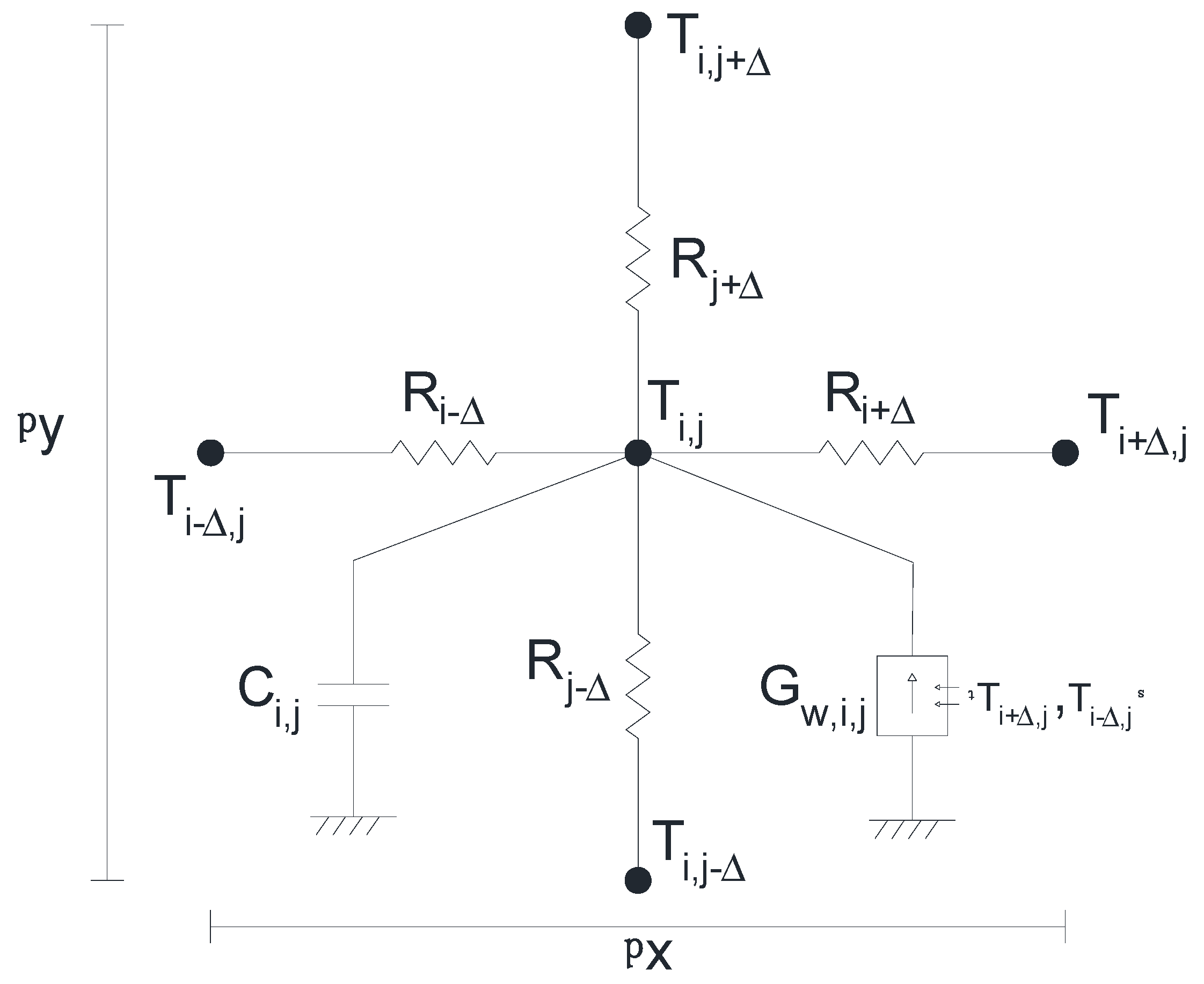
3.1. Elementary Cell for Vertical Flow

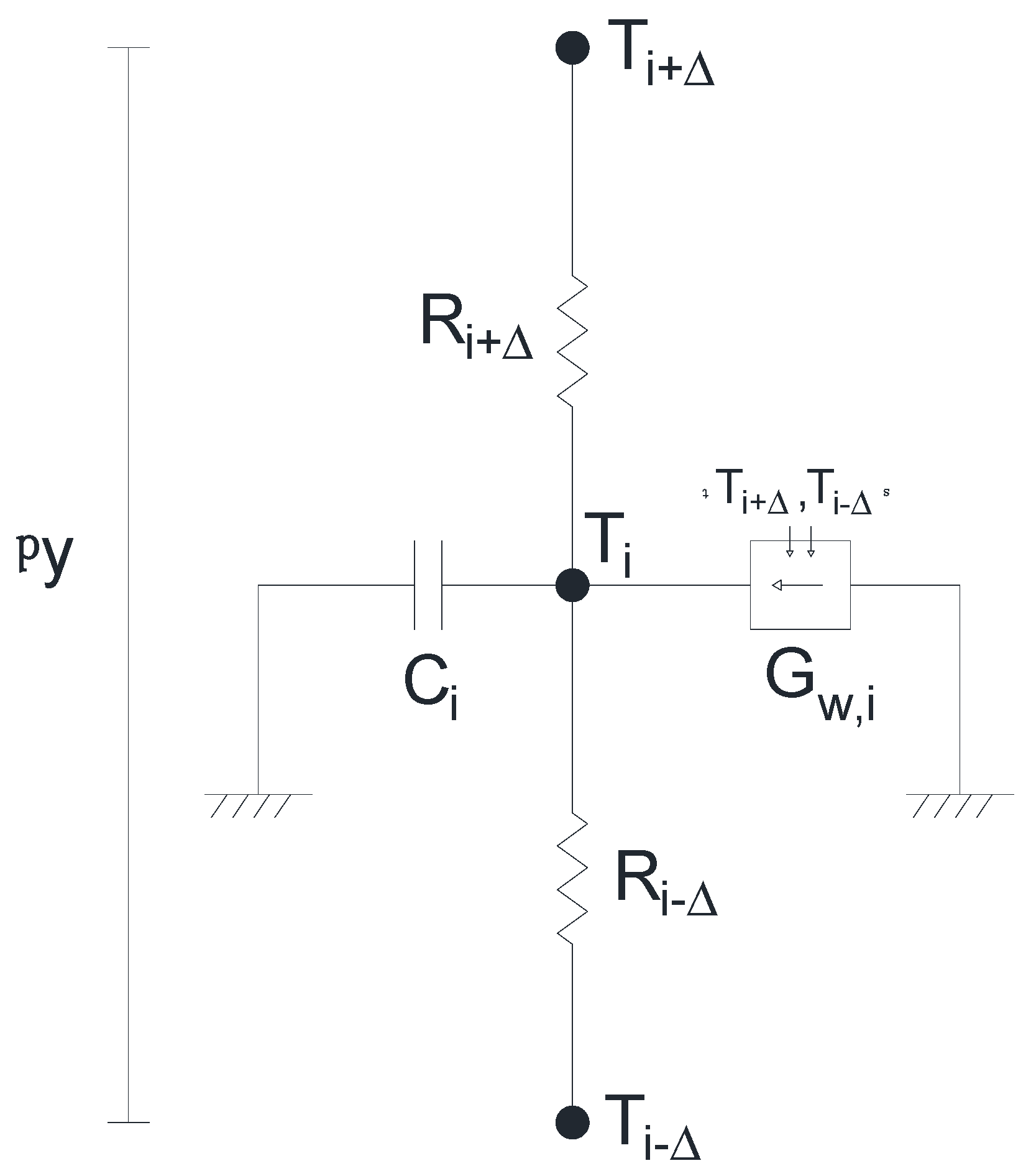
For the case of vertical flow, Equation (9) can be expressed in spatial finite differences (retaining time as a continuous variable) and, following the nomenclature of Figure 4, remains as follows:

$${\mathsf{\rho }}_{\mathrm{e}}{\mathrm{c}}_{\mathrm{e}}\frac{\partial \mathrm{T}}{\partial \mathrm{t}}={\mathrm{k}}_{\mathrm{m}}\left[\frac{{\mathrm{T}}_{\mathrm{i}+\Delta }-{\mathrm{T}}_{\mathrm{i}}}{\frac{\Delta {\mathrm{y}}^2}{2}}-\frac{{\mathrm{T}}_{\mathrm{i}}-{\mathrm{T}}_{\mathrm{i}-\Delta }}{\frac{\Delta {\mathrm{y}}^2}{2}}\right]-{\mathsf{\rho }}_{\mathrm{w}}{\mathrm{c}}_{\mathrm{w}}{\mathrm{q}}_{\mathrm{o},\mathrm{y}}\frac{{\mathrm{T}}_{\mathrm{i}+\Delta }-{\mathrm{T}}_{\mathrm{i}-\Delta }}{\Delta \mathrm{y}}$$

(13)

From the point of view of the network method, each addend of Equation (13) can be considered an electric current:

$${\mathrm{J}}_{\mathrm{c},\mathrm{e}}={\mathsf{\rho }}_{\mathrm{e}}{\mathrm{c}}_{\mathrm{e}}\frac{\partial \mathrm{T}}{\partial \mathrm{t}}, {\mathrm{J}}_{\mathrm{R}+\Delta }=\frac{{\mathrm{T}}_{\mathrm{i}+\Delta }-{\mathrm{T}}_{\mathrm{i}}}{\frac{{\left(\Delta \mathrm{y}\right)}^2}{2{\mathrm{k}}_{\mathrm{m}}}}, {\mathrm{J}}_{\mathrm{R}-\Delta }=\frac{{\mathrm{T}}_{\mathrm{i}}-{\mathrm{T}}_{\mathrm{i}-\Delta }}{\frac{{\left(\Delta \mathrm{y}\right)}^2}{2{\mathrm{k}}_{\mathrm{m}}}}, {\mathrm{J}}_{\mathrm{G},\mathrm{w}}={\mathsf{\rho }}_{\mathrm{w}}{\mathrm{c}}_{\mathrm{w}}{\mathrm{q}}_{\mathrm{o},\mathrm{y}}\frac{{\mathrm{T}}_{\mathrm{i}+\Delta }-{\mathrm{T}}_{\mathrm{i}-\Delta }}{\Delta \mathrm{y}}$$

(14)

which balance at the central node of the elementary cell, being:

$${\mathrm{J}}_{\mathrm{c},\mathrm{e}}={\mathrm{J}}_{\mathrm{R}+\Delta }-{\mathrm{J}}_{\mathrm{R}-\Delta }-{\mathrm{J}}_{\mathrm{G},\mathrm{w}}$$

(15)

In the network method, those linear terms such as ${\mathrm{J}}_{\mathrm{R}+\Delta }$ and ${\mathrm{J}}_{\mathrm{R}-\Delta }$ can be implemented by resistive-type devices. For this reason, and following Ohm’s law, $\mathrm{I}=\mathrm{V}/\mathrm{R}$, the values of the resistors can be expressed as:

$${\mathrm{R}}_{\mathrm{i}+\Delta }=\frac{{\left(\Delta \mathrm{y}\right)}^2}{2{\mathrm{k}}_{\mathrm{m}}}, {\mathrm{R}}_{\mathrm{i}-\Delta }=\frac{{\left(\Delta \mathrm{y}\right)}^2}{2{\mathrm{k}}_{\mathrm{m}}}$$

(16)

These elements, as shown in Figure 4, are located between the central node and one of the ends, which is where the potential fall occurs (in the physical analogy, the temperature). For its part, the linear term ${\mathrm{J}}_{\mathrm{c},\mathrm{e}}$, which includes a time derivative, can be implemented as a capacitor (${\mathrm{C}}_{\mathrm{i}}$) of ${\mathsf{\rho }}_{\mathrm{e}}{\mathrm{c}}_{\mathrm{e}}$ capacitance.

On the other hand, ${\mathrm{J}}_{\mathrm{G},\mathrm{w}}$ represents a non-linear term, which must be implemented in the circuit as voltage-controlled current source. In this element, the current is specified directly, by means of the following expressions:

$${\mathrm{G}}_{\mathrm{w},\mathrm{i}}={\mathsf{\rho }}_{\mathrm{w}}{\mathrm{c}}_{\mathrm{w}}{\mathrm{q}}_{\mathrm{o},\mathrm{y}}\frac{{\mathrm{T}}_{\mathrm{i}+\Delta }-{\mathrm{T}}_{\mathrm{i}-\Delta }}{\Delta \mathrm{y}}$$

(17)

where ${\mathrm{T}}_{\mathrm{i}+\Delta }$ and ${\mathrm{T}}_{\mathrm{i}-\Delta }$ are directly read at the extreme nodes of the corresponding cell i. This device, in the same way as the capacitor, must be implemented between the central node of the cell and the common ground node.

3.2. Elementary Cell for Regional Flow

For the case of regional flow, Equation (12) is expressed in spatial finite differences (retaining time as a continuous variable and following the nomenclature of Figure 5) as follows:

$${\mathsf{\rho }}_{\mathrm{e}}{\mathrm{c}}_{\mathrm{e}}\frac{\partial \mathrm{T}}{\partial \mathrm{t}}-{\mathrm{k}}_{\mathrm{m}}\left[\frac{{\mathrm{T}}_{\mathrm{i}+\Delta ,\mathrm{j}}-{\mathrm{T}}_{\mathrm{i},\mathrm{j}}}{\frac{\Delta {\mathrm{x}}^2}{2}}-\frac{{\mathrm{T}}_{\mathrm{i},\mathrm{j}}-{\mathrm{T}}_{\mathrm{i}-\Delta ,\mathrm{j}}}{\frac{\Delta {\mathrm{x}}^2}{2}}\right]-{\mathrm{k}}_{\mathrm{m}}\left[\frac{{\mathrm{T}}_{\mathrm{i},\mathrm{j}+\Delta }-{\mathrm{T}}_{\mathrm{i},\mathrm{j}}}{\frac{\Delta {\mathrm{y}}^2}{2}}-\frac{{\mathrm{T}}_{\mathrm{i},\mathrm{j}}-{\mathrm{T}}_{\mathrm{i},\mathrm{j}-\Delta }}{\frac{\Delta {\mathrm{y}}^2}{2}}\right]+{\mathsf{\rho }}_{\mathrm{w}}{\mathrm{c}}_{\mathrm{w}}{\mathrm{q}}_{\mathrm{o},\mathrm{x}}\frac{{\mathrm{T}}_{\mathrm{i}+\Delta ,\mathrm{j}}-{\mathrm{T}}_{\mathrm{i}-\Delta ,\mathrm{j}}}{\Delta \mathrm{x}}=0$$

(18)

Again, each addend of Equation (18) can be considered an electric current:

$${\mathrm{J}}_{\mathrm{R},\mathrm{i}+\Delta }=\frac{{\mathrm{T}}_{\mathrm{i}+\Delta ,\mathrm{j}}-{\mathrm{T}}_{\mathrm{i},\mathrm{j}}}{\frac{{\left(\Delta \mathrm{x}\right)}^2}{2{\mathrm{k}}_{\mathrm{m}}}}, {\mathrm{J}}_{\mathrm{R},\mathrm{i}-\Delta }=\frac{{\mathrm{T}}_{\mathrm{i},\mathrm{j}}-{\mathrm{T}}_{\mathrm{i}-\Delta ,\mathrm{j}}}{\frac{{\left(\Delta \mathrm{x}\right)}^2}{2{\mathrm{k}}_{\mathrm{m}}}},$$

$${\mathrm{J}}_{\mathrm{R},\mathrm{j}+\Delta }=\frac{{\mathrm{T}}_{\mathrm{i},\mathrm{j}+\Delta }-{\mathrm{T}}_{\mathrm{i},\mathrm{j}}}{\frac{{\left(\Delta \mathrm{y}\right)}^2}{2{\mathrm{k}}_{\mathrm{m}}}}, {\mathrm{J}}_{\mathrm{R},\mathrm{j}-\Delta }=\frac{{\mathrm{T}}_{\mathrm{i},\mathrm{j}}-{\mathrm{T}}_{\mathrm{i},\mathrm{j}-\Delta }}{\frac{{\left(\Delta \mathrm{y}\right)}^2}{2{\mathrm{k}}_{\mathrm{m}}}},$$

(19)

$${\mathrm{J}}_{\mathrm{c},\mathrm{e}}={\mathsf{\rho }}_{\mathrm{e}}{\mathrm{c}}_{\mathrm{e}}\frac{\partial \mathrm{T}}{\partial \mathrm{t}}, {\mathrm{J}}_{\mathrm{G},\mathrm{w},\mathrm{x}}={\mathsf{\rho }}_{\mathrm{w}}{\mathrm{c}}_{\mathrm{w}}{\mathrm{q}}_{\mathrm{o},\mathrm{x}}\frac{{\mathrm{T}}_{\mathrm{i}+\Delta ,\mathrm{j}}-{\mathrm{T}}_{\mathrm{i}-\Delta ,\mathrm{j}}}{\Delta \mathrm{x}}$$

which balance at the central node of the elementary cell, being:

$${\mathrm{J}}_{\mathrm{c},\mathrm{e}}-{\mathrm{J}}_{\mathrm{R},\mathrm{i}+\Delta }+{\mathrm{J}}_{\mathrm{R},\mathrm{i}-\Delta }-{\mathrm{J}}_{\mathrm{R},\mathrm{j}+\Delta }+{\mathrm{J}}_{\mathrm{R},\mathrm{j}-\Delta }+{\mathrm{J}}_{\mathrm{G},\mathrm{w},\mathrm{x}}=0$$

(20)

As seen before, the linear terms ${\mathrm{J}}_{\mathrm{R},\mathrm{i}+\Delta }$ and ${\mathrm{J}}_{\mathrm{R},\mathrm{i}-\Delta }$ can be implemented by resistors, whose values will be specified by:

$${\mathrm{R}}_{\mathrm{i}+\Delta }=\frac{{\left(\Delta \mathrm{x}\right)}^2}{2{\mathrm{k}}_{\mathrm{m}}}, {\mathrm{R}}_{\mathrm{i}-\Delta }=\frac{{\left(\Delta \mathrm{x}\right)}^2}{2{\mathrm{k}}_{\mathrm{m}}}$$

(21)

and will be placed between the central node and the right and left extreme nodes (Figure 5), respectively. For their part, the terms ${\mathrm{J}}_{\mathrm{R},\mathrm{j}+\Delta }$ and ${\mathrm{J}}_{\mathrm{R},\mathrm{j}-\Delta }$ are also modeled with both resistors, located between the central node and the upper and lower extreme nodes, respectively. Their values will come to be specified by:

$${\mathrm{R}}_{\mathrm{j}+\Delta }=\frac{{\left(\Delta \mathrm{y}\right)}^2}{2{\mathrm{k}}_{\mathrm{m}}}, {\mathrm{R}}_{\mathrm{j}-\Delta }=\frac{{\left(\Delta \mathrm{y}\right)}^2}{2{\mathrm{k}}_{\mathrm{m}}}$$

(22)

As for the case of vertical flow, the linear storage term ${\mathrm{J}}_{\mathrm{c},\mathrm{e}}$ is implemented by means of a capacitor (${\mathrm{C}}_{\mathrm{i},\mathrm{j}}$), whose capacitance value is ${\mathsf{\rho }}_{\mathrm{e}}{\mathrm{c}}_{\mathrm{e}}$.

Finally, the non-linear term ${\mathrm{J}}_{\mathrm{G},\mathrm{w}}$ will be implemented by the voltage-controlled current source ${\mathrm{G}}_{\mathrm{w},\mathrm{i},\mathrm{j}}$, defined by:

$${\mathrm{G}}_{\mathrm{w},\mathrm{i},\mathrm{j}}={\mathsf{\rho }}_{\mathrm{w}}{\mathrm{c}}_{\mathrm{w}}{\mathrm{q}}_{\mathrm{o},\mathrm{x}}\frac{{\mathrm{T}}_{\mathrm{i}+\Delta ,\mathrm{j}}-{\mathrm{T}}_{\mathrm{i}-\Delta ,\mathrm{j}}}{\Delta \mathrm{x}}$$

(23)

where ${\mathrm{T}}_{\mathrm{i}+\Delta ,\mathrm{j}}$ and ${\mathrm{T}}_{\mathrm{i}-\Delta ,\mathrm{j}}$ are directly read at the right and left extreme nodes of the corresponding cell i,j. This device is implemented between the central node of the cell and the common ground node, in the same way as the capacitor.

3.3. Boundary and Initial Conditions

Both for the cases of regional flow and exclusively vertical flow, the only initial condition to implement is that of the initial ground temperature (${\mathrm{T}}_{\mathrm{s}}$), Equation (8). In the network method, this condition is very easy to establish, since it is only necessary to indicate what is the initial voltage at which the capacitors (${\mathrm{C}}_{\mathrm{i}}$ or ${\mathrm{C}}_{\mathrm{i},\mathrm{j}}$) are charged.

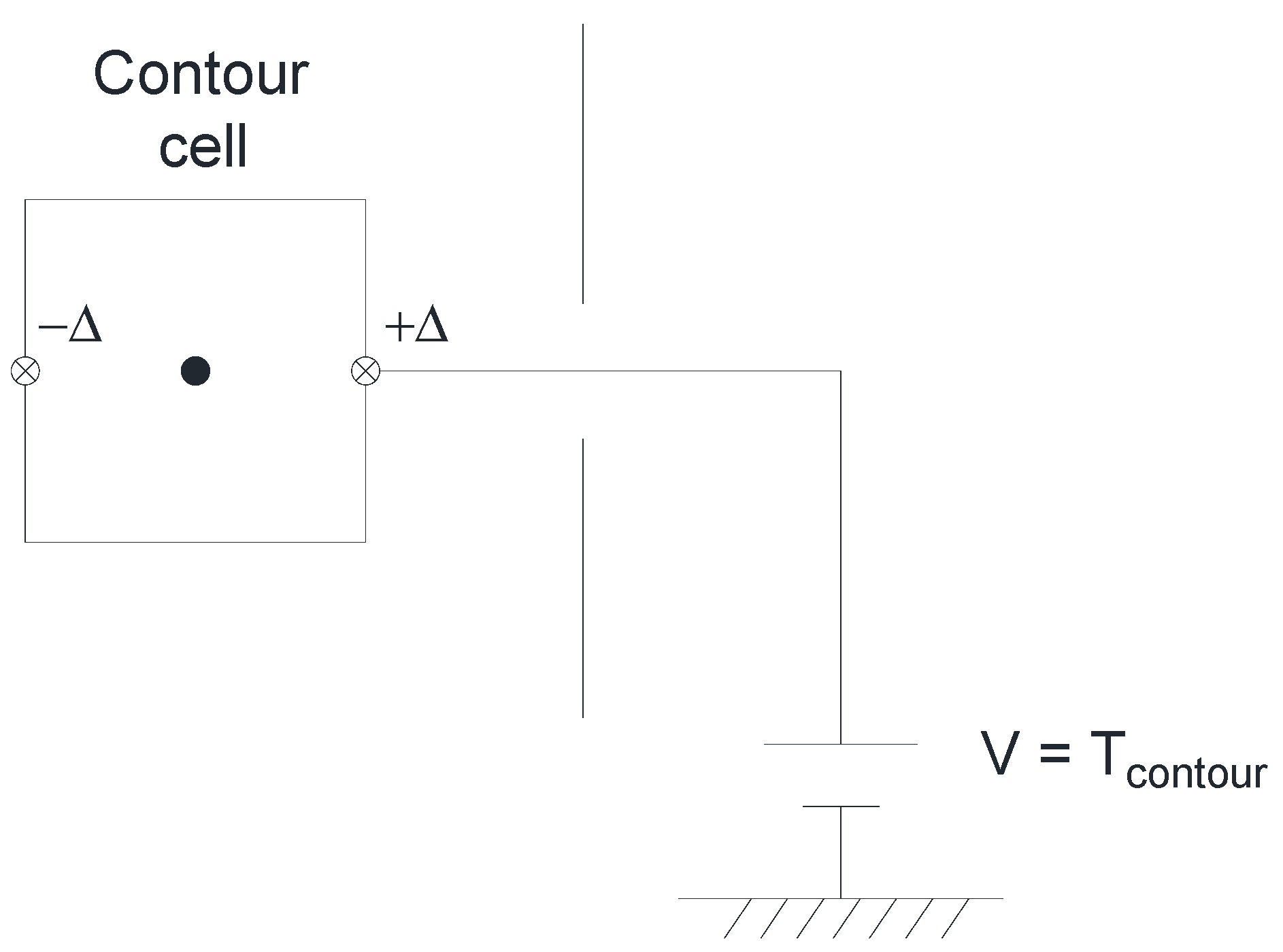
Regarding the boundary conditions, in those cases where the temperature of the contour remains invariant, Equations (3)–(5), it is enough to place a voltage source (${\mathrm{V}}_{\mathrm{i}}$ or ${\mathrm{V}}_{\mathrm{i},\mathrm{j}}$) of constant value, connected from the corresponding contour node to the common ground node, as can be seen in Figure 6.

For those cases in which it is desired that the temperature of the soil surface varies in a stepwise manner, the network method allows the implementation of a stepped function in a simple way, by means of a function commonly called PULSE [42,43]. In this case, the value of the voltage source (${\mathrm{V}}_{\mathrm{i}}$ or ${\mathrm{V}}_{\mathrm{i},\mathrm{j}}$) will vary with time, as shown in Figure 2, between ${\mathrm{T}}_1$ and ${\mathrm{T}}_2$, depending on the values assigned to the parameters (Table 2) necessary to define the PULSE function: ${\mathrm{T}}_{\mathrm{D}}$, ${\mathrm{T}}_{\mathrm{R}}$, ${\mathrm{P}}_{\mathrm{W}}$, ${\mathrm{T}}_{\mathrm{F}}$ and $\mathrm{P}$.

Finally, for the case of sinusoidal variation of the ground surface temperature (Figure 3), the specific sinusoidal function [31,32] has been used, which defines the instantaneous value of the potential (that is, the temperature) provided by the voltage source. In this case, the parameters to be specified are: ${\mathrm{T}}_{\mathrm{m}}$ and ${\mathrm{T}}_{\sin }$ (Table 3 and Table 4).

4. Verification of the Model and Applications

In this section, a total of four applications will be presented that will serve both to validate the precision of our models and to illustrate a series of scenarios that can be found in real practical situations of heat transport in saturated porous media in which exists, at the same time, a flow of water.

4.1. Verification of the Model. Constant Surface Temperature and Different Vertical Flow Rates

This first application aims to show the high precision that is achieved with the network method in obtaining the numerical solution to this type of problem. The model addressed is that of exclusively vertical flow with constant temperature on the ground surface, as described in Section 2.1.1. For this scenario,

Table 5. Parameters of the scenario with constant surface temperature. Vertical flow.

Parameter	Value	Units
${\mathrm{k}}_{\mathrm{m}}$	0.84	J/(sm °C)
${\mathsf{\rho }}_{\mathrm{e}}{\mathrm{c}}_{\mathrm{e}}$	4.20 × 106	J/(m3 °C)
${\mathsf{\rho }}_{\mathrm{w}}{\mathrm{c}}_{\mathrm{w}}$	4.20 × 106	J/(m3 °C)
$\mathrm{H}$	1	m
$\mathrm{n}$	100
Cell height ($\Delta \mathrm{y}$)	0.01	m

summarizes the geometric parameters of the problem, as well as the thermal properties of the porous medium, while Table 1 does it with the conditions of initial temperature of the soil and in the lower and upper contours.

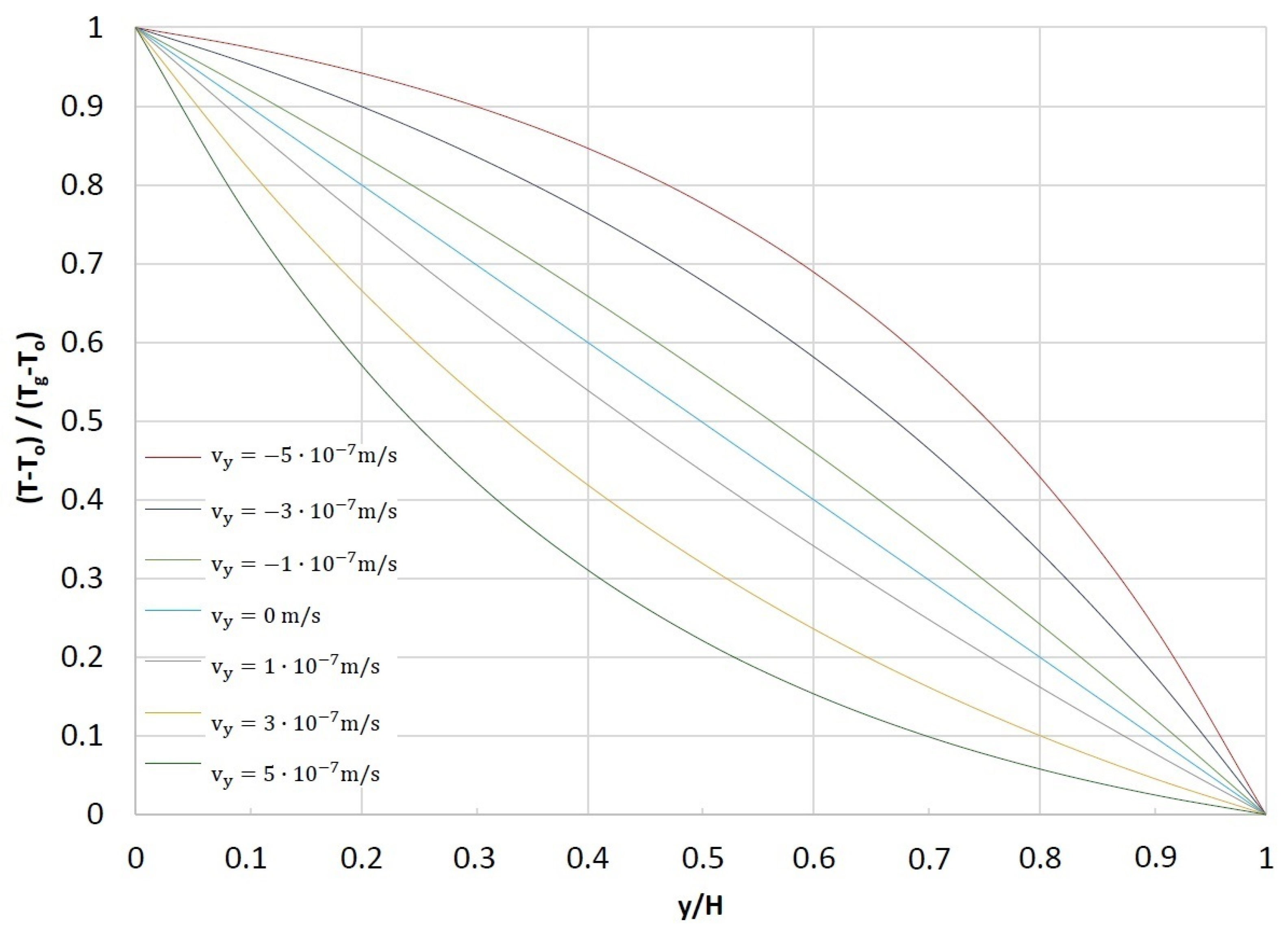
In Figure 7, the values of the temperature $\mathrm{T}$ are represented as a function of the depth $\mathrm{Y}$, once the steady state has been reached and for different values and directions of the vertical velocity ${\mathrm{v}}_{\mathrm{y}}$: upward flow (positive ${\mathrm{v}}_{\mathrm{y}}$), downward flow (negative ${\mathrm{v}}_{\mathrm{y}}$) and non-existent flow (${\mathrm{v}}_{\mathrm{y}}$ equal to 0). As can be seen, and due to the fact that the temperature of the bottom edge is lower than that of the ground surface, for the cases of upward flow there is a cooling of the medium (taking the case of null flow as a reference), the more pronounced, the higher the velocity ${\mathrm{v}}_{\mathrm{y}}$, while for the cases of downward flow, what is observed is a warming of the medium.

The results presented here coincide with the analytical solutions presented by Bredehoeft and Papaopulos [7] and satisfactorily approximate the data collected in the in situ study carried out by Duque et al. [2] in the coastal lagoon of Ringkøbing Fjord (Denmark), as shown in

Table 6. Comparative results between the network method solution, the in situ and fitted real data of Duque et al. (2016) [2] and the analytical solution of Bredehoeft and Papaopulos [7]. Constant surface temperature case and upward flow (${\mathrm{v}}_{\mathrm{y}}=5·{10}^{-7}$ m/s.

	y (m)	0	0.025	0.05	0.075	0.10	0.15	0.20	0.25	0.35	0.50
Network method (NM)	T (°C)	22.35	21.4	20.51	19.67	18.89	17.46	16.19	15.08	13.23	11.19
Duque et al. (2016) in situ	T (°C)	22.35	22.3	21.35	20.20	19.25	17.90	16.45	14.05	12.6	12.1
	NM relative error (%)	0.00	4.04	3.93	2.61	1.89	2.49	1.57	7.31	4.97	7.53
Fitted Duque et al. (2016)	T (°C)	22.00	21.30	20.60	19.80	19.00	17.50	16.00	14.50	12.85	11.75
	NM relative error (%)	1.59	0.47	0.44	0.65	0.59	0.26	1.20	3.98	2.93	4.77
Bredehoeft and Papaopulos (1965) analytical solution	T (°C)	22.35	21.50	20.55	19.75	18.89	17.45	16.21	15.10	13.25	11.24
	NM relative error (%)	0.00	0.47	0.19	0.39	0.01	0.03	0.09	0.15	0.18	0.44

. As can be seen, the maximum relative error is 7.53% when compared with the real data of Duque et al. [2], although this is considerably reduced to 4.77% when compared with their fitted curve. On the other hand, when we compare with the analytical solution proposed by Bredehoeft and Papaopulos [7], the maximum relative error does not exceed 0.47%. Without a doubt, these are very low errors for the engineering field, which shows that the solutions obtained with our tool are highly accurate and valid for the simulation of real scenarios.

It should be noted that the number of cells into which the medium has been divided is 100 (Table 5), a mesh for which values of the temperature variable have been obtained with maximum relative errors below 0.5%, in comparison with the temperatures provided by Bredehoeft and Papaopulos [7], Table 6. A mesh sensitivity analysis is presented in

Table 7. Network method maximum relative errors and calculation times according to the number of cells.

Cells Number (n)	Max. Relative Error (%)	Calculation Time (s)
10	23.91	3
20	6.21	7
50	0.96	15
100	0.47	29
200	0.34	114

, which shows the maximum relative error made by our approximation (taking as reference the analytical solutions [7]) as a function of the number of cells, as well as calculation times. As can be seen, the network method achieves very precise solutions with undemanding grids, since with meshes above 50 cells, the maximum relative error does not exceed 1%. On the other hand, above 100 cells, more demanding meshes hardly reduce the error, while computing times are significantly affected. Therefore, we consider a 100 cell mesh to be suitable.

4.2. Stepped Surface Temperature and Different Vertical Flow Rates

In this case, the model addressed is the one described in Section 2.1.2, with exclusively vertical flow and stepped temperature variation on the soil surface.

Table 8. Parameters of the scenario with stepped surface temperature. Vertical flow.

Parameter	Value	Units
${\mathrm{k}}_{\mathrm{m}}$	0.84	J/(sm °C)
${\mathsf{\rho }}_{\mathrm{e}}{\mathrm{c}}_{\mathrm{e}}$	3.55 × 106	J/(m3 °C)
${\mathsf{\rho }}_{\mathrm{w}}{\mathrm{c}}_{\mathrm{w}}$	4.18 × 106	J/(m3 °C)
$\mathrm{H}$	2	m
$\mathrm{n}$	100
Cell height ($\Delta \mathrm{y}$)	0.02	m

shows the geometric parameters of the problem and the thermal properties of the ground for this case. On the other hand, Table 2 summarizes the temperature conditions in the lower and upper contours (with the different parameters necessary to define the stepped temperature function), as well as the initial temperature of the medium.

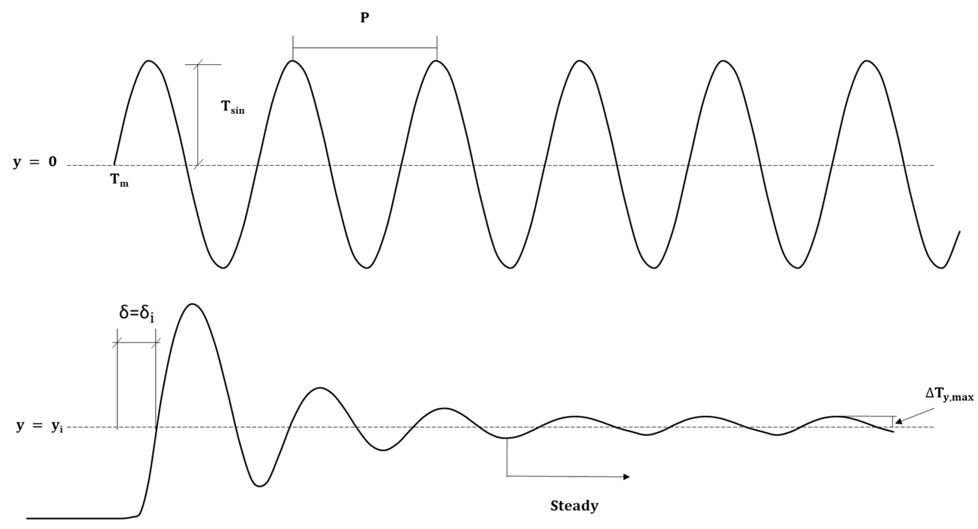
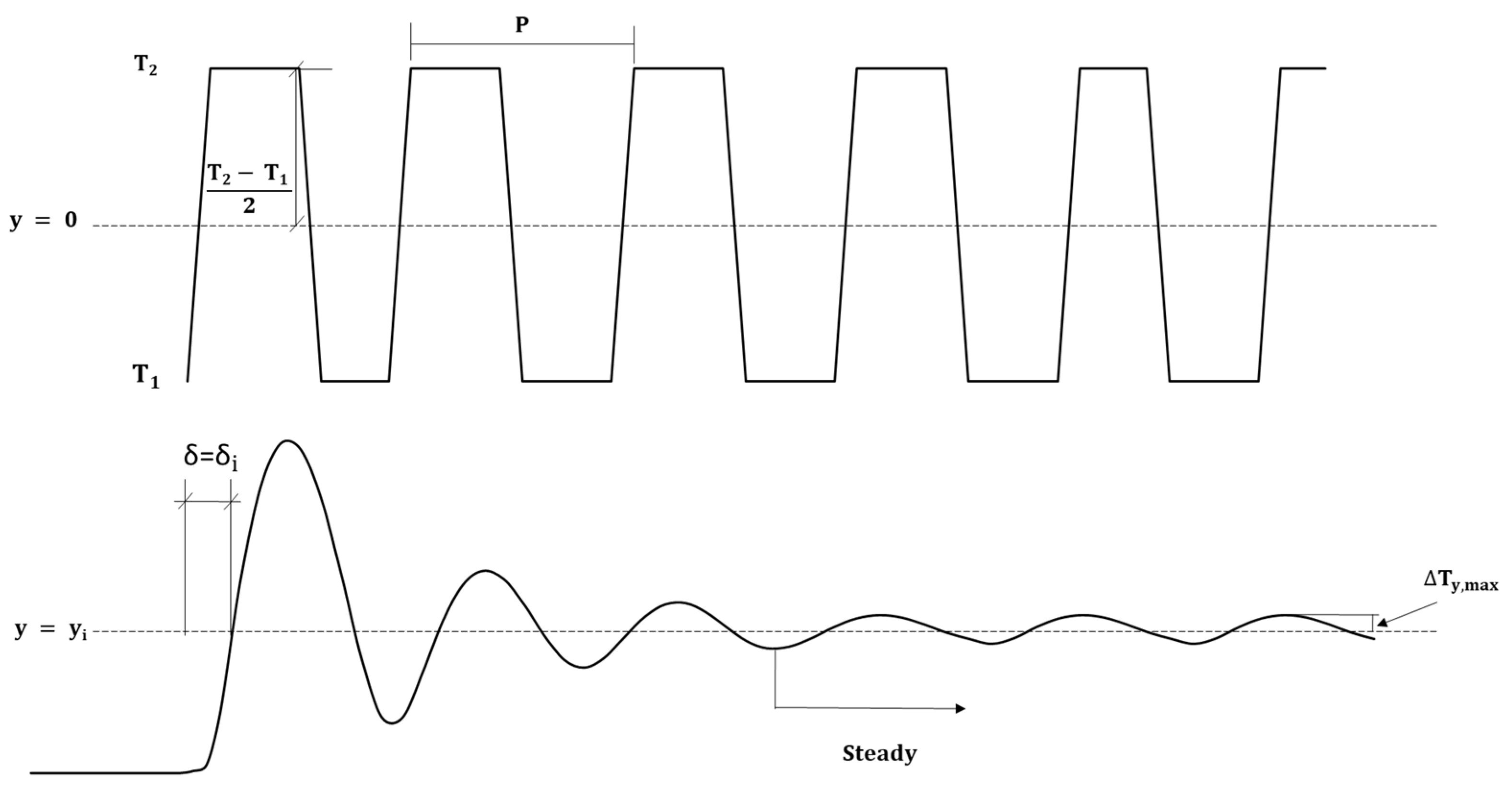
Figure 8 schematizes how the steady state is reached, at a certain depth ${\mathrm{y}}_{\mathrm{i}}$, after the start of the problem, for the case of stepped surface temperature. Once this state is reached, it is observed that the temperature is not constant, but fluctuates between certain values in wave form, the variable $\Delta {\mathrm{T}}_{\mathrm{y},\max }$ being the amplitude of that wave.

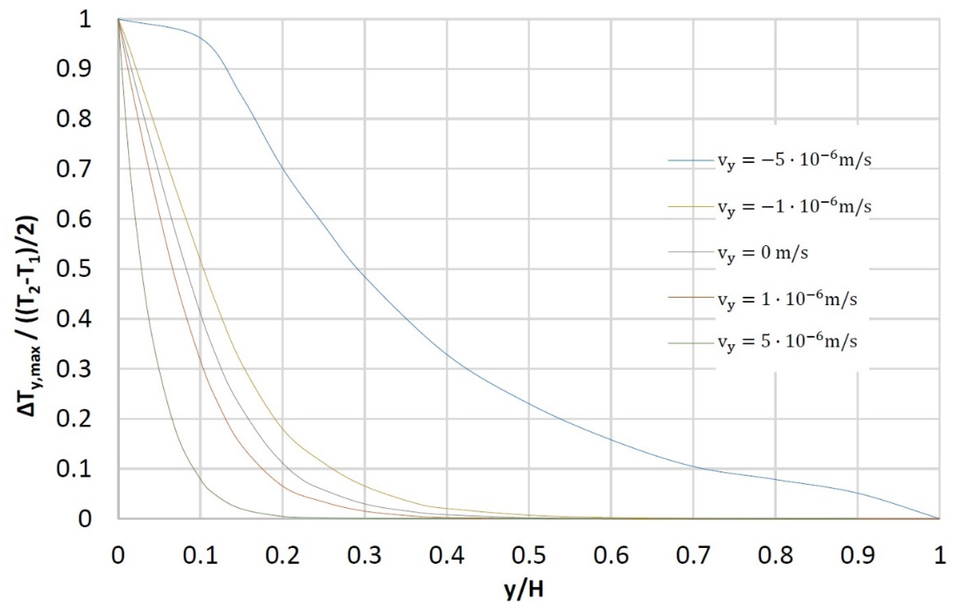
Figure 9 represents the amplitude ($\Delta {\mathrm{T}}_{\mathrm{y},\max }$) that the temperature steady wave reaches, as a function of the depth $\mathrm{Y}$, for different values and directions of the vertical velocity ${\mathrm{v}}_{\mathrm{y}}$: upward flow (positive ${\mathrm{v}}_{\mathrm{y}}$), downward flow (negative ${\mathrm{v}}_{\mathrm{y}}$) and non-existent flow (${\mathrm{v}}_{\mathrm{y}}$ equal to 0). As can be seen (for the specific values of the initial and boundary conditions of temperature, Table 2), as in the previous application, a cooling of the medium occurs when the water flow is upward (taking the ${\mathrm{v}}_{\mathrm{y}}=0$ case as a reference), of greater magnitude the greater the velocity ${\mathrm{v}}_{\mathrm{y}}$, while a warming of the medium is manifested when the flow is downward. The mesh used for this application was also 100 cells, which has proven sufficient to achieve high precision with the network method in this type of problem.

4.3. Sinusoidal Surface Temperature and Different Vertical Flow Rates

Now, the scenario addressed corresponds to a case of exclusively vertical flow with sinusoidal temperature variation on the ground surface (as described in Section 2.1.3), whose geometric parameters and thermal properties of the porous medium are summarized in

Table 9. Parameters of the scenario with sinusoidal surface temperature. Vertical flow.

Parameter	Value	Units
${\mathrm{k}}_{\mathrm{m}}$	0.84	J/(sm °C)
${\mathsf{\rho }}_{\mathrm{e}}{\mathrm{c}}_{\mathrm{e}}$	3.55 × 106	J/(m3 °C)
${\mathsf{\rho }}_{\mathrm{w}}{\mathrm{c}}_{\mathrm{w}}$	4.18 × 106	J/(m3 °C)
$\mathrm{H}$	1	m
$\mathrm{n}$	100
Cell height ($\Delta \mathrm{y}$)	0.01	m

. The initial and boundary temperature conditions are summarized in Table 3.

Figure 10 shows schematically how the steady state is reached (at a certain depth ${\mathrm{y}}_{\mathrm{i}}$) after the start of the problem, for the case of sinusoidal surface temperature. In the stationary situation, it is observed how the temperature is not constant, but oscillates in the form of a wave between certain values, the variable $\Delta {\mathrm{T}}_{\mathrm{y},\max }$ being the amplitude of such a wave.

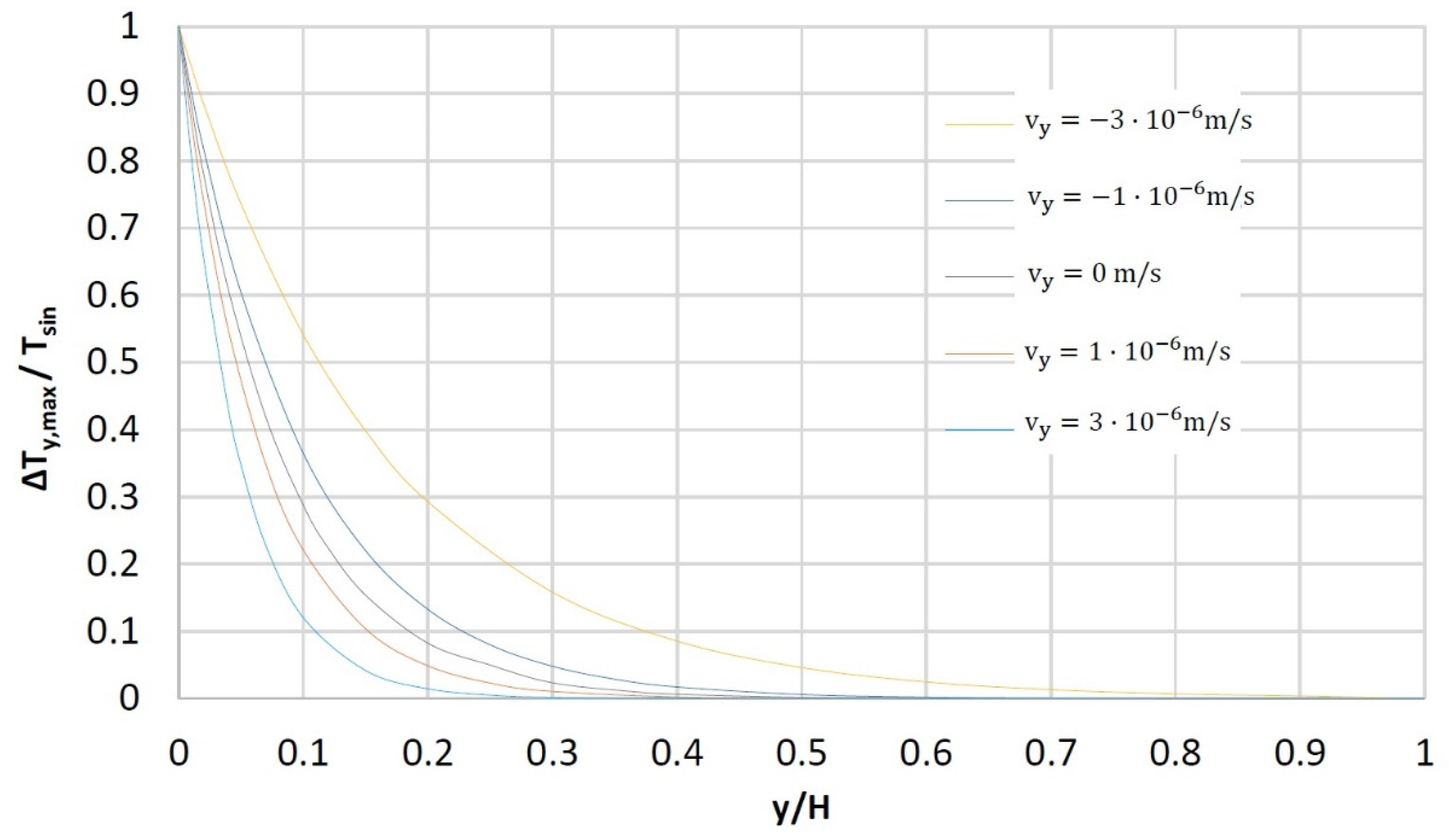
Figure 11 represents the amplitude ($\Delta {\mathrm{T}}_{\mathrm{y},\max }$) that the temperature steady wave reaches, as a function of the depth $\mathrm{Y}$, for different values and directions of the vertical velocity ${\mathrm{v}}_{\mathrm{y}}$. As in the previous applications (and for the specific values, reflected in Table 3, of the initial and boundary temperature conditions), upflows induce a cooling of the medium (taking the ${\mathrm{v}}_{\mathrm{y}}=0$ case as a reference), of greater magnitude as we increase ${\mathrm{v}}_{\mathrm{y}}$. For downflows, the effect is the opposite (increased temperatures). The simulations were performed again with a 100 cell grid.

4.4. Sinusoidal Surface Temperature and Regional Flow

Finally, we address a scenario where the temperature at the ground surface varies sinusoidally but where the flow is, on this occasion, horizontal (as described in Section 2.2). The boundary conditions and the initial soil temperature are summarized in Table 4, while the medium thermal properties and the geometry of the domain (2D) are collected in

Table 10. Parameters of the scenario with sinusoidal surface temperature. Regional flow.

Parameter	Value	Units
${\mathrm{k}}_{\mathrm{m}}$	0.84	J/(sm °C)
${\mathsf{\rho }}_{\mathrm{e}}{\mathrm{c}}_{\mathrm{e}}$	3.55 × 10−6	J/(m3 °C)
${\mathsf{\rho }}_{\mathrm{w}}{\mathrm{c}}_{\mathrm{w}}$	4.18 × 10−6	J/(m3 °C)
$\mathrm{H}$	1	m
Cell height ($\Delta \mathrm{y}$)	0.05	m
$\mathrm{L}$	30	m
Cell width ($\Delta \mathrm{x}$)	0.3	m
${\mathrm{v}}_{\mathrm{x}}={\mathrm{q}}_{\mathrm{o},\mathrm{x}}$	3 × 10−5	m/s
${\mathrm{n}}_{\mathrm{y}}$	20
${\mathrm{n}}_{\mathrm{x}}$	100

. In this sense, it should be noted that a scenario with horizontal water flow from left to right has been chosen, so that the heat existing in the left lateral contour of the problem is transported by the water flow to the porous medium. Regarding its dimensions, a length large enough has been chosen so that there are areas of the porous medium that are not affected by this boundary condition. In this way, we can analyze the effect that the variation in surface temperature has on the porous medium both in the vicinity of the lateral heat source and in distant locations. The chosen grid has been 100 cells in the flow direction (horizontal) by 20 cells vertically (as there is no flow component in that direction, the mesh can be much less demanding).

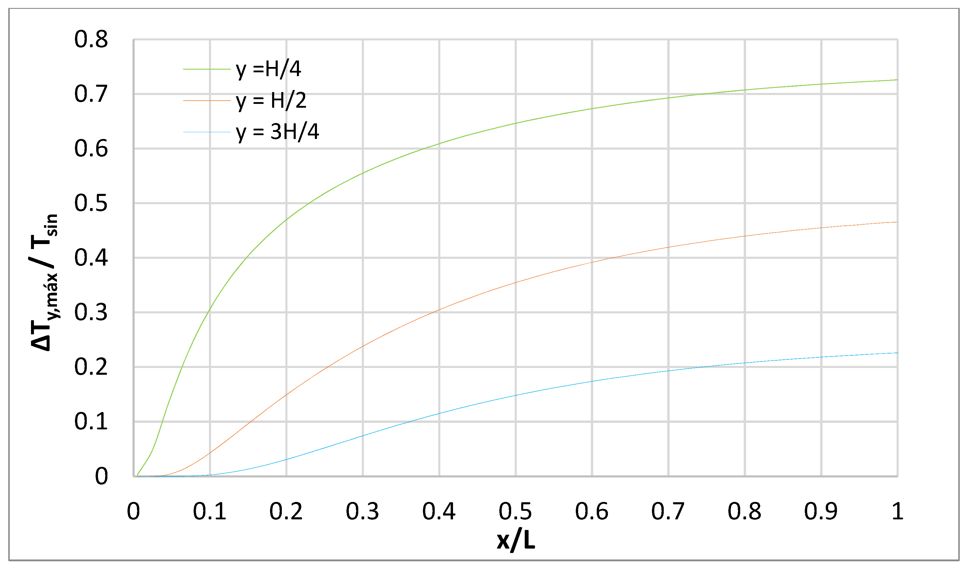
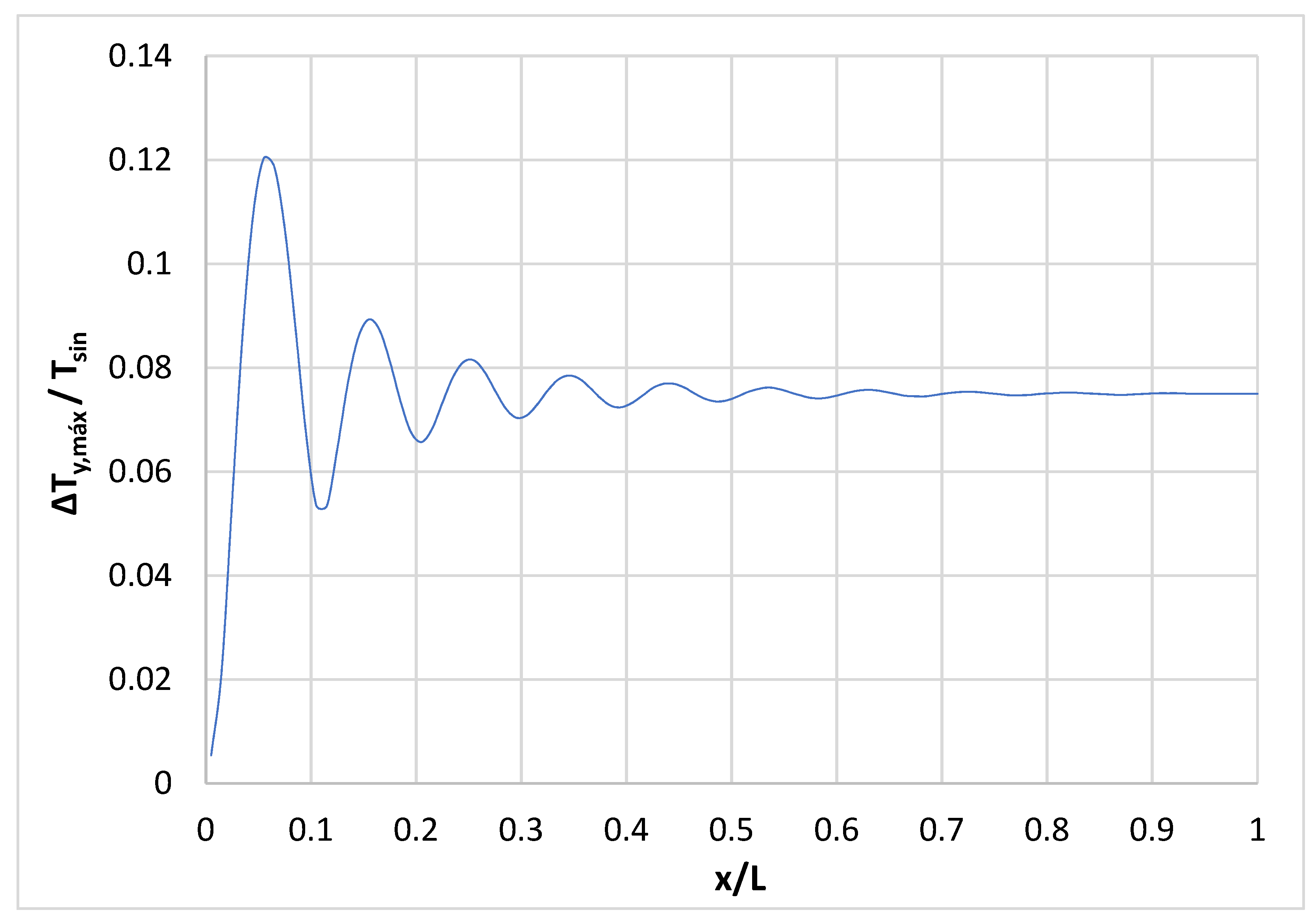
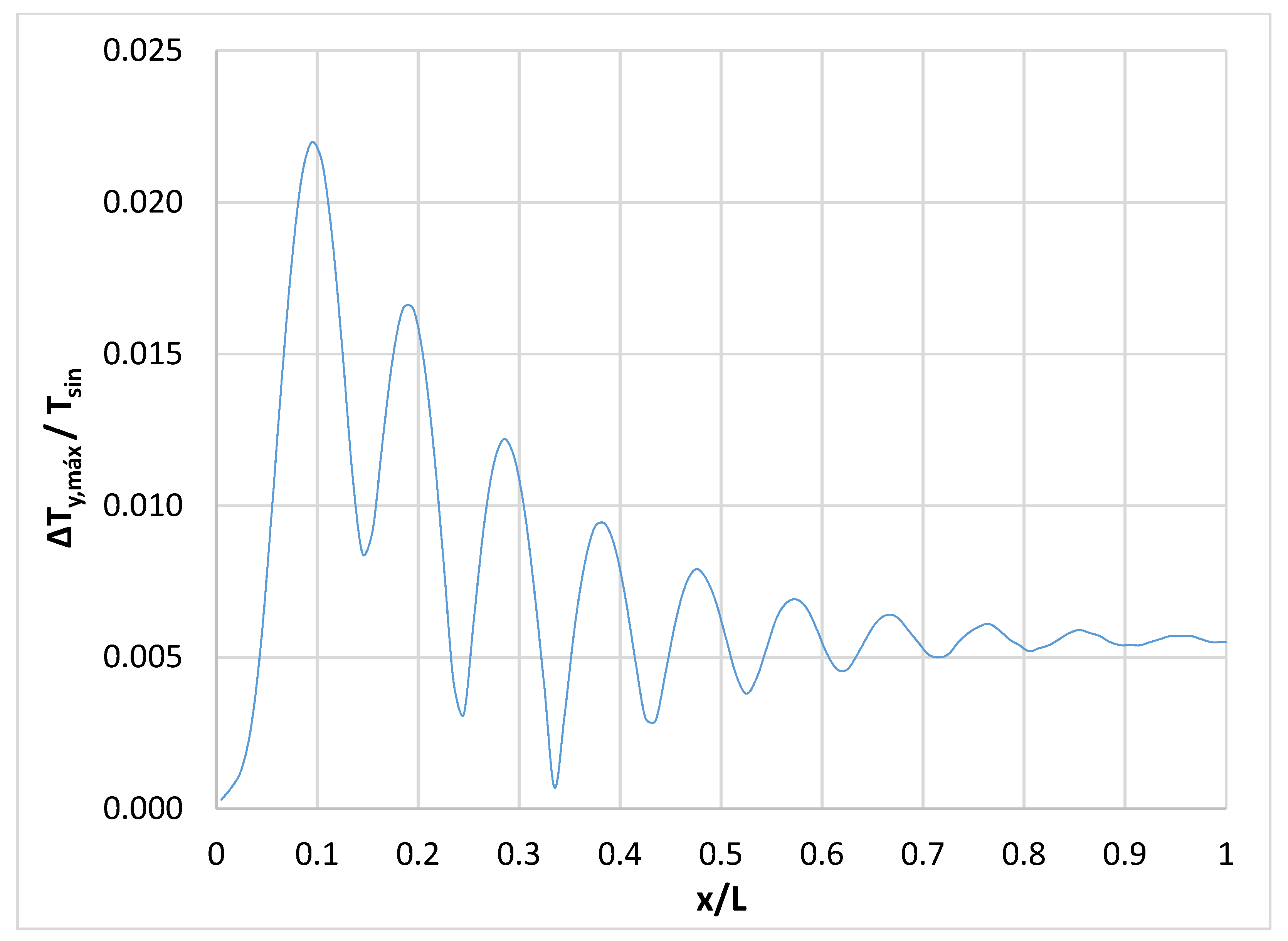
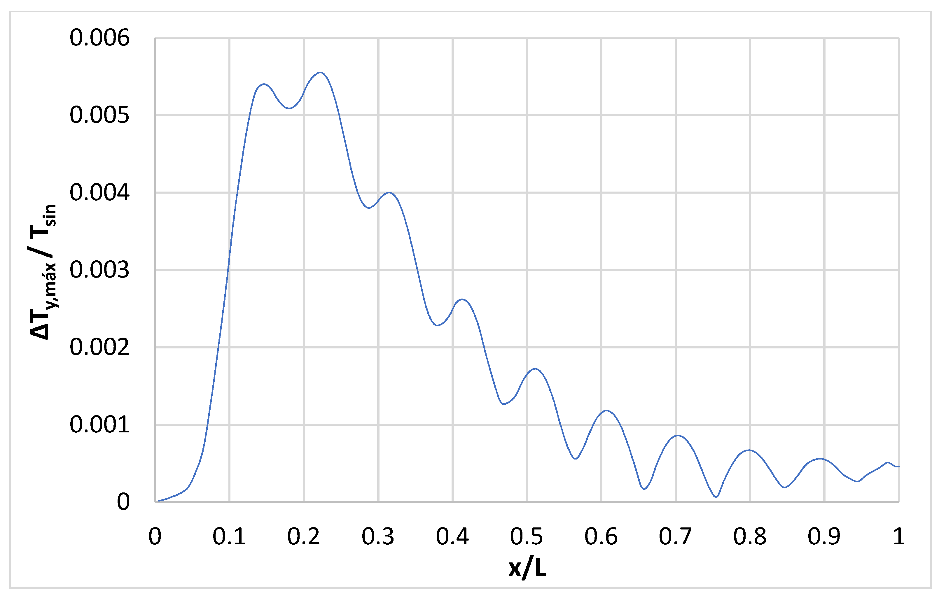
Figure 12, Figure 13 and Figure 14 represent the amplitude ($\Delta {\mathrm{T}}_{\mathrm{y},\max }$) that the temperature steady wave reaches, as a function of the length X of the domain, for different values of the depth ($\mathrm{H}/4$, $\mathrm{H}/2$ and $3\mathrm{H}/4$). For this case, with a daily period ($\mathrm{P}$) of the sinusoidal wave of surface temperature, it is observed as the amplitude ($\Delta {\mathrm{T}}_{\mathrm{y},\max }$) that reaches the steady wave of temperature in the ground; it is not very significant (less than 8% of the amplitude of the surface temperature sinusoidal wave at a distance of $\mathrm{H}/4$ from the surface), being even lower at those depths far from the surface.

This is due to the fact that the heat drag component has a great importance compared to the diffusive one (the regional flow velocity, ${\mathrm{v}}_{\mathrm{x}}$, is quite high while the heat conductivity of the rock-fluid matrix, ${\mathrm{k}}_{\mathrm{m}}$, presents a relatively low value), so that, for the values of lateral temperature (entry to the domain) and sinusoidal surface function, Table 4, the variation of the porous medium temperature due to the effect of the surface temperature is minimized by the drag effects.

However, when the period ($\mathrm{P}$) of the surface temperature sinusoidal wave is annual, the amplitude ($\Delta {\mathrm{T}}_{\mathrm{y},\max }$) reached by the steady temperature wave in the medium does become significant (about 75% of the amplitude of the surface temperature sinusoidal wave, at a distance of $\mathrm{H}/4$ from the surface), descending, logically, as we move away from the surface, Figure 15. On this occasion, the increase in the period of the surface temperature wave contributes to the diffusive process, so that the drag and diffusion components are more balanced in this case.

5. Conclusions

The network method has been revealed as an optimal tool for the numerical modeling and simulation of heat transport problems with water flow coupling in porous media. Its high versatility has made it possible to approach, in a simple way, both one-dimensional models with exclusively vertical heat transport and water flow and more complex regional flow models where it is necessary to resort to two-dimensional geometries.

From the analogy established between the temperature of the porous medium and the electrical potential of the equivalent circuit, the main physical phenomena that occur in the problem, in the form of terms or addends of the differential governing equation, are perfectly reproduced in the network model through the different electrical components that make up the equivalent circuit. Thus, the capacitors have served to implement both the initial temperature of the porous medium and the heat storage process of the ground throughout the simulation. For their part, electrical resistors govern the heat diffusion phenomenon, based on the heat conductivity of the rock-fluid matrix and the size of the elementary cell. The heat drag effects caused by the coupled water flow have been modeled using current sources, which collect properties such as density and specific heat, as well as the velocity of the water flow. Finally, the temperature boundary conditions (constant, stepped or sinusoidal) are easily implemented by voltage sources, duly placed in the corresponding contour nodes.

The network model proposed here has been successfully verified through a 1D application in which the water flow is exclusively vertical. The temperature-depth profiles obtained have been compared with the analytical solutions available in the scientific literature, verifying that the solutions provided by our tool coincide with these, leaving the relative errors dependent on the size of the chosen mesh: relative errors below 1% for meshes above 50 cells, decreasing below 0.5% when the number of cells increases to 100. For all this, the network method is revealed as a powerful numerical tool, in addition to being fast and simple, in the simulation of this type of problem.

Finally, and once the precision of our model has been demonstrated, a series of scenarios, both in 1D (vertical flow) and 2D (horizontal flow) domains and with different temperature conditions of the ground surface, has been addressed in order to illustrate the versatility of our tool, obtaining the ranges of values (in the form of maximum amplitudes) between which the temperature fluctuates at a certain depth and/or position of the porous medium.

In future research, the model presented here could be extended to problems where the properties of the porous medium change over time (swelling and erosion processes), soils with non-homogenous thermal and hydraulic characteristics or other surface temperature functions, different from those presented here, including tabulated data from actual temperature distributions.

References

- Constantz, D.A.; Stonestrom, J. Heat as a tracer of water movement near streams. US Geol. Surv. Circ. 2003, 1260, 1–96. [Google Scholar]
- Duque, C.; Müller, S.; Sebok, E.; Haider, K.; Engesgaard, P. Estimating groundwater discharge to surface waters using heat as a tracer in low flux environments: The role of thermal conductivity. Hydrol. Process. 2016, 30, 383–395. [Google Scholar] [CrossRef]
- Su, J.; Jasperse, G.W.; Seymour, J.; Constantz, D. Estimation of Hydraulic Conductivity in an Alluvial System Using Temperatures—ProQuest. Ground Water 2004, 42, 890–901. Available online: https://www.proquest.com/openview/88f86e0bc8f8376756ac2888c63e7408/1?pq-origsite=gscholar&cbl=48478 (accessed on 6 July 2021).
- Domenico, V.V.; Palciauskas, P.A. Theoretical Analysis of Forced Convective Heat Transfer in Regional Ground-Water Flow | GSA Bulletin | GeoScienceWorld. Geol. Soc. Am. Bull. 1973, 84, 3803–3814. [Google Scholar] [CrossRef]
- Reiter, M.; Costain, J.K.; Minier, J. Heat flow data and vertical groundwater movement, examples from southwestern Virginia. J. Geophys. Res. 1989, 94, 12423–12431. [Google Scholar] [CrossRef]
- Mansure, A.J.; Reiter, M. A vertical groundwater movement correction for heat flow. J. Geophys. Res. 1979, 84, 3490–3496. [Google Scholar] [CrossRef]
- Bredehoeft, J.D.; Papaopulos, I.S. Rates of vertical groundwater movement estimated from the Earth’s thermal profile. Water Resour. Res. 1965, 1, 325–328. [Google Scholar] [CrossRef]
- Stallman, R.W. Steady one-dimensional fluid flow in a semi-infinite porous medium with sinusoidal surface temperature. J. Geophys. Res. 1965, 70, 2821–2827. [Google Scholar] [CrossRef]
- Suzuki, S. Percolation measurements based on heat flow through soil with special reference to paddy fields. J. Geophys. Res. 1960, 65, 2883–2885. [Google Scholar] [CrossRef]
- Taniguchi, M. Evaluation of vertical groundwater fluxes and thermal properties of aquifers based on transient temperature-depth profiles. Water Resour. Res. 1993, 29, 2021–2026. [Google Scholar] [CrossRef]
- Taniguchi, M.; Sharma, M.L. Determination of groundwater recharge using the change in soil temperature. J. Hydrol. 1993, 148, 219–229. [Google Scholar] [CrossRef]
- Horton, C.W.; Rogers, F.T. Convection currents in a porous medium. J. Appl. Phys. 1945, 16, 367–370. [Google Scholar] [CrossRef]
- Lapwood, E.R. Convection of a fluid in a porous medium. Math. Proc. Camb. Philos. Soc. 1948, 44, 508–521. [Google Scholar] [CrossRef]
- Wooding, R.A. Steady state free thermal convection of liquid in a saturated permeable medium. J. Fluid Mech. 1957, 2, 273–285. [Google Scholar] [CrossRef]
- Cheng, P. Heat Transfer in Geothermal Systems. Adv. Heat Transf. 1979, 14, 1–105. [Google Scholar] [CrossRef]
- Ciriello, V.; Bottarelli, M.; di Federico, V.; Tartakovsky, D.M. Temperature fields induced by geothermal devices. Energy 2015, 93, 1896–1903. [Google Scholar] [CrossRef] [Green Version]
- Tirado-Conde, J.; Engesgaard, P.; Karan, S.; Müller, S.; Duque, C. Evaluation of temperature profiling and seepage meter methods for quantifying submarine groundwater discharge to coastal lagoons: Impacts of saltwater intrusion and the associated thermal regime. Water 2019, 11, 1648. [Google Scholar] [CrossRef] [Green Version]
- Mastrocicco, M.; Soana, E.; Colombani, N.; Vincenzi, F.; Castaldi, S.; Castaldelli, G. Effect of ebullition and groundwater temperature on estimated dinitrogen excess in contrasting agricultural environments. Sci. Total Environ. 2019, 693, 133638. [Google Scholar] [CrossRef] [PubMed]
- Burwicz, E.; Haeckel, M. Basin-scale estimates on petroleum components generation in the Western Black Sea basin based on 3-D numerical modelling. Mar. Pet. Geol. 2020, 113, 104122. [Google Scholar] [CrossRef]
- González-Fernández, C.F. Applications of the network simulation method to transport precesses. In Network Simulation Method; Research Signpost: Thiruvananthapuram, India, 2002. [Google Scholar]
- PSPICE. Version 6.0: Microsim Corporation. 20 Fairbanks, Irvine, California 92718. 1994. Available online: https://www.pspice.com (accessed on 10 September 2021).
- Ngspice. Open Source Mixed Mode, Mixed Level Circuit Simulator (Based on Berkeley’s Spice3f5). 2016. Available online: http://ngspice.sourceforge.net/ (accessed on 10 September 2021).
- Caravaca, M.; Sanchez-Andrada, P.; Soto, A.; Alajarin, M. The network simulation method: A useful tool for locating the kinetic-thermodynamic switching point in complex kinetic schemes. Phys. Chem. Chem. Phys. 2014, 16, 25409–25420. [Google Scholar] [CrossRef] [PubMed]
- Pérez, J.F.S.; Moreno, J.A.; Alhama, F. Numerical Simulation of High-Temperature Oxidation of Lubricants Using the Network Method. Chem. Eng. Commun. 2015, 202, 982–991. [Google Scholar] [CrossRef]
- Morales, J.L.; Moreno, J.A.; Alhama, F. Application of the network method to simulate elastostatic problems defined by potential functions. Applications to axisymmetrical hollow bodies. Int. J. Comput. Math. 2012, 89, 1781–1793. [Google Scholar] [CrossRef]
- Cánovas, M.; Alhama, I.; García, G.; Trigueros, E.; Alhama, F. Numerical simulation of density-driven flow and heat transport processes in porous media using the network method. Energies 2017, 10, 1359. [Google Scholar] [CrossRef] [Green Version]
- Marín, F.; Alhama, F.; Meroño, P.A.; Moreno, J.A. Modelling of stick–slip behaviour in a Girling brake using network simulation method. Nonlinear Dyn. 2016, 84, 153–162. [Google Scholar] [CrossRef]
- Ruiz, L.; Torres, M.; Gómez, A.; Díaz, S.; González, J.M.; Cavas, F. Detection and Classification of Aircraft Fixation Elements during Manufacturing Processes Using a Convolutional Neural Network. Appl. Sci. 2020, 10, 6856. [Google Scholar] [CrossRef]
- Velázquez, J.S.; Cavas, F.; Piñero, D.P.; Cañavate, F.J.; del Barrio, J.A.; Alio, J.L. Morphogeometric analysis for characterization of keratoconus considering the spatial localization and projection of apex and minimum corneal thickness point. J. Adv. Res. 2020, 24, 261–271. [Google Scholar] [CrossRef]
- Alifa, R.; Piñero, D.; Velázquez, J.; del Barrio, J.A.; Cavas, F.; Alió, J.L. Changes in the 3D Corneal Structure and Morphogeometric Properties in Keratoconus after Corneal Collagen Crosslinking. Diagnostics 2020, 10, 397. [Google Scholar] [CrossRef]
- Toprak, I.; Cavas, F.; Vega, A.; Velázquez, J.; del Barrio, J.A.; Alio, J. Evidence of a Down Syndrome Keratopathy: A Three-Dimensional (3-D) Morphogeometric and Volumetric Analysis. J. Pers. Med. 2021, 11, 82. [Google Scholar] [CrossRef]
- Toprak, I.; Cavas, F.; Velázquez, J.S.; del Barrio, J.L.A.; Alió, J.L. Three-Dimensional Morphogeometric and Volumetric Characterization of Cornea in Pediatric Patients With Early Keratoconus. Am. J. Ophthalmol. 2021, 222, 102–111. [Google Scholar] [CrossRef]
- Fernández, C.F.G.; Alhama, F.; Sánchez, J.F.L.; Horno, J. Application of the network method to heat conduction processes with polynomial and potential-exponentially varying thermal properties. Numer. Heat Transf. Part A Appl. 1998, 33, 549–559. [Google Scholar] [CrossRef]
- Koch, T.; Weishaupt, K.; Müller, J.; Weigand, B.; Helmig, R. A (Dual) Network Model for Heat Transfer in Porous Media. Transp. Porous Media 2021, 1–35. [Google Scholar] [CrossRef]
- Matias, A.F.V.; Coelho, R.C.V.; Andrade, J.S., Jr.; Araújo, N.A.M. Flow through time–evolving porous media: Swelling and erosion. J. Comput. Sci. 2021, 53, 101360. [Google Scholar] [CrossRef]
- Lu, N.; Ge, S. Effect of horizontal heat and fluid flow on the vertical temperature distribution in a semiconfining layer. Water Resour. Res. 1996, 32, 1449–1453. [Google Scholar] [CrossRef]
- Stallman, R.W. Computation of ground-water velocity from temperature data. USGS Water Supply Pap. 1963, 1544, 36–46. Available online: https://ci.nii.ac.jp/naid/10003711957 (accessed on 3 June 2021).
- Duque, C.; Calvache, M.L.; Engesgaard, P. Investigating river–aquifer relations using water temperature in an anthropized environment (Motril-Salobreña aquifer). J. Hydrol. 2010, 381, 121–133. [Google Scholar] [CrossRef]
- Boyle, J.M.; Saleem, Z.A. Determination of recharge rates using temperature-depth profiles in wells. Water Resour. Res. 1979, 15, 1616–1622. [Google Scholar] [CrossRef]
- Cartwright, K. Redistribution of Geothermal Heat by a Shallow Aquifer. Geol. Soc. Am. Bull. 1971, 82, 3197–3200. [Google Scholar] [CrossRef]
- Lapham, W.W. Use of temperature profiles beneath streams to determine rates of vertical ground-water flow and vertical hydraulic conductivity. US Geol. Surv. Water-Supply Pap. 1989, 2337. [Google Scholar] [CrossRef]
- Kielkowski, R. Inside Spice; McGraw-Hill: New York, NY, USA, 1998; Volume 2. [Google Scholar]
- Vladimirescu, A. The Spice Book; Wiley: Hoboken, NJ, USA, 1994. [Google Scholar]
Figure 1.
Physical model of the heat transport problem coupled to a water flow in a saturated porous medium.
Figure 2.
Variation of the temperature of the soil surface with time. Stepped function.
Figure 3.
Variation of the temperature of the soil surface with time. Sinusoidal function.
Figure 4.
Elementary cell for the case of exclusively vertical flow.
Figure 5.
Elementary cell for the case of regional flow.
Figure 6.
Implementation of the temperature boundary condition. Voltage source connected to the ground node.
Figure 7.
Stationary temperature-depth profiles for the case of constant surface temperature with different vertical flow rates.
Figure 8.
Temperature oscillation on the ground surface and in a given depth of the porous medium. Stepped surface temperature and vertical flow.
Figure 9.
Temperature steady wave amplitude as a function of depth for the stepped surface temperature case with different vertical flow rates.
Figure 10.
Temperature oscillation on the ground surface and in a given depth of the porous medium. Sinusoidal surface temperature and vertical flow.
Figure 11.
Temperature steady wave amplitude as a function of depth for the sinusoidal surface temperature case with different vertical flow rates.
Figure 12.
Temperature steady wave amplitude as a function of length for the sinusoidal surface temperature case (daily period) with horizontal flow. Relative depth equal to H/4.
Figure 13.
Temperature steady wave amplitude as a function of length for the sinusoidal surface temperature case (daily period) with horizontal flow. Relative depth equal to H/2.
Figure 14.
Temperature steady wave amplitude as a function of length for the sinusoidal surface temperature case (daily period) with horizontal flow. Relative depth equal to 3H/4.
Figure 15.
Temperature steady wave amplitude as a function of length for the sinusoidal surface temperature case (annual period) with horizontal flow.