
The Highest Peaks of the Mountains: Comparing the Use of GNSS, LiDAR Point Clouds, DTMs, Databases, Maps, and Historical Sources

 , , , , , , and
Abstract
:1. Introduction
- Large-area laser scanning—point clouds, digital terrain models (DTMs),
- Direct GNSS measurements—performed with surveying equipment and smartphones,
- Modern national databases, global DEMs, and other databases,
- Topographic maps and tourist guidebooks,
- Old maps—occurring as the first source of information on the height of peaks.
2. Materials and Methods
2.1. GNSS—Geodetic Measurements
2.2. Polish ISOK
2.3. Slovak LiDAR—Data Characteristics
2.4. Slovak LiDAR—Data Processing
2.5. Smartphones GNSS Measurements
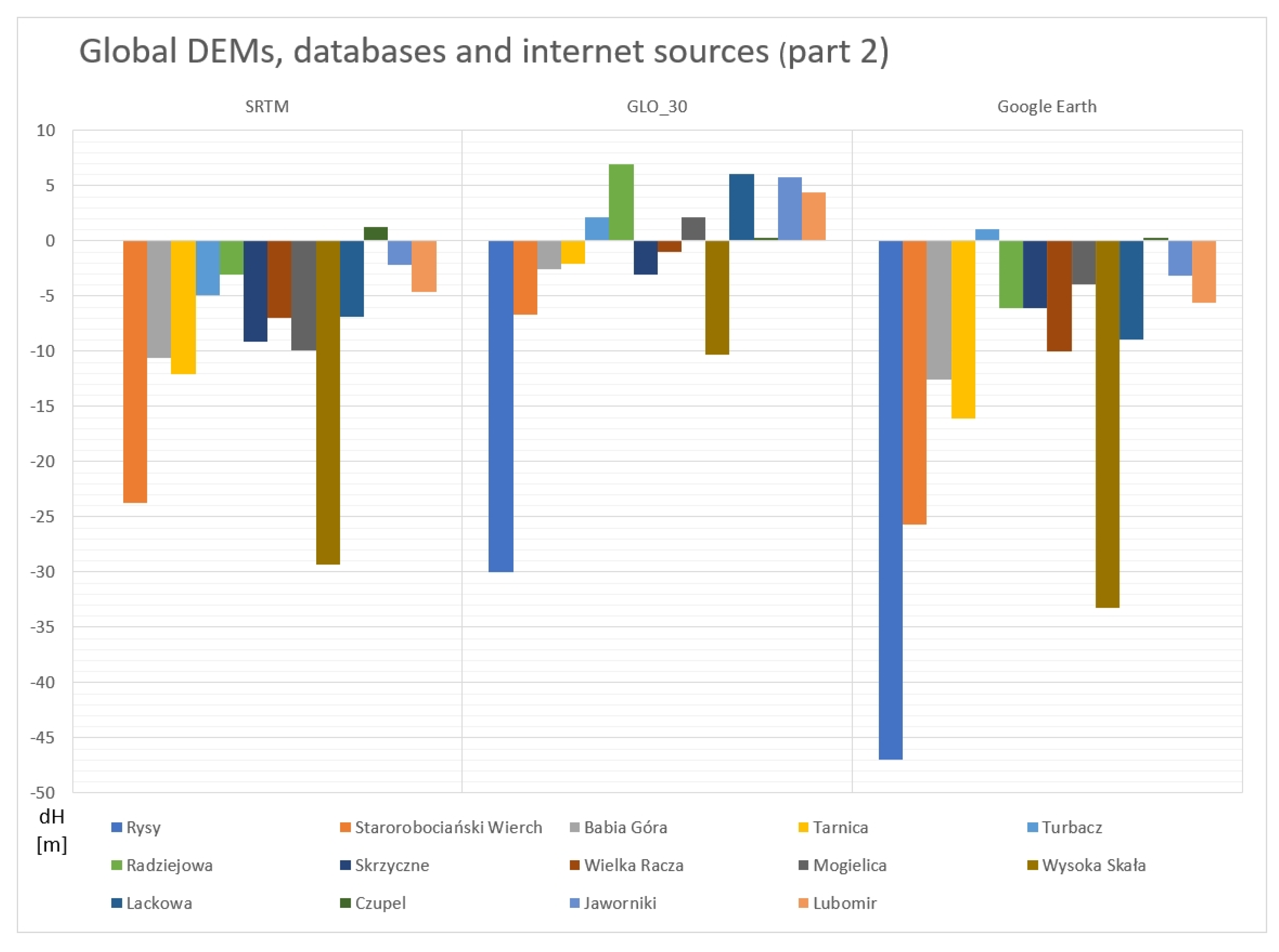
2.6. Global DEMs, Databases, and Internet Sources
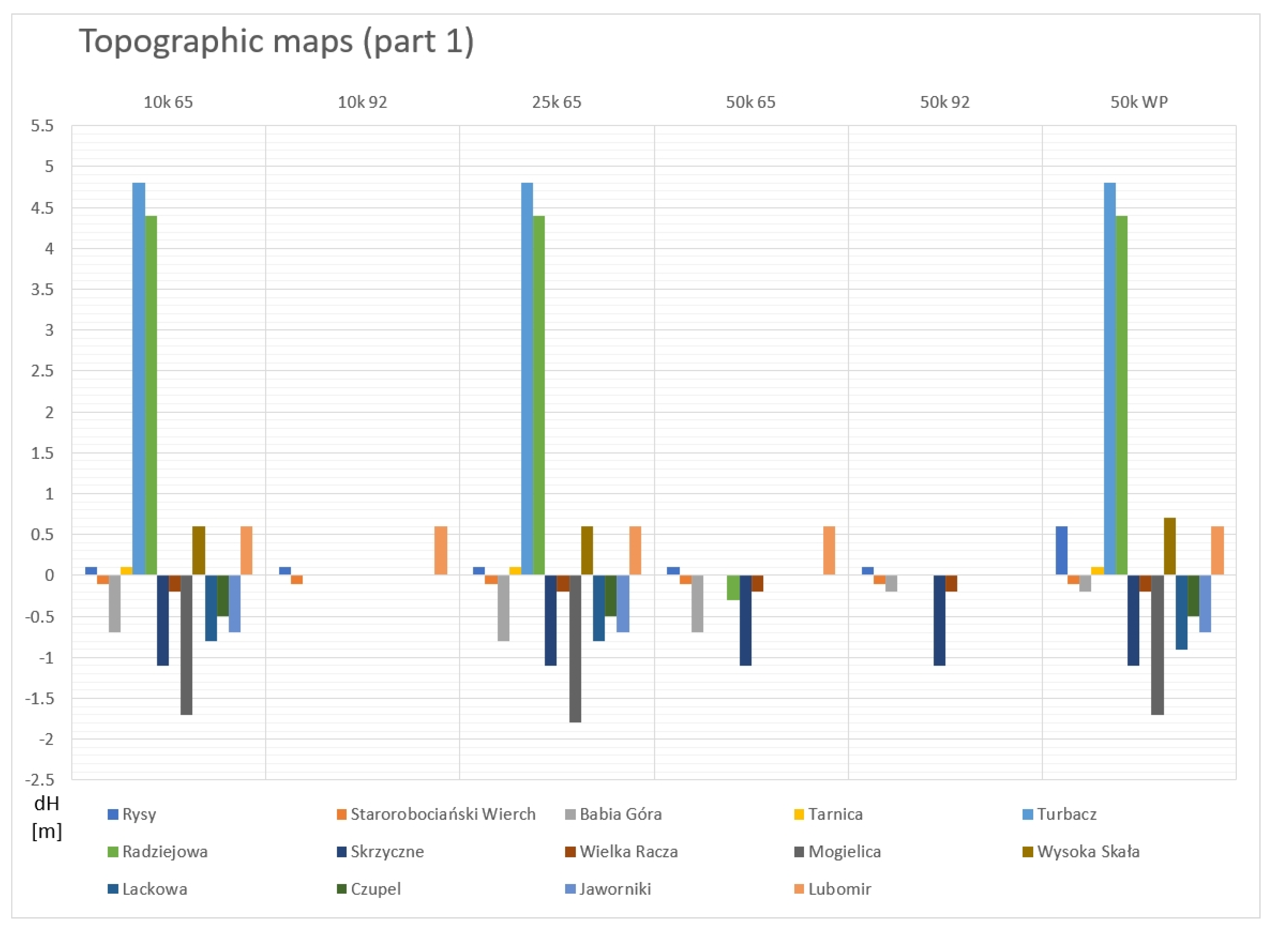
2.7. Polish Civil and Military Topographic Maps
- 1:10,000 in the PUWG 1965 coordinate system (10k 65)—civilian, (The abbreviation of the map series used in Appendix A is given in brackets)
- 1:10,000 in the PL-1992 (10k 92)—civilian,
- 1:25,000 in the PUWG 1965 (25k 65)—civilian,
- 1:50,000 in the PUWG 1965 (50k 65)—civilian,
- 1:50,000 in the PL-1992 (50k 92)—civilian,
- 1:50,000 in the UTM (50k WP)—military,
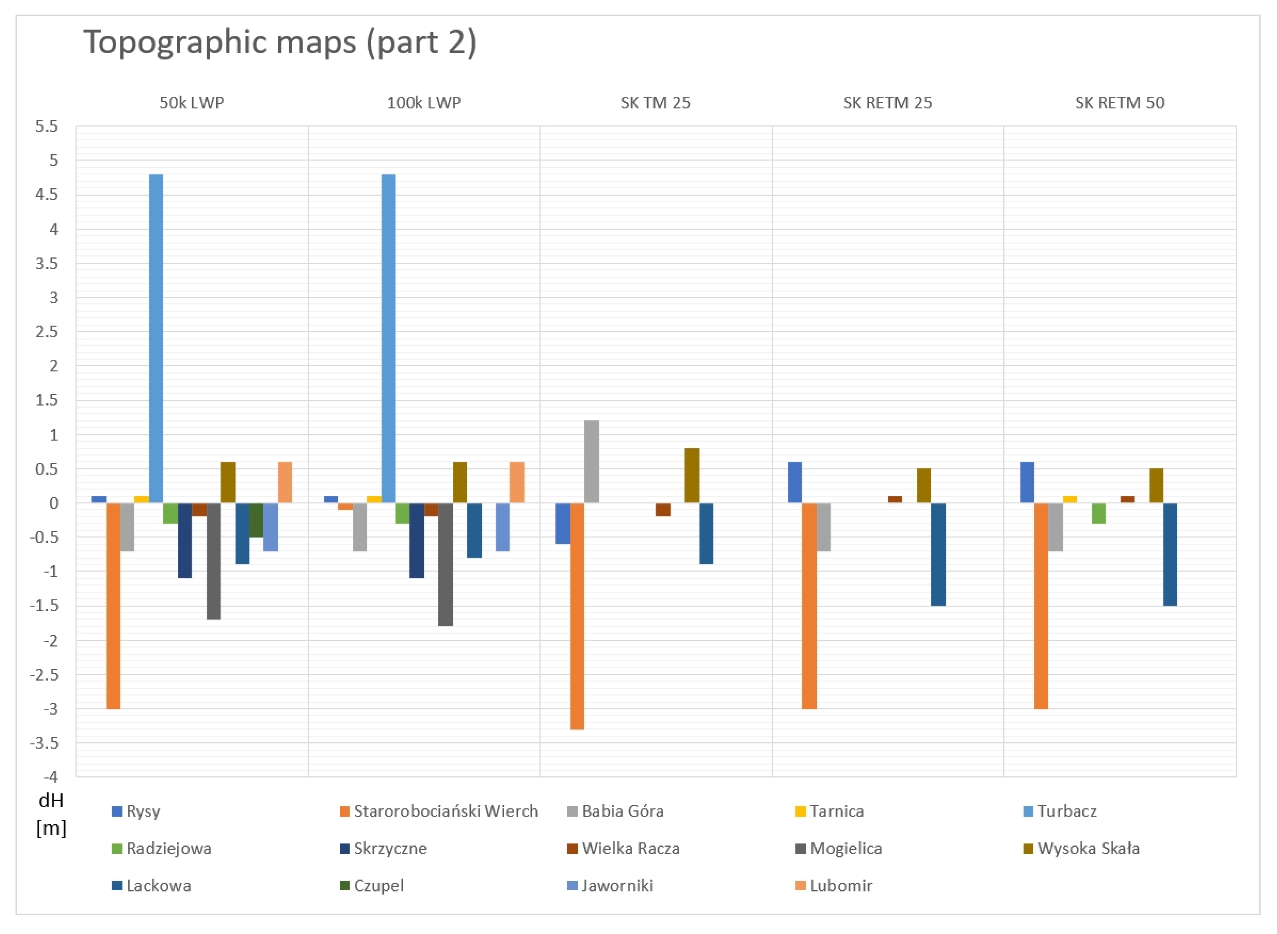
- 1:50,000 in the PUWG 1942 (50k LWP)—military,
- 1:100,000 in the PUWG 1942 (100k LWP)—military-civilian.
2.8. Slovak Civil and Military Topographic Maps
2.9. Books and Small-Scale Map Sources
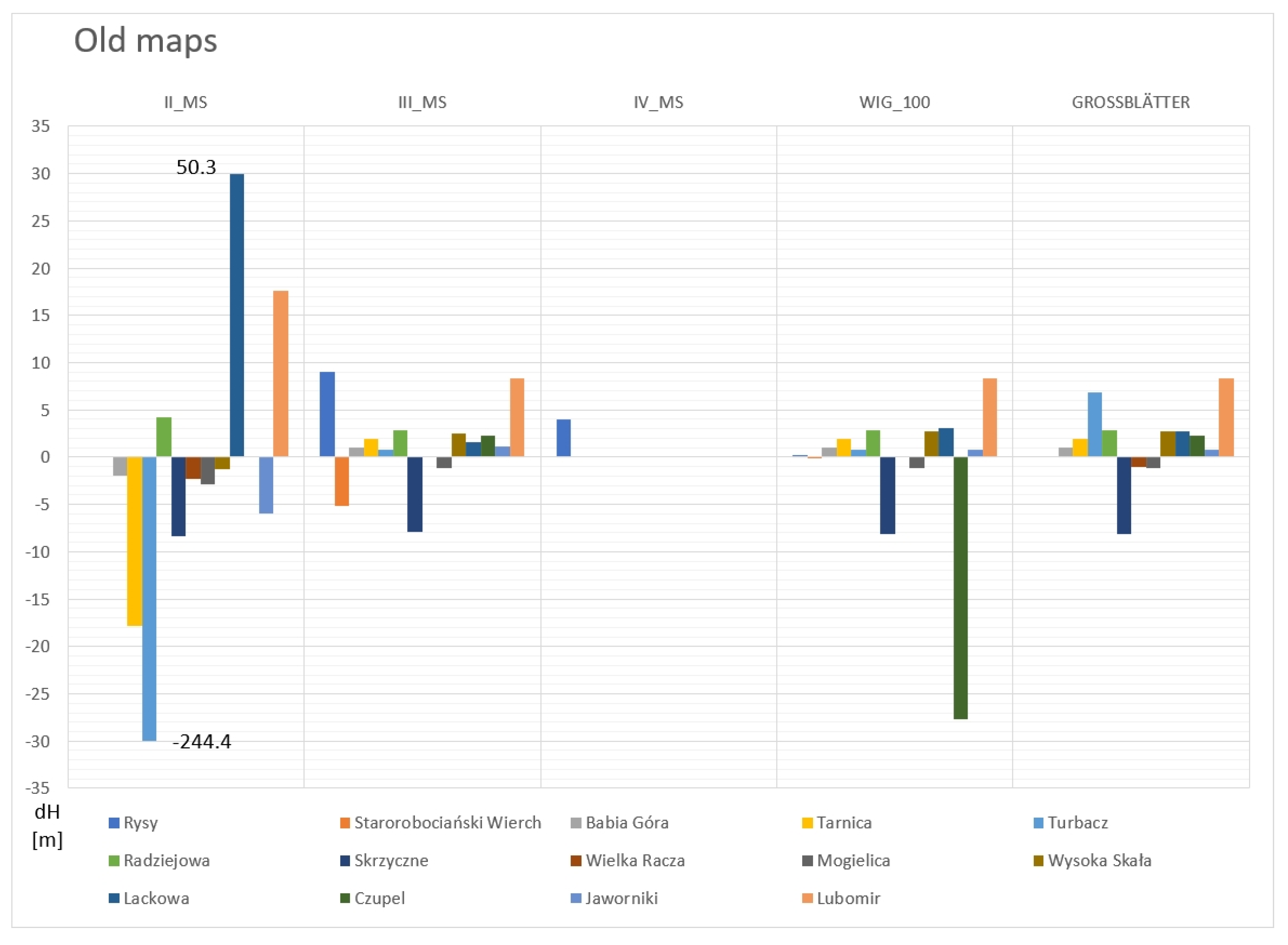
2.10. Old Maps
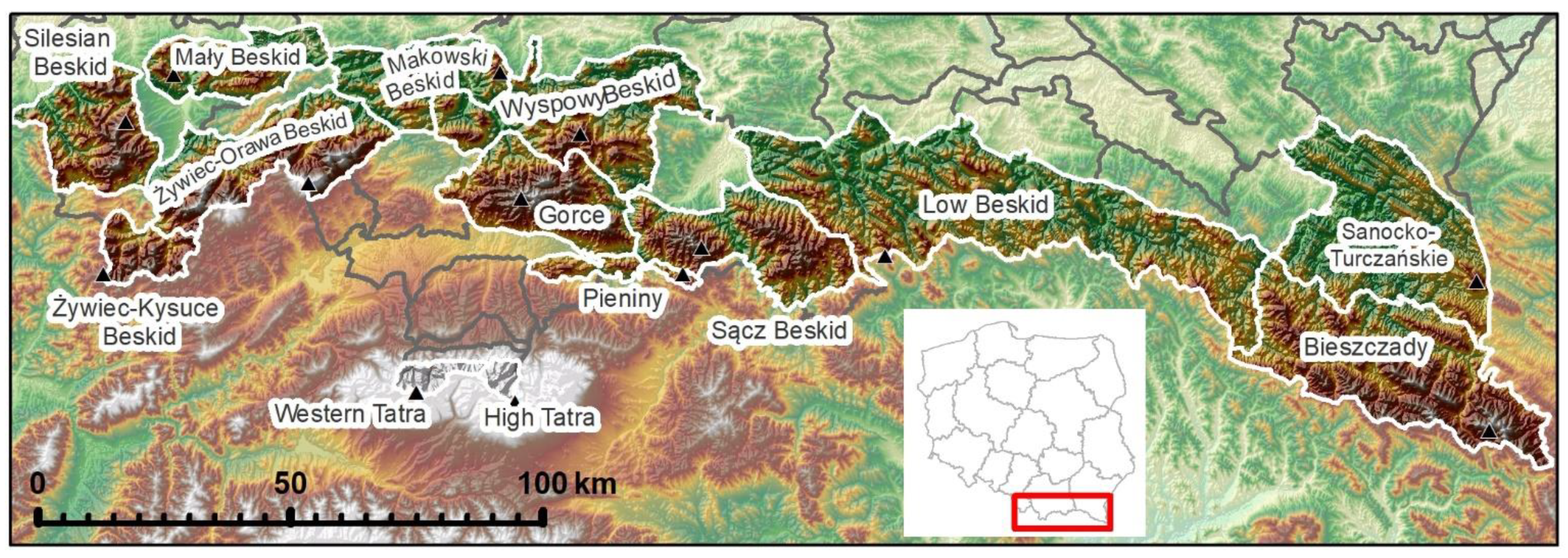
2.11. Study Area
3. Results
3.1. GNSS—Geodetic
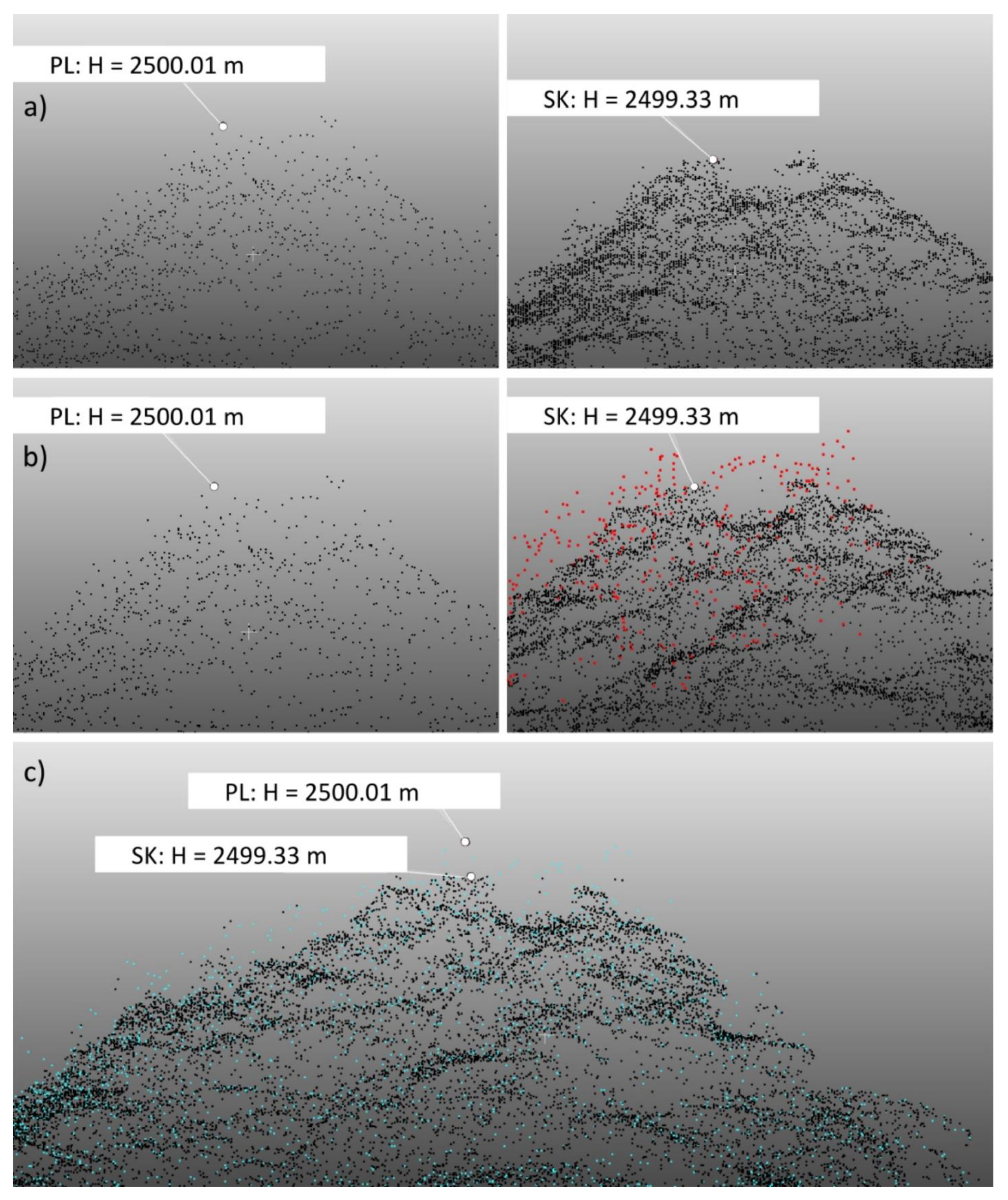
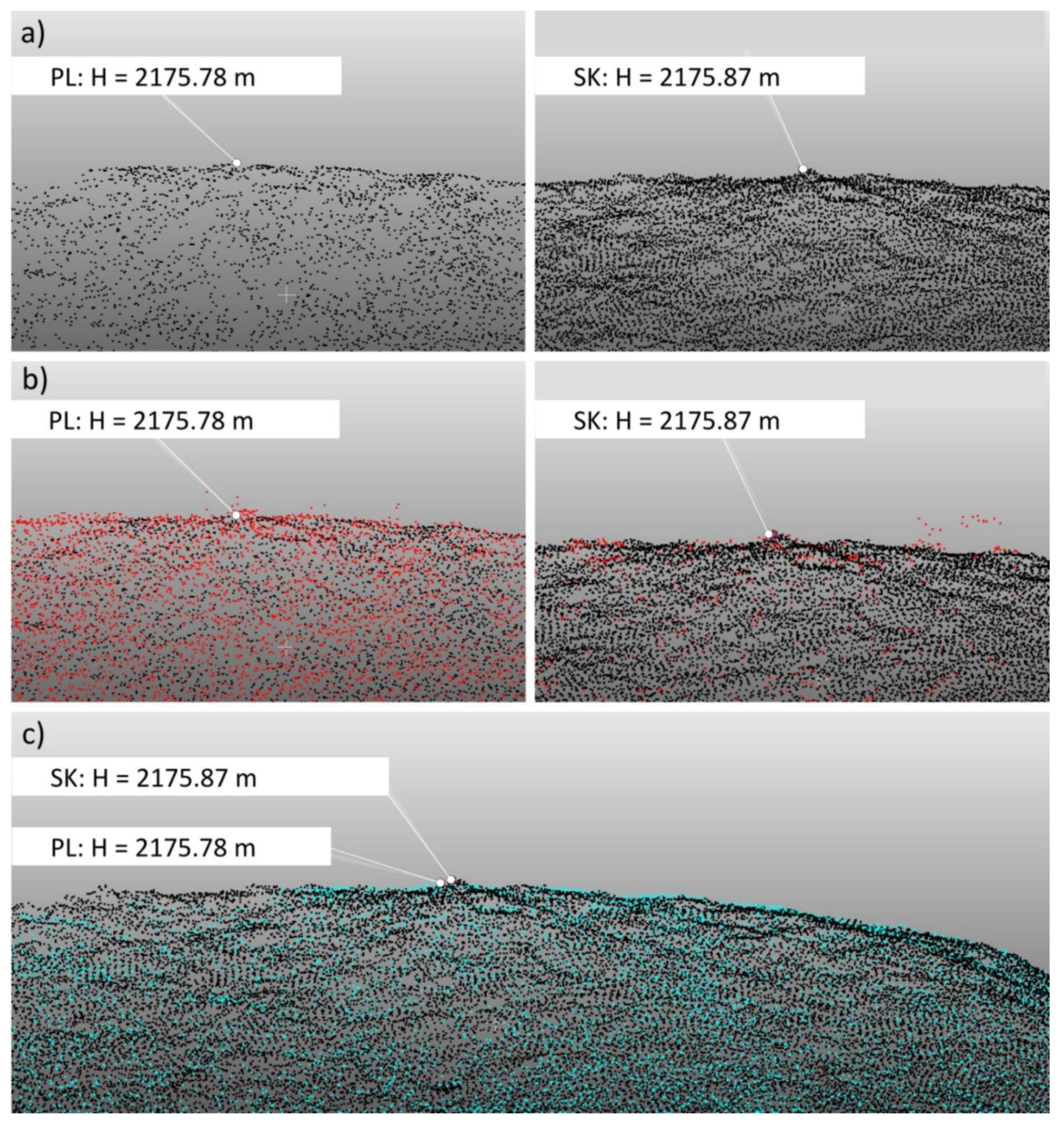
3.2. Slovak LiDAR—Analyses
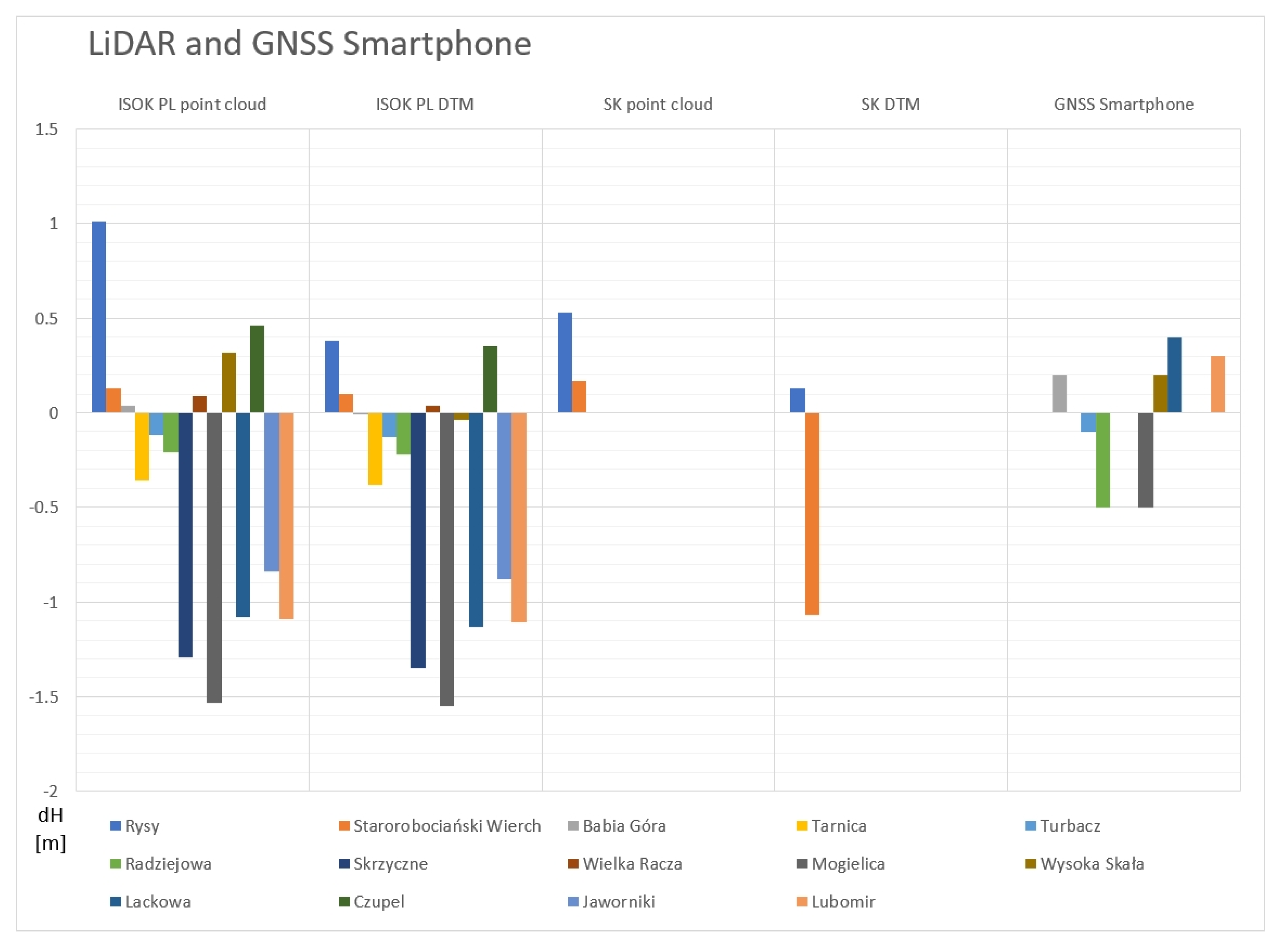
3.3. Polish LiDAR—Analyses
3.4. Slovak and Polish LiDAR—Comparison
3.5. Smartphone GNSS Measurements
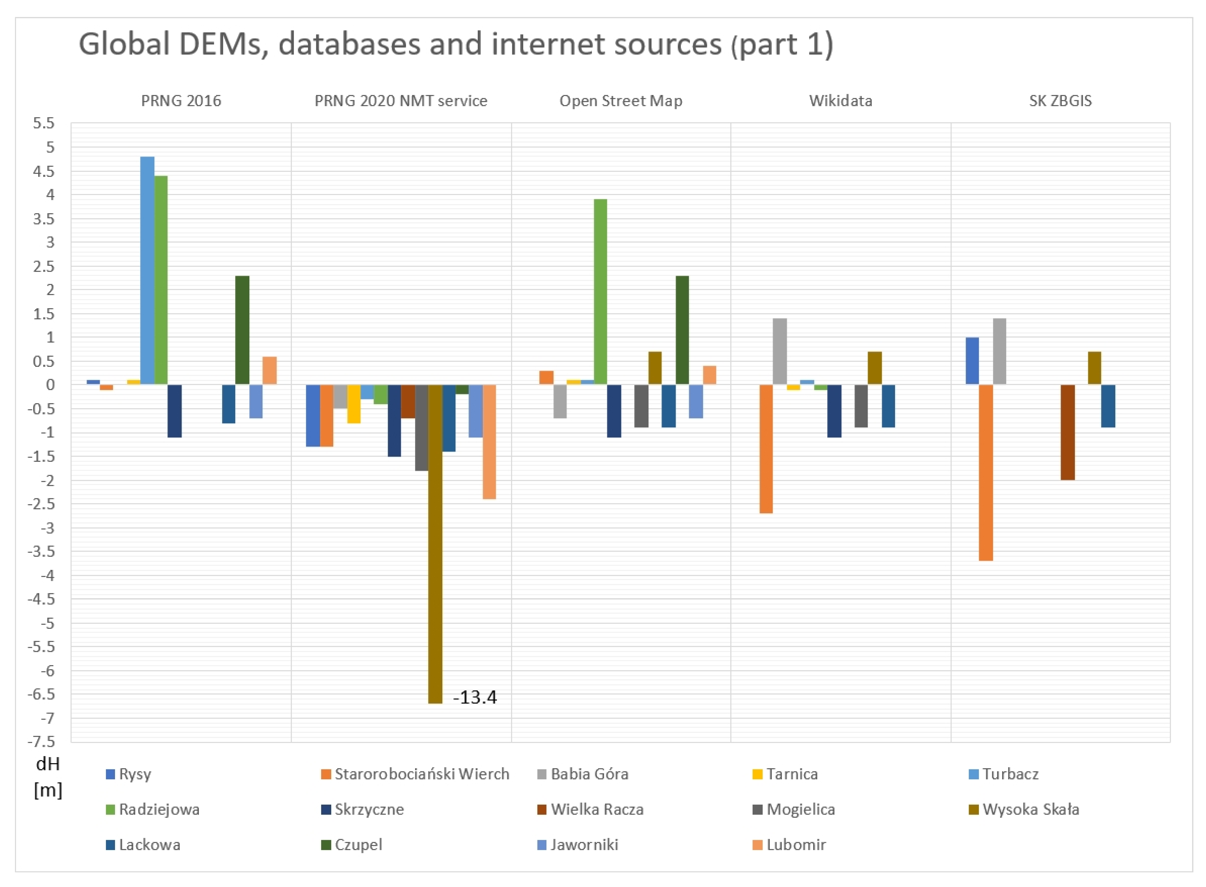
3.6. Global DEMs, Databases, and Internet Sources
3.7. Civilian and Military Topographic Maps (Polish and Slovak)
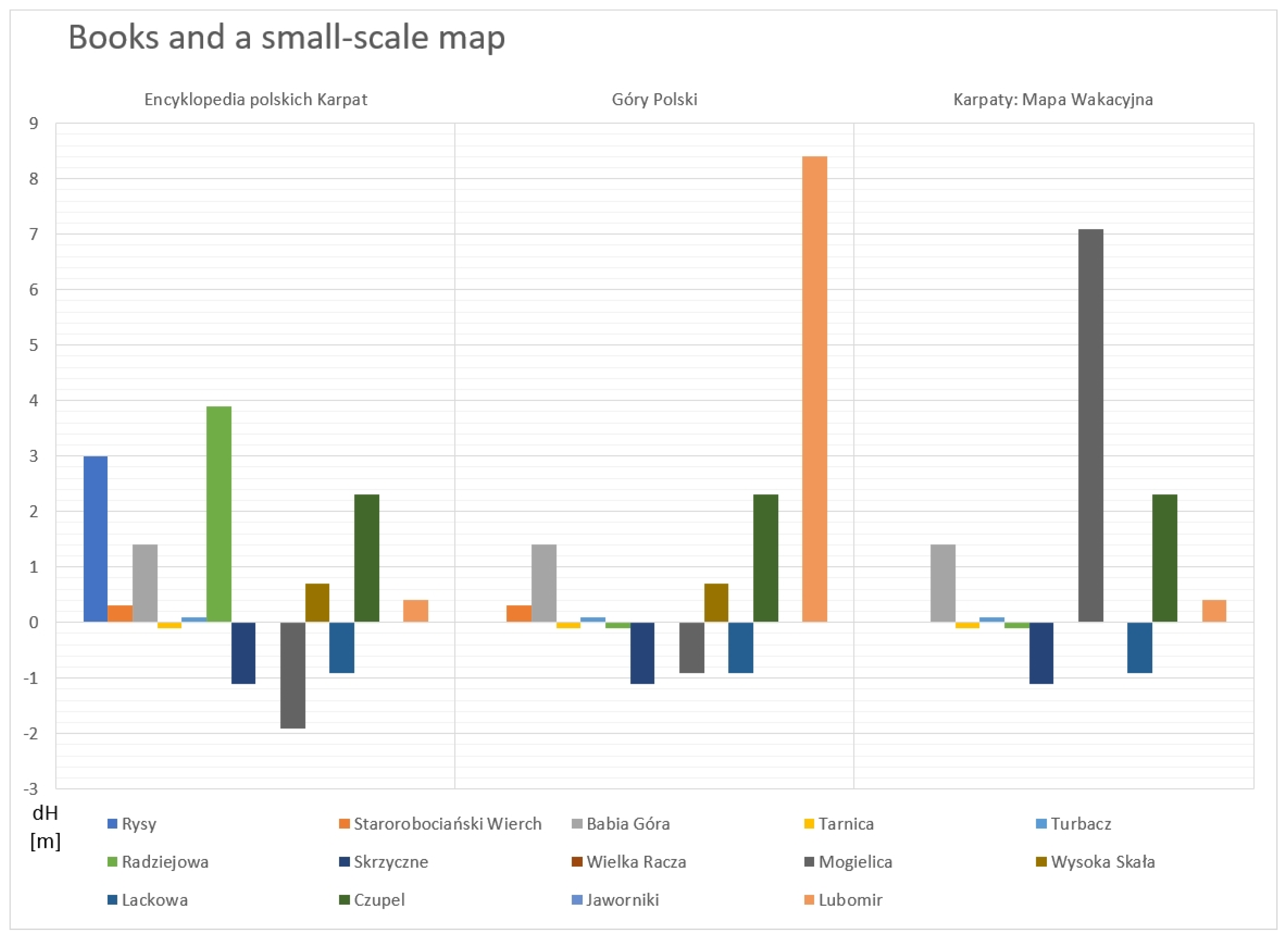
3.8. Books and Small-Scale Map Sources
3.9. Old Maps
4. Discussion
5. Conclusions
Author Contributions
Funding
Institutional Review Board Statement
Informed Consent Statement
Data Availability Statement
Acknowledgments
Conflicts of Interest
Appendix A

| No | Summit | GNSSMeasurement | ISOK PL Point Cloud | ISOK PL DTM | SK Point Cloud | SK DTM | GNSS Smartphone | SRTM | GLO_30 | |
| (1) | (2) | (3) | (4) | (5) | (6) | (7) | (8) | |||
| 1 | Rysy | 2499.0 | 2500.01 | 2499.38 | 2499.53 | 2499.13 | 2469 | |||
| 2 | Starorobociański Wierch | 2175.7 | 2175.83 | 2175.80 | 2175.87 | 2174.63 | 2152 | 2169 | ||
| 3 | Babia Góra | 1723.6 | 1723.64 | 1723.59 | 1723.80 | 1713 | 1721 | |||
| 4 | Tarnica | 1346.1 | 1345.74 | 1345.72 | 1334 | 1344 | ||||
| 5 | Turbacz | 1309.9 | 1309.78 | 1309.77 | 1309.80 | 1305 | 1312 | |||
| 6 | Radziejowa | 1262.1 | 1261.89 | 1261.88 | 1261.60 | 1259 | 1269 | |||
| 7 | Skrzyczne | 1258.1 | 1256.81 | 1256.75 | 1249 | 1255 | ||||
| 8 | Wielka Racza | 1236.0 | 1236.09 | 1236.04 | 1229 | 1235 | ||||
| 9 | Mogielica | 1171.9 | 1170.37 | 1170.35 | 1171.40 | 1162 | 1174 | |||
| 10 | Wysoka Skała | 1049.3 | 1049.62 | 1049.26 | 1049.50 | 1020 | 1039 | |||
| 11 | Lackowa | 997.9 | 996.82 | 996.77 | 998.30 | 991 | 1004 | |||
| 12 | Czupel | 930.7 | 931.16 | 931.05 | 930.70 | 932 | 931 | |||
| 13 | Jaworniki | 909.2 | 908.36 | 908.32 | 907 | 915 | ||||
| 14 | Lubomir | 903.6 | 902.51 | 902.49 | 903.90 | 899 | 908 | |||
| No | Summit | Google Earth | PRNG 2016 | PNRG 2020 NMT Service | Open Street Map | Wikidata | SK ZBGIS | 10k 65 | 10k 92 | |
| (9) | (10) | (11) | (12) | (13) | (14) | (15) | (16) | |||
| 1 | Rysy | 2452 | 2499.1 | 2497.7 | 2499 | 2499 | 2500 | 2499.1 | 2499.1 | |
| 2 | Starorobociański Wierch | 2150 | 2175.6 | 2174.4 | 2176 | 2173 | 2172 | 2175.6 | 2175.6 | |
| 3 | Babia Góra | 1711 | 1723.1 | 1722.9 | 1725 | 1725 | 1722.9 | |||
| 4 | Tarnica | 1330 | 1346.2 | 1345.3 | 1346.2 | 1346 | 1346.2 | |||
| 5 | Turbacz | 1311 | 1314.7 | 1309.6 | 1310 | 1310 | 1314.7 | |||
| 6 | Radziejowa | 1256 | 1266.5 | 1261.7 | 1266 | 1262 | 1266.5 | |||
| 7 | Skrzyczne | 1252 | 1257.0 | 1256.6 | 1257 | 1257 | 1257 | |||
| 8 | Wielka Racza | 1226 | 1236.0 | 1235.3 | 1236 | 1236 | 1234 | 1235.8 | ||
| 9 | Mogielica | 1168 | 1170.1 | 1171 | 1171 | 1170.2 | ||||
| 10 | Wysoka Skała | 1016 | 1035.9 | 1050 | 1050 | 1050 | 1049.9 | |||
| 11 | Lackowa | 989 | 997.1 | 996.5 | 997 | 997 | 997 | 997.1 | ||
| 12 | Czupel | 931 | 933.0 | 930.5 | 933 | 930.2 | ||||
| 13 | Jaworniki | 906 | 908.5 | 908.1 | 908.5 | 908.5 | ||||
| 14 | Lubomir | 898 | 904.2 | 901.2 | 904 | 904.2 | 904.2 | |||
| No | Summit | 25k 65 | 50k 65 | 50k 92 | 50k WP | 50k LWP | 100k LWP | SK TM 25 | SK RETM 25 | |
| (17) | (18) | (19) | (20) | (21) | (22) | (23) | (24) | |||
| 1 | Rysy | 2499.1 | 2499.1 | 2499.1 | 2499.6 | 2499.1 | 2499.1 | 2498.4 | 2499.6 | |
| 2 | Starorobociański Wierch | 2175.6 | 2175.6 | 2175.6 | 2175.6 | 2172.7 | 2175.6 | 2172.4 | 2172.7 | |
| 3 | Babia Góra | 1722.8 | 1722.9 | 1723.4 | 1723.4 | 1722.9 | 1722.9 | 1724.8 | 1722.9 | |
| 4 | Tarnica | 1346.2 | 1346.2 | 1346.2 | 1346.2 | |||||
| 5 | Turbacz | 1314.7 | 1314.7 | 1314.7 | 1314.7 | |||||
| 6 | Radziejowa | 1266.5 | 1261.8 | 1266.5 | 1261.8 | 1261.8 | ||||
| 7 | Skrzyczne | 1257 | 1257 | 1257 | 1257 | 1257 | 1257 | |||
| 8 | Wielka Racza | 1235.8 | 1235.8 | 1235.8 | 1235.8 | 1235.8 | 1235.8 | 1235.8 | 1236.1 | |
| 9 | Mogielica | 1170.1 | 1170.2 | 1170.2 | 1170.1 | |||||
| 10 | Wysoka Skała | 1049.9 | 1050 | 1049.9 | 1049.9 | 1050.1 | 1049.8 | |||
| 11 | Lackowa | 997.1 | 997 | 997 | 997.1 | 997 | 996.4 | |||
| 12 | Czupel | 930.2 | 930.2 | 930.2 | 898.8 | |||||
| 13 | Jaworniki | 908.5 | 908.5 | 908.5 | 908.5 | |||||
| 14 | Lubomir | 904.2 | 904.2 | 904.2 | 904.2 | 904.2 | ||||
| No | Summit | SK RETM 50 | Encyklopedia Polskich Karpat | Góry Polski | Karpaty: Mapa Wakacyjna | II_MS | III_MS | IV_MS | WIG_100 | GROSSBLÄTTER |
| (25) | (26) | (27) | (28) | (29) | (30) | (31) | (32) | (33) | ||
| 1 | Rysy | 2499.6 | 2502 | 2499 | 2499 | 2508 | 2503 | 2499.2 | ||
| 2 | Starorobociański Wierch | 2172.7 | 2176 | 2176 | 2170.6 | 2175.6 | ||||
| 3 | Babia Góra | 1722.9 | 1725 | 1725 | 1725 | 1721.7 | 1724.6 | 1724.6 | 1724.6 | |
| 4 | Tarnica | 1346.2 | 1346 | 1346 | 1346 | 1328.2 | 1348 | 1348 | 1348 | |
| 5 | Turbacz | 1310 | 1310 | 1310 | 1065.5 | 1310.7 | 1310.7 | 1316.7 | ||
| 6 | Radziejowa | 1261.8 | 1266 | 1262 | 1262 | 1266.3 | 1265 | 1265 | 1265 | |
| 7 | Skrzyczne | 1257 | 1257 | 1257 | 1249.7 | 1250.2 | 1250 | 1250 | ||
| 8 | Wielka Racza | 1236.1 | 1236 | 1236 | 1233.7 | 1236 | 1236 | 1235 | ||
| 9 | Mogielica | 1170 | 1171 | 1179 | 1169 | 1170.8 | 1170.8 | 1170.8 | ||
| 10 | Wysoka Skała | 1049.8 | 1050 | 1050 | 1048 | 1051.8 | 1052 | 1052 | ||
| 11 | Lackowa | 996.4 | 997 | 997 | 997 | 1048.2 | 999.5 | 1001 | 1000.6 | |
| 12 | Czupel | 933 | 933 | 933 | 933 | 903 | 933 | |||
| 13 | Jaworniki | 903.2 | 910.3 | 910 | 910 | |||||
| 14 | Lubomir | 904 | 912 | 904 | 883.3 (921.2) | 912 ? | 912 | 912 |
Appendix B


References
- Cajori, F. History of Determinations of the Heights of Mountains. Isis 1929, 12, 482–514. [Google Scholar] [CrossRef]
- Makowska, A. Precyzyjna niwelacja trygonometryczna w terenach górskich. Pr. Inst. Geod. Kartogr. 1986, 37, 193–220. [Google Scholar]
- Lambrecht, A.; Mayer, C.; Wendt, A.; Floricioiu, D.; Völksen, C. Elevation change of Fedchenko Glacier, Pamir Mountains, from GNSS field measurements and TanDEM-X elevation models, with a focus on the upper glacier. J. Glaciol. 2018, 64, 637–648. [Google Scholar] [CrossRef] [Green Version]
- Ching, K.E.; Hsieh, M.L.; Johnson, K.M.; Chen, K.H.; Rau, R.J.; Yang, M. Modern vertical deformation rates and mountain building in Taiwan from precise leveling and continuous GPS observations, 2000–2008. J. Geophys. Res. Solid Earth 2011, 116, 2000–2008. [Google Scholar] [CrossRef]
- Webster, T.L.; Dias, G. An automated GIS procedure for comparing GPS and proximal LIDAR elevations. Comput. Geosci. 2006, 32, 713–726. [Google Scholar] [CrossRef]
- Rieg, L.; Wichmann, V.; Rutzinger, M.; Sailer, R.; Geist, T.; Stötter, J. Data infrastructure for multitemporal airborne LiDAR point cloud analysis—Examples from physical geography in high mountain environments. Comput. Environ. Urban. Syst. 2014, 45, 137–146. [Google Scholar] [CrossRef]
- Xiong, L.; Wang, G.; Bao, Y.; Zhou, X.; Sun, X.; Zhao, R. Detectability of repeated airborne laser scanning for mountain landslide monitoring. Geoscience 2018, 8, 469. [Google Scholar] [CrossRef] [Green Version]
- Radebaugh, J.; Lorenz, R.D.; Kirk, R.L.; Lunine, J.I.; Stofan, E.R.; Lopes, R.M.C.; Wall, S.D. Mountains on Titan observed by Cassini Radar. Icarus 2007, 192, 77–91. [Google Scholar] [CrossRef]
- Germann, U.; Galli, G.; Boscacci, M.; Bolliger, M. Radar precipitation measurement in a mountainous region. Q. J. R. Meteorol. Soc. 2006, 132, 1669–1692. [Google Scholar] [CrossRef]
- Khanal, A.K.; Delrieu, G.; Cazenave, F.; Boudevillain, B. Radar remote sensing of precipitation in high mountains: Detection and characterization of melting layer in the grenoble valley, french Alps. Atmosphere 2019, 10, 784. [Google Scholar] [CrossRef] [Green Version]
- Hopkinson, C.; Hayashi, M.; Peddle, D. Comparing alpine watershed attributes from LiDAR, Photogrammetric, and Contour-based Digital Elevation Models. Hydrol. Process. 2009, 23, 451–463. [Google Scholar] [CrossRef]
- Müller, J.; Gärtner-Roer, I.; Thee, P.; Ginzler, C. Accuracy assessment of airborne photogrammetrically derived high-resolution digital elevation models in a high mountain environment. ISPRS J. Photogramm. Remote Sens. 2014, 98, 58–69. [Google Scholar] [CrossRef]
- Lewińska, P.; Dyczko, A. Thermal Digital Terrain Model of a Coal Spoil Tip—A Way of Improving Monitoring and Early Diagnostics of Potential Spontaneous Combustion Areas. J. Ecol. Eng. 2016, 17, 170–179. [Google Scholar] [CrossRef]
- Egholm, D.L.; Nielsen, S.B.; Pedersen, V.K.; Lesemann, J.E. Glacial effects limiting mountain height. Nature 2009, 460, 884–887. [Google Scholar] [CrossRef]
- Angus-Leppan, P.V. The height of mount everest. Surv. Rev. 1982, 26, 367–385. [Google Scholar] [CrossRef]
- Khadka, N.S. Mt Everest Grows by Nearly a Metre to New Height. Available online: https://www.bbc.com/news/world-asia-55218443 (accessed on 21 April 2021).
- Romanyshyn, I.; Hajdukiewicz, M. The Height Survey of Mount Łysica in The Context of Verification of Geodesical and Cartographic Studies. Struct. Environ. 2019, 11, 153–164. [Google Scholar] [CrossRef]
- Hajdukiewicz, M.; Romanyshyn, I. An accuracy assessment of spot heights on Digital Elevation Model (DEM) derived from ALS survey: Case study of Łysica massif. Struct. Environ. 2016, 9, 125–132. [Google Scholar]
- Kuraś, B. Spór o Wysokość Rysów. Mamy Szczyt Sięgający 2500 m n.p.m.? Available online: https://krakow.wyborcza.pl/krakow/7,174989,26240427,mamy-szczyt-siegajacy-2500-m-n-p-m.html?disableRedirects=true (accessed on 21 April 2021).
- Stäuble, S.; Martin, S.; Reynard, E. Historical Mapping for Landscape Reconstruction Historical Mapping for Landscape Reconstruction Examples from the Canton of Valais (Switzerland). In Proceedings of the 6th ICA Mountain Cartography Workshop, Mountain Mapping and Visualisation, ETH Zurich, Institute of Cartography, Lenk, Switzerland, 11–15 February 2008; pp. 211–217. [Google Scholar]
- Berczi, S. Reminiscent of an old book: “Critical review of minerals from Transylvania” by A. Koch, Kolozsvár, 1885: Proofs for the existence of anorthite-spinel-garnet peridotite series of inclusions in basalts of the Persányi Mountains Transylvania, Roumania. Acta Mineral. Petrogr. 1987, 29, 139–143. [Google Scholar]
- Migoń, P.; Kasprzak, M.; Traczyk, A. How high-resolution DEM based on airborne LiDAR helped to reinterpret landforms—Examples from the Sudetes, SW Poland. Landf. Anal. 2013, 22, 89–101. [Google Scholar] [CrossRef]
- Gu, C.; Clevers, J.G.P.W.; Liu, X.; Tian, X.; Li, Z.; Li, Z. Predicting forest height using the GOST, Landsat 7 ETM+, and airborne LiDAR for sloping terrains in the Greater Khingan Mountains of China. J. Photogramm. Remote Sens. 2018, 137, 97–111. [Google Scholar] [CrossRef]
- Hopkinson, C.; Demuth, M.N. Using airborne lidar to assess the influence of glacier downwasting on water resources in the Canadian Rocky Mountains. Can. J. Remote Sens. 2006, 32, 212–222. [Google Scholar] [CrossRef]
- Hyyppä, J.; Hyyppä, H.; Leckie, D.; Gougeon, F.; Yu, X.; Maltamo, M. Review of methods of small-footprint airborne laser scanning for extracting forest inventory data in boreal forests. Int. J. Remote Sens. 2008, 29, 1339–1366. [Google Scholar] [CrossRef]
- Baltsavias, E.P. Airborne Laser Scanning: Existing Systems and Firms and Other Resources. J. Photogramm. Remote Sens. 1999, 54, 164–198. [Google Scholar] [CrossRef]
- Estornell, J.; Ruiz, L.A.; Velázquez-Martí, B.; Hermosilla, T. Analysis of the factors affecting lidar dtm accuracy in a steep shrub area. Int. J. Digit. Earth 2011, 4, 521–538. [Google Scholar] [CrossRef] [Green Version]
- Simpson, J.E.; Smith, T.E.L.; Wooster, M.J. Assessment of errors caused by forest vegetation structure in airborne LiDAR-derived DTMs. Remote Sens. 2017, 9, 1101. [Google Scholar] [CrossRef] [Green Version]
- Kirmse, A.; de Ferranti, J. Calculating the prominence and isolation of every mountain in the world. Prog. Phys. Geogr. Earth Environ. 2017, 41, 788–802. [Google Scholar] [CrossRef]
- Schwarz, M.; Beul, M.; Droeschel, D.; Schüller, S.; Periyasamy, A.S.; Lenz, C.; Schreiber, M.; Behnke, S. Supervised autonomy for exploration and mobile manipulation in rough terrain with a centaur-like robot. Front. Robot. AI 2016, 3, 57. [Google Scholar] [CrossRef]
- Halme, A.; Leppänen, I.; Suomela, J.; Ylönen, S.; Kettunen, I. WorkPartner: Interactive human-like service robot for outdoor applications. Int. J. Rob. Res. 2003, 22, 627–640. [Google Scholar] [CrossRef]
- Zielinska, T. Professional and Personal Service Robots. Int. J. Robot. Appl. Technol. 2016, 4, 63–82. [Google Scholar] [CrossRef]
- Junyong, C.; Yanping, Z.; Janli, Y.; Chunxi, G.; Peng, Z. Height Determination of Qomolangma Feng (MT. Everest) in 2005. Surv. Rev. 2010, 42, 122–131. [Google Scholar] [CrossRef]
- Nishida, T.; Takemura, Y.; Fuchikawa, Y.; Kurogi, S.; Ito, S.; Obata, M.; Hiratsuka, N.; Miyagawa, H.; Watanabe, Y.; Suehiro, T.; et al. Development of a sensor system for outdoor service robot. In Proceedings of the 2006 SICE-ICASE International Joint Conference, Busan, Korea, 18–21 October 2006; Volume 10, pp. 2687–2691. [Google Scholar] [CrossRef] [Green Version]
- Raković, M.; Savić, S.; Santos-Victor, J.; Nikolić, M.; Borovac, B. Human-inspired online path planning and biped walking realization in unknown environment. Front. Neurorobot. 2019, 13, 36. [Google Scholar] [CrossRef]
- Sutherland, K.T.; Thompson, W.B. Localizing in Unstructured Environments: Dealing with the Errors. IEEE Trans. Robot. Autom. 1994, 10, 740–754. [Google Scholar] [CrossRef] [Green Version]
- Samala, N.; Katkam, B.S.; Bellamkonda, R.S.; Rodriguez, R.V. Impact of AI and robotics in the tourism sector: A critical insight. J. Tour. Futur. 2020. [Google Scholar] [CrossRef]
- Stankov, U.; Gretzel, U. Tourism 4.0 technologies and tourist experiences: A human-centered design perspective. Inf. Technol. Tour. 2020, 22, 477–488. [Google Scholar] [CrossRef]
- Yang, F.; Xue, X.; Cai, C.; Sun, Z.; Zhou, Q. Numerical simulation and analysis on spray drift movement of multirotor plant protection unmanned aerial vehicle. Energies 2018, 11, 2399. [Google Scholar] [CrossRef] [Green Version]
- Huang, H.; Savkin, A.V. Path planning for a solar-powered UAV inspecting mountain sites for safety and rescue. Energies 2021, 14, 1968. [Google Scholar] [CrossRef]
- Du, Y.C.; Zhang, M.X.; Ling, H.F.; Zheng, Y.J. Evolutionary Planning of Multi-UAV Search for Missing Tourists. IEEE Access 2019, 7, 73480–73492. [Google Scholar] [CrossRef]
- Lin, L.; Roscheck, M.; Goodrich, M.A.; Morse, B.S. Supporting Wilderness Search and Rescue with integrated intelligence: Autonomy and information at the right time and the right place. Proc. Natl. Conf. Artif. Intell. 2010, 3, 1542–1547. [Google Scholar]
- Caber, M.; Albayrak, T. Push or pull? Identifying rock climbing tourists’ motivations. Tour. Manag. 2016, 55, 74–84. [Google Scholar] [CrossRef]
- Burke, S.M.; Durand-Bush, N.; Doell, K. Exploring feel and motivation with recreational and elite Mount Everest climbers: An ethnographic study. Int. J. Sport Exerc. Psychol. 2010, 8, 373–393. [Google Scholar] [CrossRef]
- Apollo, M.; Mostowska, J.; Maciuk, K.; Wengel, Y.; Jones, T.E.; Cheer, J.M. Peak-bagging and cartographic misrepresentations: A call to correction. Curr. Issues Tour. 2021, 24, 1970–1975. [Google Scholar] [CrossRef]
- Lew, A.A.; Han, G. A world geography of mountain trekking. In Mountaineering Tourism; Routledge: London, UK, 2015; pp. 19–39. ISBN 9781317668732. [Google Scholar]
- Kuby, M.J.; Wentz, E.A.; Vogt, B.J.; Virden, R. Experiences in developing a tourism web site for hiking Arizona’s highest summits and deepest canyons. Tour. Geogr. 2001, 3, 454–473. [Google Scholar] [CrossRef]
- Crockett, L.J.; Murray, N.P.; Kime, D.B. Self-Determination Strategy in Mountaineering: Collecting Colorado’s Highest Peaks. Leis. Sci. 2020, 1–20. [Google Scholar] [CrossRef]
- Maciuk, K.; Apollo, M.; Cheer, J.M.; Konečný, O.; Kozioł, K.; Kudrys, J.; Mostowska, J.; Róg, M.; Skorupa, B.; Szombara, S. Determining Peak Altitude on Maps, Books and Cartographic Materials: Multidisciplinary Implications. Remote Sens. 2021, 13, 1111. [Google Scholar] [CrossRef]
- European Global Navigation Satellite System Agency. Using GNSS Raw Measurements on Android Devices; White Paper; Publications Office of the European Union: Luxembourg, 2017.
- Realini, E.; Caldera, S.; Pertusini, L.; Sampietro, D. Precise GNSS positioning using smart devices. Sensors 2017, 17, 2434. [Google Scholar] [CrossRef] [PubMed] [Green Version]
- Lachapelle, G.; Gratton, P.; Horrelt, J.; Lemieux, E.; Broumandan, A. Evaluation of a low cost hand held unit with GNSS raw data capability and comparison with an android smartphone. Sensors 2018, 18, 4185. [Google Scholar] [CrossRef] [PubMed] [Green Version]
- Natalia, W.; Tomasz, H. Czy to już możliwe? Geodeta 2019, 4, 8–12. [Google Scholar]
- Robustelli, U.; Baiocchi, V.; Pugliano, G. Assessment of dual frequency GNSS observations from a Xiaomi Mi 8 android smartphone and positioning performance analysis. Electronics 2019, 8, 91. [Google Scholar] [CrossRef] [Green Version]
- Wu, Q.; Sun, M.; Zhou, C.; Zhang, P. Precise Point Positioning Using Dual-Frequency. Sensors 2019, 19, 2189. [Google Scholar] [CrossRef] [Green Version]
- Uradziński, M.; Bakuła, M. Assessment of static positioning accuracy using low-cost smartphone GPS devices for geodetic survey points’ determination and monitoring. Appl. Sci. 2020, 10, 5308. [Google Scholar] [CrossRef]
- Gogoi, N.; Minetto, A.; Linty, N.; Dovis, F. A controlled-environment quality assessment of android GNSS raw measurements. Electronics 2019, 8, 5. [Google Scholar] [CrossRef] [Green Version]
- Mouratidis, A.; Ampatzidis, D. European digital elevation model validation against extensive global navigation satellite systems data and comparison with SRTM DEM and ASTER GDEM in Central Macedonia (Greece). Int. J. Geo-Inf. 2019, 8, 108. [Google Scholar] [CrossRef] [Green Version]
- Grochala, A.; Nerć, P. Ocena dokładności modelu SRTM 1 dla wybranych obszarów Polski. Przegląd Geodezyjny 2016, 1, 18–22. [Google Scholar] [CrossRef]
- Wężyk, P. (Ed.) Podręcznik dla Uczestników Szkoleń z Wykorzystania Produktów LiDAR, 2nd ed.; Główny Urząd Geodezji i Kartografii: Warszawa, Poland, 2015; ISBN 978-83-254-2100-7. [Google Scholar]
- Geodesy Cartography and Cadastre Authority of the Slovak Republic Mapový Klient ZBGIS. Available online: https://zbgis.skgeodesy.sk/mkzbgis/sk/teren (accessed on 23 January 2021).
- Geodesy Cartography and Cadastre Authority of the Slovak Republic Projekt—Digitálny Model Reliéfu. Available online: https://www.geoportal.sk/sk/udaje/lls-dmr/o-projekte/ (accessed on 23 January 2021).
- Geodesy Cartography and Cadastre Authority of the Slovak Republic Parametre pre Lokality Zberu Údajov LLS. Available online: https://www.geoportal.sk/files/zbgis/lls/parametre-lokality-zberu-udajov-lls.pdf (accessed on 23 January 2021).
- Geodesy Cartography and Cadastre Authority of the Slovak Republic Download. Available online: https://www.geoportal.sk/en/geodeticke-zaklady/download/ (accessed on 23 January 2021).
- Head Office of Geodesy and Cartography National Geoportal. Available online: https://mapy.geoportal.gov.pl/imap/Imgp_2.html (accessed on 12 February 2021).
- Geo++ RINEX Logger. Available online: https://play.google.com/store/apps/details?id=de.geopp.rinexlogger&hl=pl (accessed on 2 February 2021).
- RTKLIB: An Open Source Program Package for GNSS Positioning. Available online: http://www.rtklib.com/ (accessed on 2 February 2021).
- Rodríguez, E.; Morris, C.S.; Belz, J.E. A global assessment of the SRTM performance. Photogramm. Eng. Remote Sens. 2006, 72, 249–260. [Google Scholar] [CrossRef] [Green Version]
- Fahrland, E. Copernicus DEM Product Handbook (v3.0); Airbus Defence and Space GmbH: Taufkirchen, Germany, 2020. [Google Scholar]
- Lewandowicz, E. Evaluation of geographical potential of the Warmia and Mazury Province based on the National Register of Geographical Names using geoinformation tools. Ann. Geomat. 2016, XIV, 583–595. [Google Scholar]
- ZBGIS. Available online: https://www.geoportal.sk/en/zbgis/ (accessed on 25 February 2021).
- Stankiewicz, M. Zarys historii produkcji polskich urzędowych map topograficznych. In Rola Bazy Danych Obiektów Topograficznych w Tworzeniu Infrastruktury Informacji Przestrzennej w Polsce; Olszewski, R., Gotlib, D., Eds.; Główny Urząd Geodezji i Kartografii: Warszawa, Poland, 2013; pp. 26–33. ISBN 978-83-254-1975-2. [Google Scholar]
- Jakubík, J. Vývoj vojenskej kartografie na území slovenska. Kartografické Listy 2012, 20, 28–38. [Google Scholar]
- Zeman, M. Staré mapové diela na slovensku a ich publikovanie na internete. Kartografické Listy 2012, 20, 55–61. [Google Scholar]
- Malarz, R. Encyklopedia Karpat Polskich; Wydawnictwo Attyka: Kraków, Poland, 2020; ISBN 978-83-65644-73-2. [Google Scholar]
- Kluszczyński, R. Góry Polski—Przewodnik; Kluszczyński: Kraków, Poland, 2006; ISBN 83-7447-041-0. [Google Scholar]
- Sikorska, K.; Mikułowski, B.; Werner, Z. Karpaty: Mapa Wakacyjna 1:250,000; Polskie Przedsiębiorstwo Wydawnictw Kartograficznych im. Eugeniusza Romera (PPWK): Warszawa-Wrocław, Poland, 1998. [Google Scholar]
- Ostafin, K.; Kaim, D.; Troll, M.; Maciejowski, W. The authorship of the Second Military Survey of Galicia and Austrian Silesia at the scale 1:28,800 and the consistency of sheet content based on selected examples. Pol. Cartogr. Rev. 2020, 52, 141–151. [Google Scholar] [CrossRef]
- Timár, G. System of the 1:28 800 scale sheets of the Second Military Survey in Tyrol and Salzburg. Acta Geod. Geophys. Hung. 2009, 44, 95–104. [Google Scholar] [CrossRef] [Green Version]
- Křovák, J. Geodetické základy polohopisné a jednotný zobrazovací způsob Československé republiky. Zeměměřický Věstník 1938, 4, 54–58. [Google Scholar]
- Marek, J. Mapovanie—Historický Prehľad; Slovenská Spoločnosť Geodetov a Kartografov: Bratislava, Slovakia, 2007; ISBN 978-80-969692-1-0. [Google Scholar]
- Kuna, J. ‘Partially compiled’ maps 1:25,000 by Polish Military Geographical Institute (1919–1939). Pol. Cartogr. Rev. 2018, 50, 31–46. [Google Scholar] [CrossRef] [Green Version]
- Lewandowski, W.; Więckowski, M. Korona Gór Polski. Poznaj Swój Kraj 1997, XL, 17. [Google Scholar]
- Zarząd_Główny_PTTK; Kmisja_Turystyki_Górskiej_PTTK; Komisja_Turystyki_Narciarskiej. Górska Odznaka Turystyczna PTTK, Odznaki Narciarskie PTTK; Centralny Ośrodek Turystyki Górskiej PTTK: Kraków, Poland, 2015; ISBN 978-83-62473-59-5. [Google Scholar]
- Solon, J.; Borzyszkowski, J.; Bidłasik, M.; Richling, A.; Badora, K.; Balon, J.; Brzezińska-Wójcik, T.; Chabudziński, Ł.; Dobrowolski, R.; Grzegorczyk, I.; et al. Physico-geographical mesoregions of poland: Verification and adjustment of boundaries on the basis of contemporary spatial data. Geogr. Pol. 2018, 91, 143–170. [Google Scholar] [CrossRef]
- Bónová, K.; Bóna, J.; Pańczyk, M.; Kováčik, M.; Mikuš, T.; Laurinc, D. Origin of deep-sea clastics of the Magura Basin (Eocene Makovica sandstones in the Outer Western Carpathians) with constraints of framework petrography, heavy mineral analysis and zircon geochronology. Palaeogeogr. Palaeoclimat. Palaeoecol. 2019, 514, 768–784. [Google Scholar] [CrossRef]
- Pánek, T.; Minár, J.; Vitovič, L.; Břežný, M. Post-LGM faulting in Central Europe: LiDAR detection of the >50 km-long Sub-Tatra fault, Western Carpathians. Geomorphology 2020, 364, 107248. [Google Scholar] [CrossRef]
- Kozak, J. Forest Cover Changes and Their Drivers in the Polish Carpathian Mountains Since 1800. In Reforesting Landscapes; Nagendra, H., Southworth, J., Eds.; Springer: Dordrecht, The Netherlands, 2009; pp. 253–273. [Google Scholar]
- Siwicki, M. Nowe Ustalenia Dotyczące Wysokości Szczytów w Tatrach. Available online: https://geoforum.pl/news/29549/nowe-ustalenia-dotyczace-wysokosci-szczytow-w-tatrach (accessed on 2 September 2020).
- Pelc-Mieczkowska, R. Preliminary Analysis of the Applicability of the GPS PPP Method in Geodynamic Studies. Geomat. Environ. Eng. 2020, 14, 57–68. [Google Scholar] [CrossRef]
- Scalco, P.A.P.; Iescheck, A.L.; Corrêa, I.C.S.; Scottá, F.C.; de Oliveira, R.M.; Franchini, R.A.L. Validation of the Digital Elevation Model (SRTM) with GNSS Surveying Applied to the Mirim Lagoon Hydrographic Basin. Bol. Ciências Geodésicas 2018, 24, 407–425. [Google Scholar] [CrossRef]


| 513 | Outer Western Carpathians | 514-15 | Central Western Carpathians |
| 513.4-5 | Western Beskidy Mts | 514.1 | Orawa-Podhale Basin |
| 513.45 | Silesian Beskid Mts | 514.12 | Pieniny Mts |
| 513.47 | Mały Beskid Mts | 514.5 | Tatra Range |
| 513.48 | Makowski Beskid Mts | 514.52 | Western Tatra Mts |
| 513.49 | Wyspowy Beskid Mts | 514.53 | High Tatra Mts |
| 513.51 | Żywiec-Orawa Beskid Mts | 522 | Outer Eastern Carpathians |
| 513.52 | Gorce Mts | 522.1 | Lesiste Beskidy Mts |
| 513.54 | Sącz Beskid Mts | 522.11 | Sanocko-Turczańskie Mts |
| 513.56 | Żywiec-Kysuce Beskid Mts | 522.12 | Bieszczady Mts |
| 513.7 | Mid-Beskidy Mts | ||
| 513.71 | Low Beskid Mts |
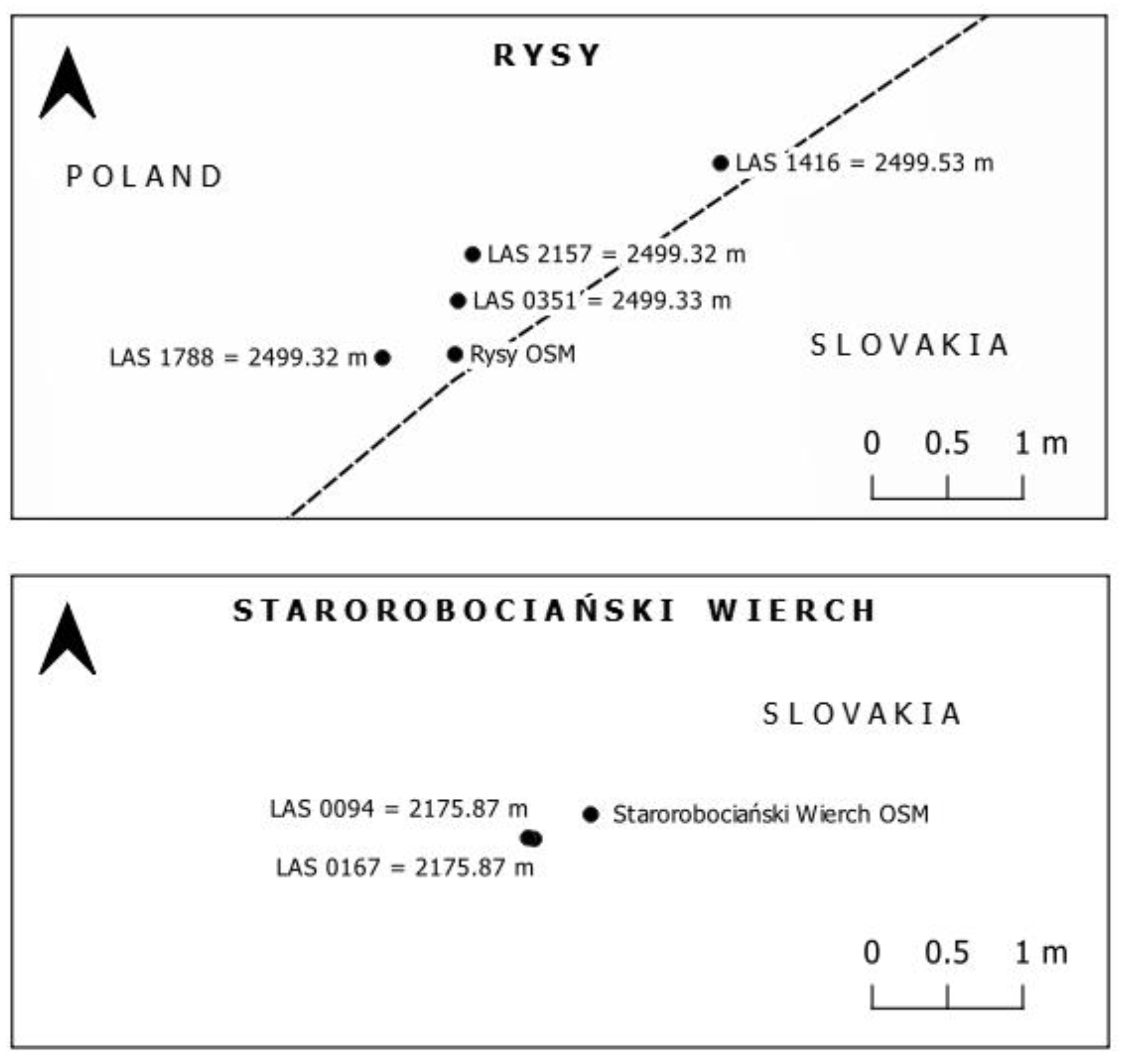
| Rysy | |||
|---|---|---|---|
| X PL-1992 [m] | Y PL-1992 [m] | H KRON86 [m] | |
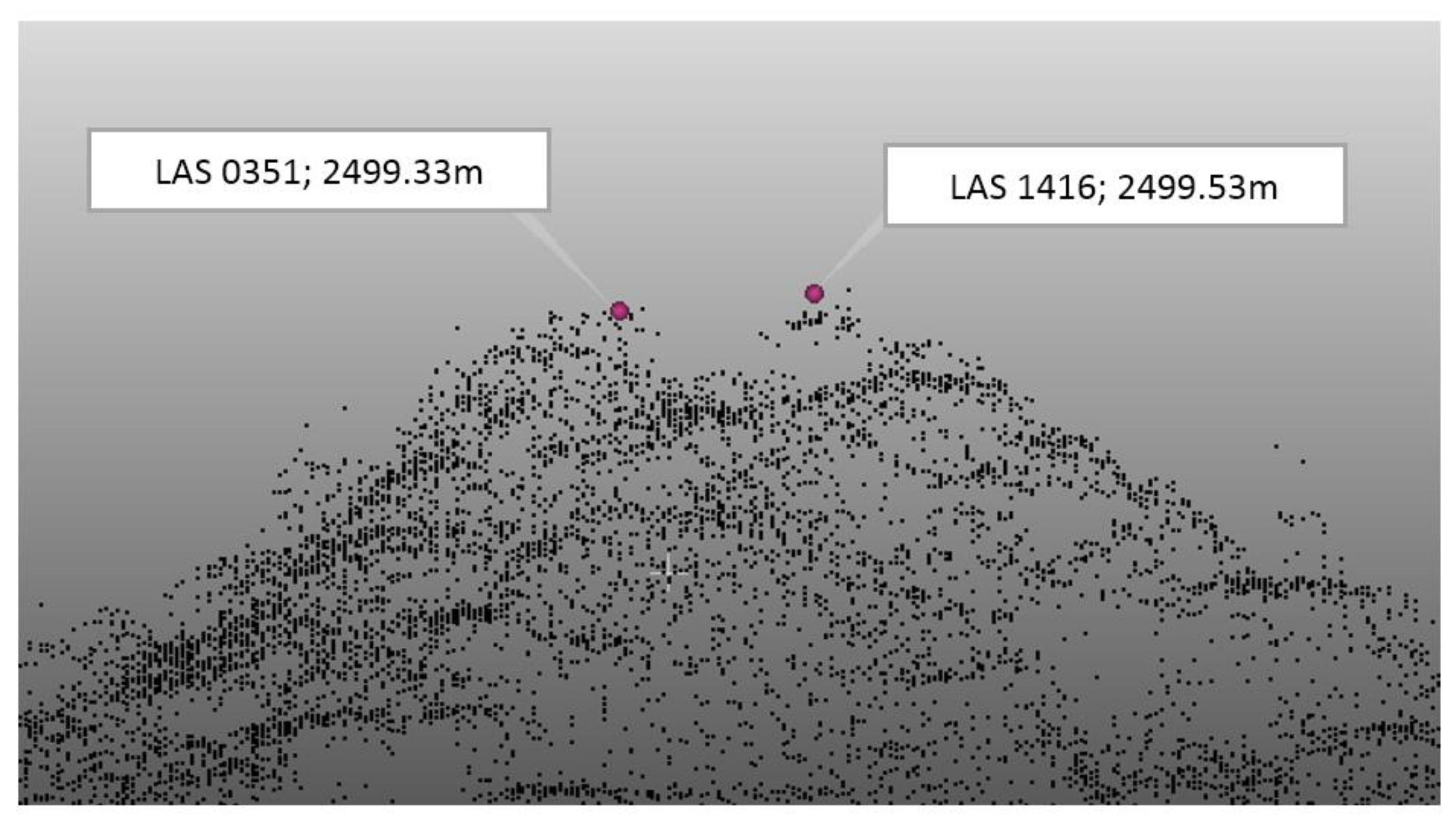
| LAS 1416 | 579273.31 | 146355.86 | 2499.53 |
| LAS 0351 | 579271.57 | 146354.95 | 2499.33 |
| LAS 1788 | 579271.07 | 146354.57 | 2499.32 |
| LAS 2157 | 579271.67 | 146355.26 | 2499.32 |
| Starorobociański Wierch | |||
| LAS 0094 | 559714.40 | 148307.06 | 2175.87 |
| LAS 0167 | 559714.44 | 148307.05 | 2175.87 |
| Peak | Dataset | Classification | Number of Points | The Highest [m] | Distance from the Peak [m] |
|---|---|---|---|---|---|
| RYSY | LAS 2157, Density = 8.93 pts/m2 | Ground | 26 | 2499.32 | 0.7 |
| Unclassified | 8 | 2500.15 | 0.1 | ||
| Total | 34 | - | - | ||
| LAS 1788, Density = 9.75 pts/m2 | Ground | 31 | 2499.32 | 0.5 | |
| Unclassified | 1 | 2499.34 | 0.3 | ||
| Total | 32 | - | - | ||
| LAS 0351, Density = 9.56 pts/m2 | Ground | 22 | 2499.33 | 0.4 | |
| Unclassified | 7 | 2500.17 | 0.3 | ||
| Medium vegetation | 2 | 2499.71 | 0.9 | ||
| Low vegetation | 1 | 2499.03 | 1 | ||
| Total | 32 | - | - | ||
| LAS 1416, Density = 7.96 pts/m2 | Ground | 14 | 2499.27 | 0.6 | |
| Unclassified | 10 | 2499.64 | 0.9 | ||
| Total | 24 | - | - | ||
| STAROROBOCIAŃSKI WIERCH | LAS 0094, Density = 6.18 pts/m2 | Ground | 24 | 2175.87 | 0.4 |
| Low vegetation | 3 | 2175.82 | 0.5 | ||
| Total | 27 | - | - | ||
| LAS 0167, Density = 6.60 pts/m2 | Ground | 28 | 2175.87 | 0.4 | |
| Low vegetation | 2 | 2175.79 | 0.5 | ||
| Total | 30 | - | - |
| Peak | X PL-1992 [m] | Y PL-1992 [m] | H KRON86 [m] | Distance from the Peak [m] |
|---|---|---|---|---|
| RYSY | 579,271.18 | 146,354.96 | 2500.01 | 0.5 |
| STAROROBOCIAŃSKI WIERCH | 559,711.60 | 148,310.39 | 2175.83 | 4.5 |
| STAROROBOCIAŃSKI WIERCH | 559,714.01 | 148,306.63 | 2175.78 | 1 |
| Peak | Dataset | Classification | Number of Points | The Highest [m] | Distance from the Peak [m] |
|---|---|---|---|---|---|
| RYSY | Density = 6.95 pts/m2 | Ground | 19 | 2500.01 | 0.5 |
| Total | 19 | - | - | ||
| STAROROBOCIAŃSKI WIERCH | Density = 7.62 pts/m2 | Ground | 7 | 2175.78 | 1 |
| Low vegetation | 20 | 2175.98 | 0.5 | ||
| Medium vegetation | 3 | 2175.92 | 0.5 | ||
| Never classified | 1 | 2175.40 | 0.8 | ||
| Total | 31 | - | - |
| RYSY | |||||
|---|---|---|---|---|---|
| Dataset | X PL-1992 [m] | Y PL-1992 [m] | H KRON-86 [m] | point cloud density [pts/m2] | number of Ground points within a 1 m radius |
| distance between points [m] | |||||
| SK | 579,271.57 | 146,354.95 | 2499.33 | 35.97 | 93 |
| PL | 579,271.18 | 146,354.96 | 2500.01 | 6.95 | 19 |
| 0.39 | |||||
| STAROROBOCIAŃSKI WIERCH | |||||
| SK | 559,714.44 | 148,307.05 | 2175.87 | 16.29 | 52 |
| PL | 559,714.01 | 148,306.63 | 2175.78 | 7.62 | 7 |
| 0.60 | |||||
| Peak | Mountain Range | HS [m] | dHS [m] |
|---|---|---|---|
| Babia Góra | Żywiec-Orawa Beskid Mts | 1723.8 | 0.2 |
| Lubomir | Makowski Beskid Mts | 903.9 | 0.3 |
| Czupel | Mały Beskid Mts | 930.7 | 0.0 |
| Lackowa | Low Beskid Mts | 998.3 | 0.4 |
| Radziejowa | Sącz Beskid Mts | 1261.6 | -0.5 |
| Mogielica | Wyspowy Beskid Mts | 1171.4 | -0.5 |
| Turbacz | Gorce Mts | 1309.8 | -0.1 |
| Wysoka Skała | Pieniny Mts | 1049.5 | 0.2 |
Publisher’s Note: MDPI stays neutral with regard to jurisdictional claims in published maps and institutional affiliations. |
© 2021 by the authors. Licensee MDPI, Basel, Switzerland. This article is an open access article distributed under the terms and conditions of the Creative Commons Attribution (CC BY) license (https://creativecommons.org/licenses/by/4.0/).
Share and Cite
Szombara, S.; Róg, M.; Kozioł, K.; Maciuk, K.; Skorupa, B.; Kudrys, J.; Lepeška, T.; Apollo, M. The Highest Peaks of the Mountains: Comparing the Use of GNSS, LiDAR Point Clouds, DTMs, Databases, Maps, and Historical Sources. Energies 2021, 14, 5731. https://doi.org/10.3390/en14185731
Szombara S, Róg M, Kozioł K, Maciuk K, Skorupa B, Kudrys J, Lepeška T, Apollo M. The Highest Peaks of the Mountains: Comparing the Use of GNSS, LiDAR Point Clouds, DTMs, Databases, Maps, and Historical Sources. Energies. 2021; 14(18):5731. https://doi.org/10.3390/en14185731
Chicago/Turabian StyleSzombara, Stanisław, Marta Róg, Krystian Kozioł, Kamil Maciuk, Bogdan Skorupa, Jacek Kudrys, Tomáš Lepeška, and Michal Apollo. 2021. "The Highest Peaks of the Mountains: Comparing the Use of GNSS, LiDAR Point Clouds, DTMs, Databases, Maps, and Historical Sources" Energies 14, no. 18: 5731. https://doi.org/10.3390/en14185731
APA StyleSzombara, S., Róg, M., Kozioł, K., Maciuk, K., Skorupa, B., Kudrys, J., Lepeška, T., & Apollo, M. (2021). The Highest Peaks of the Mountains: Comparing the Use of GNSS, LiDAR Point Clouds, DTMs, Databases, Maps, and Historical Sources. Energies, 14(18), 5731. https://doi.org/10.3390/en14185731