1. Introduction
The Distributed Generations (DGs) integration into the power grid is arising as a new paradigm in power systems to produce reliable electrical power and are becoming a part of the strategic plans of most countries to address current challenges associated with energy management [
1]. The participation of households in an individual way and communities (building, districts) as partners in energy projects are transforming energy systems [
2]. Energy communities, mostly microgrid based, are becoming a key stakeholder of modern electrical power grids. Thus, for example, operating a microgrid-based energy community is an inspiring topic due to uncertainties and complexities, since its flexibility can contribute to each consumer or community member’s wellbeing [
3].
Nowadays, small customers at household levels can invest in DG to reduce their energy costs. However, a serious problem in energy generation planning at the household/building level is the lack of tools for decision makers or the consumers to assess the profitability of investments in DG. The adoption of solar photovoltaic (PV), wind turbines (WTs), or electrical energy storage by end users/consumers depends on the economic attractiveness, which is typically assessed through economics metrics such as Net Present Value (NPV) [
4]. Ref. [
5] provides a techno-economic analysis of three small-scale WTs, taking into account a nominal electrical power generation below 100 kW. The research focused on 220 residential households and used the net present cost (NPC) analysis in all cases.
However, these analyses do not consider the evolution in the short- and long-term. Ref. [
6] presented a methodology to assess the technical, economic, environmental, and social benefits of a wind power plant in developing countries. The economic analysis is based on the estimated annual energy production of the optimum WTs, along with various incentive schemes, in the form of financial and fiscal incentives, and revenues from the exchange of displaced carbon emissions. Finally, the environmental impacts of the wind power plant were assessed regarding noise emissions, zones of visual influence, and shadow flickering, along with the social acceptance of the project. External factors such as low-frequency (20–200 Hz) noise from WTs must be taken into account when evaluating projects due to potential health concerns. Ref. [
7] estimated the sound power level (dB) of wind turbines at 20–200 Hz, an essential aspect for estimating noise exposure of nearby residents. These environmental problems could reduce the productivity of the generation system and carefully analyzed.
Other works examined a California-based microgrid’s decision to invest in a DG unit fueled by natural gas [
8]. Although the paper evaluated a fossil fuel installation, the assumptions are not very different than the case of PV or battery DG system. The paper assumed the long-term natural gas generation cost as a stochastic variable, although initially accepted that the microgrid may purchase electricity at a fixed retail rate from its utility. In the case of PV systems, the revenues generated by rooftop PV systems have several sources of uncertainty. Ref. [
9] used a Monte Carlo framework to explore the sensitivity of PV investment returns to three categories of PV investment uncertainty: (1) interannual solar variability, (2) PV technical performance and maintenance costs, and (3) market risks including future electricity rates and the possibility that retail electricity rates will be restructured for PV customers.
This paper investigated the impact of the electricity market prices on DG investment decisions taken by consumers. Since the lifetime of a PV power system is typically 25 years, it is necessary to take into account the electricity market price uncertainties. Once the DG is operating, the owners receive revenue, which depends on that market price, for the net energy production delivered to the network (when the energy generation exceeds the consumption). This energy can be negotiated using bilateral trading where the traditional reference is the spot price, which vary continuously due to different factors: daily demand curve, seasonality, market power, etc.
A frequent practice to address stochastic problem is to solve a deterministic problem and then run a sensitivity analysis, where the solution found is tested over all possible scenarios. This approach provided a foresight of the situations that companies are going to face in the future when making such a decision. However, the optimization procedure has not explicitly taken any consideration about the distribution of the risk during the optimization process. Ref. [
10] presented a microgrid strategy to minimize the risk of mismatch between seller and buyers, using the Expected Value. In [
11], several events were used to stablish the failure probability to assess the risk of potential disturbances. Conditional Value at Risk (
CVaR) was used in [
12] for the risk assessment criterion.
The paper presented an algorithm to minimize the consumer energy cost considering a realistic tariff environment and the savings and revenue from investment in DG. The price paid to the consumer by the energy delivered to the network is considered a stochastic parameter represented by a discrete probability density function (PDF) through the variable
(see
Section 2). In this case, the objective function aims at finding a solution to minimize the energy cost taking into account all possible scenarios simultaneously, weighted by their probability, or to limit the worst-case scenario. The problem was solved using a two-stage stochastic model.
In the first stage, the decision variables (size and location of the DG units) do not change with every realization of the uncertainty, while in the second stage, the variables (the revenue from selling energy to the power system) do with every realization. Note that the first and second stage decision variables were taken in a coordinated manner. The algorithm finds the best solution to minimize the objective function taking into account the risk criteria. In the specific case presented here, the algorithm in the first stage finds the optimal size and place of the DG to minimize the cost incurred by the customer, including first- and second-stage variables. The second-stage problem minimizes the cost of the system for every scenario, taking into account the decisions obtained in the first stage. The prices considered in the study case are the daily market prices of the Mexican wholesale market.
The main contributions of this paper are summarized as follows:
- (1)
The stochastic analysis of the DG investment problem. The price paid to the consumer is a stochastic parameter represented by a discrete probability density function.
- (2)
The two-stage stochastic optimization problem and the risk decision criteria including Value at Risk (VaR), Conditional Value at Risk (CVaR), and Expected Value (EV) used for optimal decision making.
- (3)
The comparison of the risk decision criteria is very important since it can prevent the occurrence of worst-case scenarios.
This paper is organized as follows. The problem formulation and the solution method are presented in the
Section 2, describing the objective function, along with the techno-economical constraints of the devices and the power flow equations. Next, in
Section 3, the test case is described, and the main considerations and results are presented. Finally, the main conclusions of the work are discussed and presented in
Section 4.
2. Methodology
This paper presented a stochastic model to maximize the benefit of the consumer considering the payments and the cost and benefits from installing DG. Firstly, the problem was presented as a deterministic model, and then the recast of the objective function and the constraints were modelled using EV, VaR, and CVaR.
2.1. Deterministic Formulation
The objective function aims to maximize the consumer profit by minimizing the investment and energy and capacity payments while maximizing the savings and revenue. The objective function of the consumer is presented in (1).
The first and second terms of the equation include the energy and capacity payments. The third term represents the saving from reducing the energy taken from the network, which alternatively denotes the reduction in the energy payment. The fourth term is the revenue from delivering energy to the network, where the price paid is uncertain. The last summation represents the O&M and the investment costs in the new DGs.
The customers are required to pay accordingly with the energy
and capacity
demand. The unit price of these services is defined by the regulatory authority; therefore, those values are parameters in the formulation. Equations (2) and (3) represent, respectively, the energy and capacity payments. In Equation (2), the tariff of the electricity price
can change hourly, which is usually referred as time-of-use-tariff (ToU) model. Traditionally, the ToU considers three-time blocks prices for the energy charge (peak, base, and valley). In Equation (3), the capacity payment is calculated by using the maximum demand for each time block (
tb).
Customers can decide to invest in a DG to achieve savings in their energy payment. Equations (4) and (5) guarantee the energy used in this calculation,
, is always lower than the energy consumption,
. Equation (6) computes customers’ revenue
when the DG production is higher than the demand.
Therefore, the energy production from the DG is paid depending on whether the DG’s production is lower or higher than the demand. In (7) and (8), an auxiliary binary variable
is introduced to ensure that the energy production from DG is first assigned to
and only when the production is higher than the consumption, then this is allocated to
. Equation (9) limits the energy delivered to the network
, to any regulatory limit
. The DG’s investment
and operation costs
are represented in (10) and (11).
The energy generated from the DG,
, is limited by the capacity installed and the natural resources available (solar resources, in the case of PV DG) in Equation (12). The DG reactive power
is constrained by the inverter specifications. Here the DG can operate within 0.8 lagging or lead power factor (13).
2.2. Risk Indicators
There are several Key Performance Indicators (KPIs) to measure the risk associated with the decision under uncertainty, including
VaR,
CVaR, and
EV. The
p-Value-at-Risk (
p-
VaR) estimates the best value of all worse outcomes whose combined probability is at most
p. For example, in the present formulation, 5%-
VaR was the highest operation cost of all possible costs of the study case with a combined probability of 5%.
CVaR is derived by taking a weighted average of the worst-case scenario of the distribution of possible outcomes, beyond the
VaR cut-off point. The
EV is the weighted average of the outcome considering all realizations (scenarios) [
13].
To compare the pros and cons of each risk criterion, the proposed three approaches were compared, minimizing the VaR, CVaR, and EV of the long-term operational cost of the DG considering price uncertainty of the energy delivered to the network .
2.3. Recasting the Objetive Function
In this section, the reformulation of the objective function and the constraints affected by the introduction of the uncertainty are presented.
It should be noted that the price uncertainty turns the revenue of the customer into a stochastic variable, i.e., the customers’ revenue changes with every price scenario; therefore, is the customer’s revenue in scenario e. Since the objective function depends on the revenue, it is also a stochastic variable, .
The optimization problem, considering the
EV as decision criterion, can be found in (14), where
is the probability of scenario
e.
The algorithm computes the value of every variable in the second stage for each scenario e. In this case, the algorithm computes the savings and the objective function for every scenario e.
The definition of
p-VaR is presented in Equation (15). The ultimate objective is limiting the objective function to be higher than
p-VaR in at least (1−
p) percentage of scenarios. For instance, if
is 10%, the algorithm will try to find the best 10%-
VaR value to assure 90% of the objective function values are higher than 10%-
VaR. Since the problem is the minimization of the customer cost, the algorithm looks for the highest
p-VaR.
Finally, the
p-CVaR formulation is shown in (16), wherein the objective is to avoid severe depression of the customer benefit in the
p worst cases. In this case, the algorithm is more conservative because it cares not only about the
p-VaR but also the weighted average of the
p worst case scenarios.
3. Case Study and Simulation Results
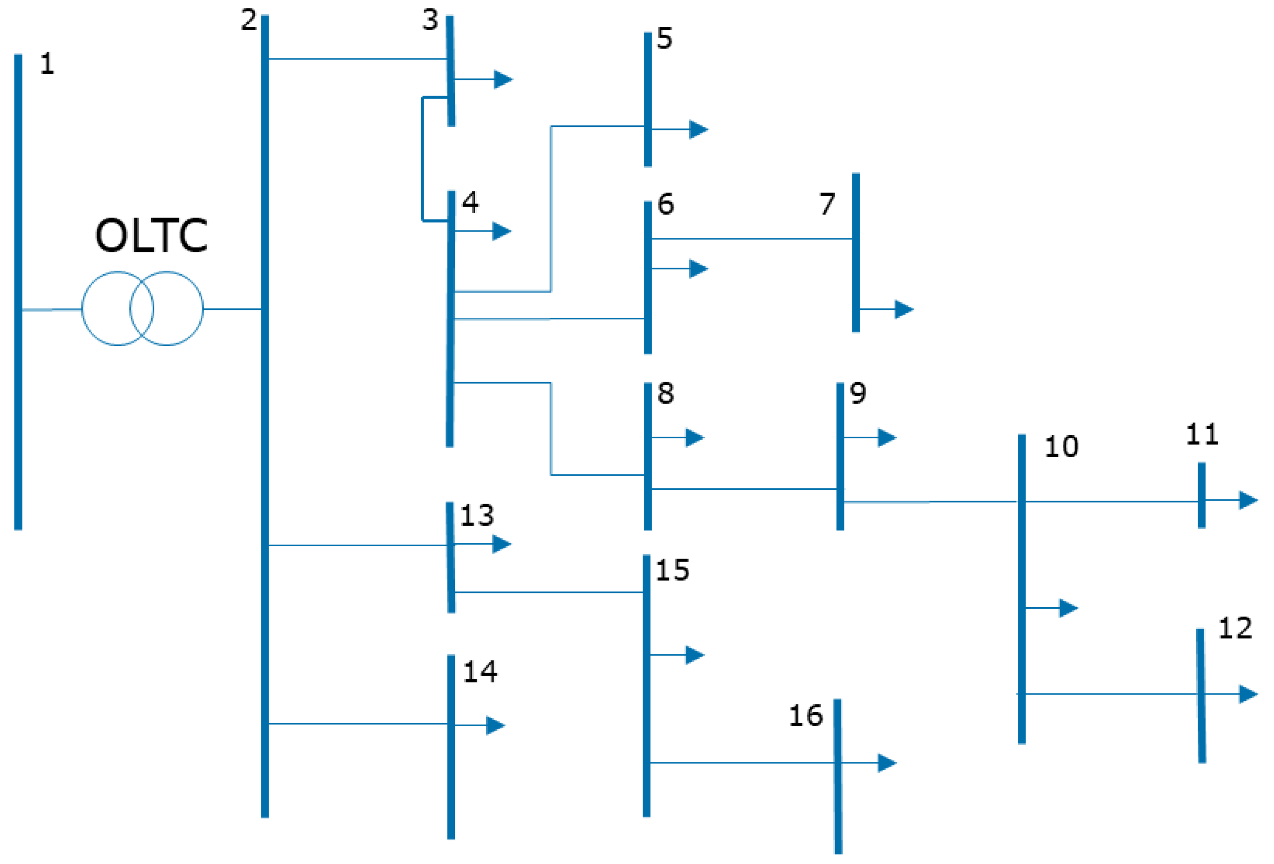
A 16-bus 33 kV radial distribution, as shown in
Figure 1, was used to assess the proposed method. This distribution power system is made of 16 buses and 18 lines. The daily energy demand is 218.83 MWh, the average hourly consumption is 9.12 MWh, and the peak-demand (at hour 16) is 12.52 MW. Since it is an urban feeder, the DGs are located at buses 6, 9 and 11.
The model was implemented in General Algebraic Modelling System (GAMS). The data required for the optimization process were imported and exported using GAMS Data Exchange (GDX) tool. Since the model is defined as a bilevel model, the optimization algorithm provided the optimal solution for every single scenario. Therefore, the consumers who use the proposed method can obtain the optimal investment decision as the best operation-decisions for every possible scenario of the uncertain parameters.
Network parameters and geographical location of the network are available in [
14]. The tariff used in the simulations, energy (£/MWh) and capacity (£/MW-month) prices, are shown in
Table 1. The peak time was 17–20 h, valley periods were 1–4 h and 23–24 h, and base periods were 5–16 h and 21–22 h. The prices represent the behavior of the Mexican electricity market in the daily market [
15] and the capacity market [
16] of Valle de Mexico area. Valle de Mexico is a region in the southern-central part of the Mexican Republic where the capital, Mexico City, is located. Despite this work being developed using the Mexican spot market prices, the market model and its prices are close to any competitive market and, therefore, the results are fairly relevant to any other market.
The price of the energy delivered to the network used in the simulations was , where the discrete probability distribution of the price multiplier μ ranging from 0.9 to 1.1.
The first simulation was carried out considering three different approaches: deterministic model,
EV, and
VaR. The profit obtained by the DG unit,
ProDGe, is calculated as the savings
and revenue
minus the DG expenses (17). It is relevant to note that CAPEX does not change with the price scenario
, since the investment problem is defined in the first-stage.
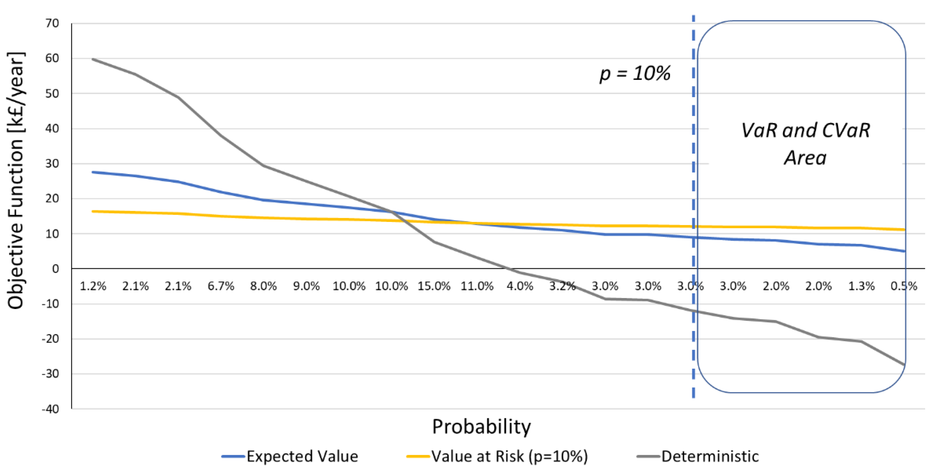
Figure 2 depicts the profit,
ProDGe, obtained by the DG unit. The
x-axis shows the probability while
y-axis indicates the benefits for every scenario. The deterministic curve, which is somehow arbitrary because its results depend on the specific price considered, was calculated using the following two steps: firstly, running the deterministic model for a specific price and finding the optimal DG size and location
; secondly, fixing the DG solution and calculating the objective function
for every realization of the stochastic parameter.
The EV approach maximizes the profit considering all scenarios in the PDF. The p-VaR approach estimates the best value among all worse outcomes whose combined probability is p.
The slope of the curves is the measurement of the uncertainty that the customer can face in the long-run. When the risk is not considered explicitly (deterministic model), the benefit can be 60 k£/year in the best case or −27 k£/year in the worst case. Using the
EV and 10%-
VaR (stochastic approach), the benefit changes dramatically as a consequence of the price uncertainty.
Table 2 presents the values of the maximum/minimum
and the 10%-
VaR and
EV (in k£/year).
VaR is the most conservative approach: no big profits, no relevant losses. Therefore, the chart showing the objective function versus scenarios tends to be flatter. In this test case, the deterministic approach is not only volatile, but also it provides a lowest EV.
Utilizing either
VaR or
CVaR, it is always a challenge to choose the correct value of
. In order to analyze incidence
p,
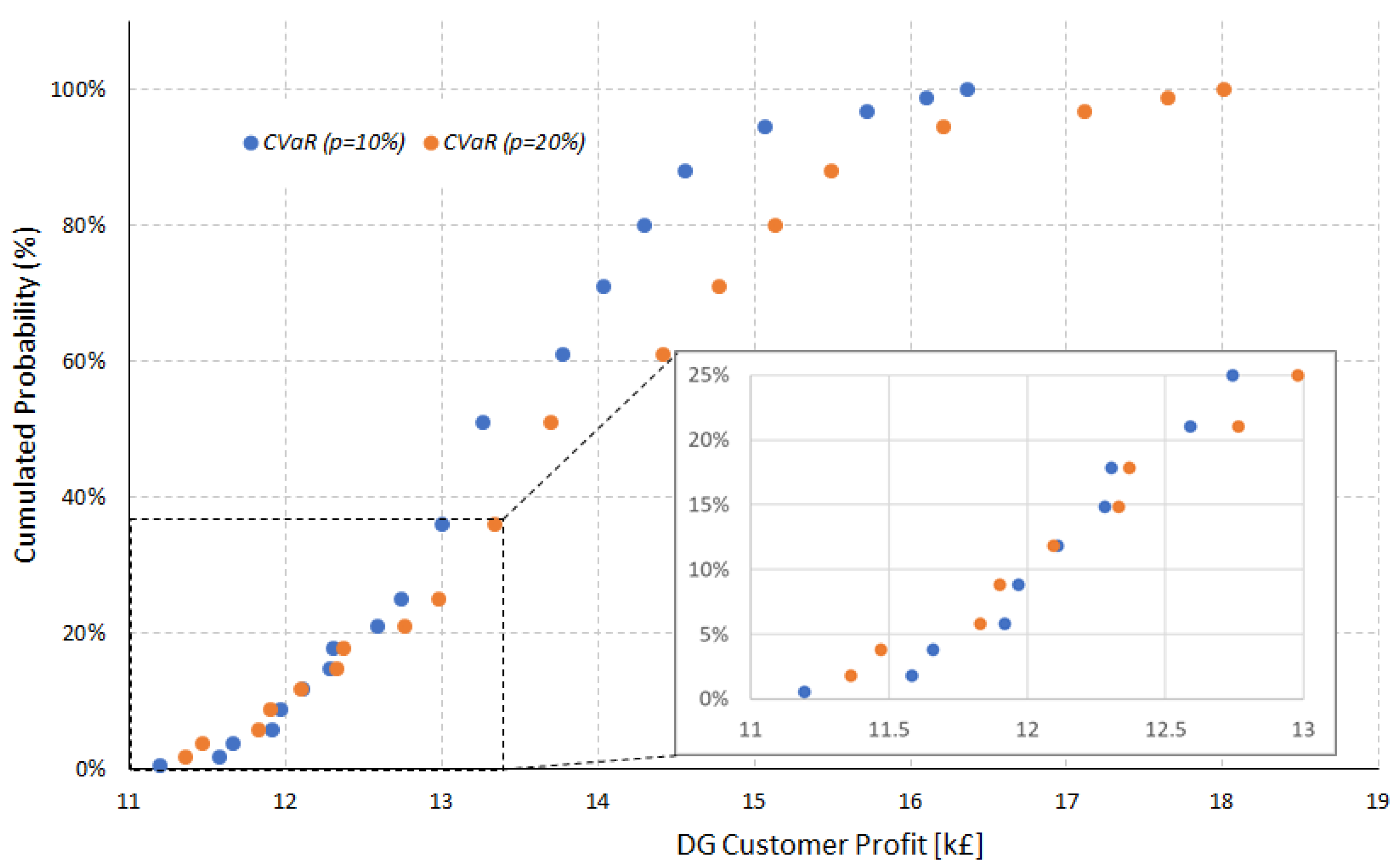
Figure 3 shows the customer benefit using
CVaR with
and
. Risk-averse consumers can choose higher
values since it reduces the risk exposure in the worst-case scenarios. The customer needs to be aware of this conservative approach, which lowers the expected value of the benefit.
Table 3 compares the risk indicators under different risk criteria as objective function.
The Levelized Cost of Energy (LCOE) is the production cost considering the investment and the energy produced (LCOE = Investment Cost/Energy Production). In this particular case, the LCOE was calculated using annual values. Thus, LCOE assumes the following value: .
The decision on the optimal size of DG to be installed depends on the relation between the price of the energy delivered to the network,
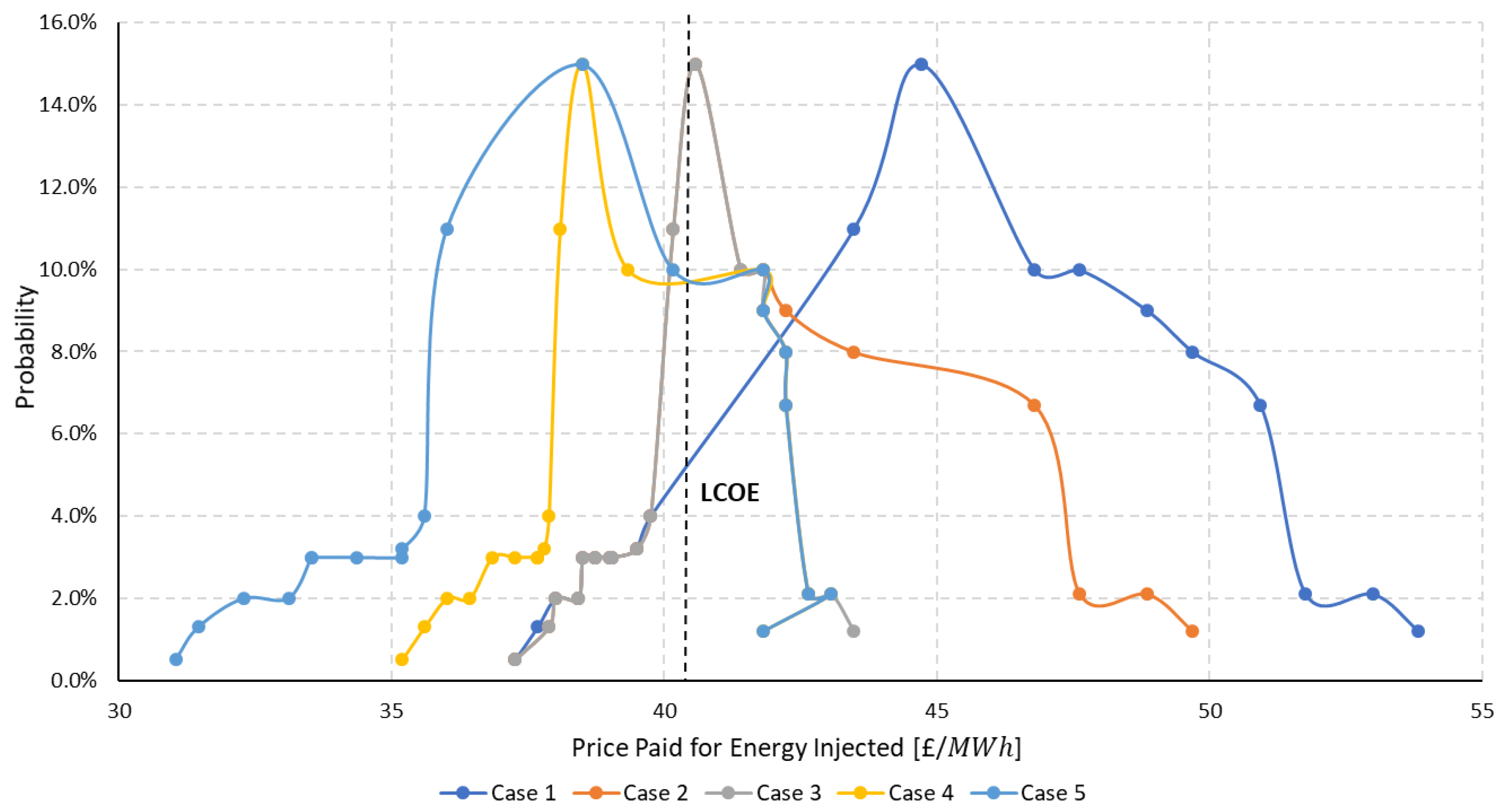
, and LCOE. Then, it will evaluate five cases (see
Table 4) with different PDFs (
Figure 4), with diverse expected values of the price of the energy injected and taking lower and higher values than LCOE.
When the price paid for the energy delivered to the network,
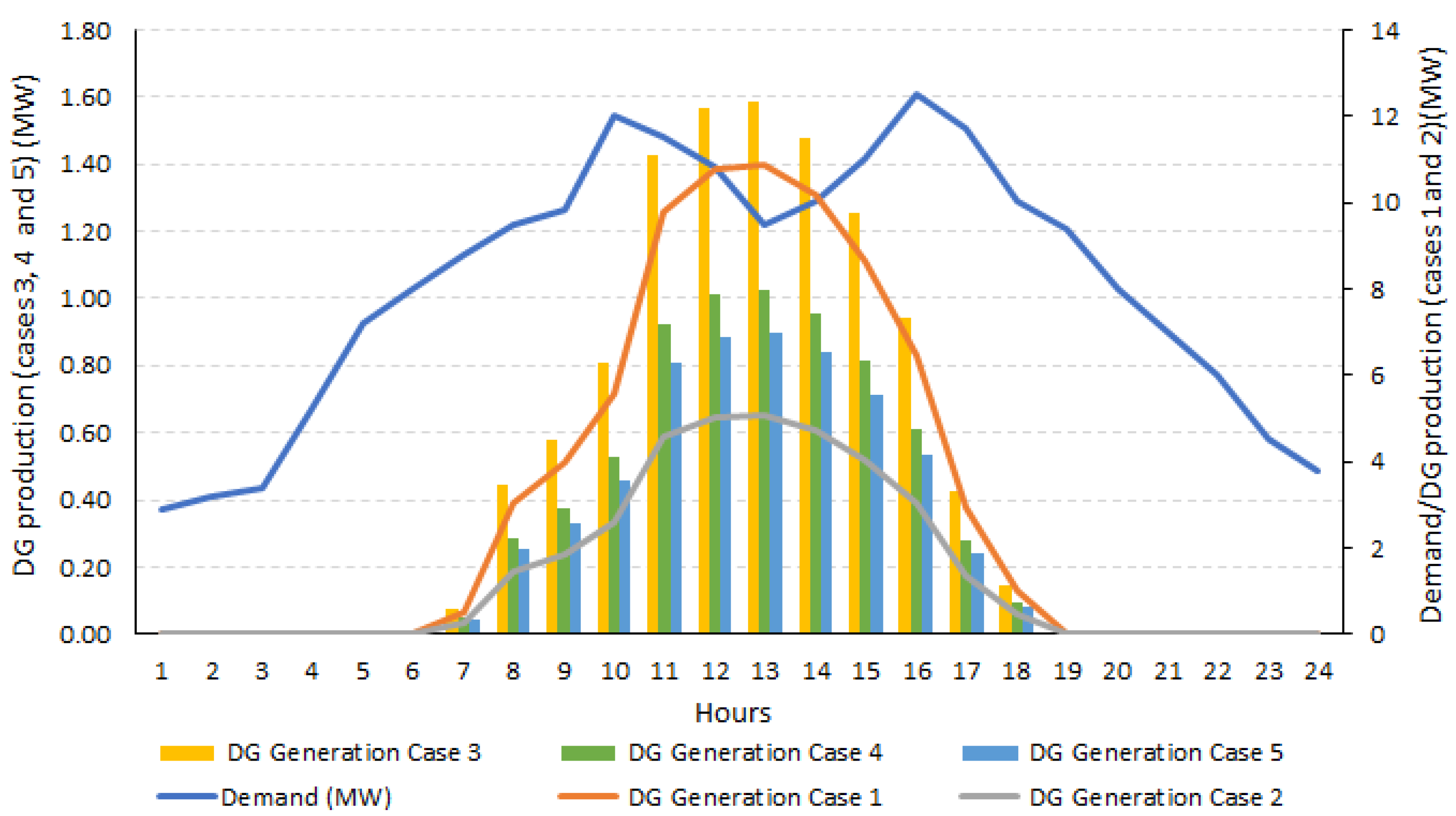
, is higher than LCOE (cases 1, 2 and 3), the energy injection to the network increases as well as the customer profit, as shown in
Figure 5. The higher the price (case 1), the bigger the power injected to the grid.
Otherwise, when the prices are lower than LCOE (cases 4 and 5), the energy injection does not provide benefits for the customer. It is evident from
Figure 5 that the maximum power generation (case 5, hour 13) is about 10 times lower than the highest power generation in case 1. Thus, the optimal amount of DG installed is mostly intended to reduce the customer consumption, because the price of energy consumption remains unchanged.
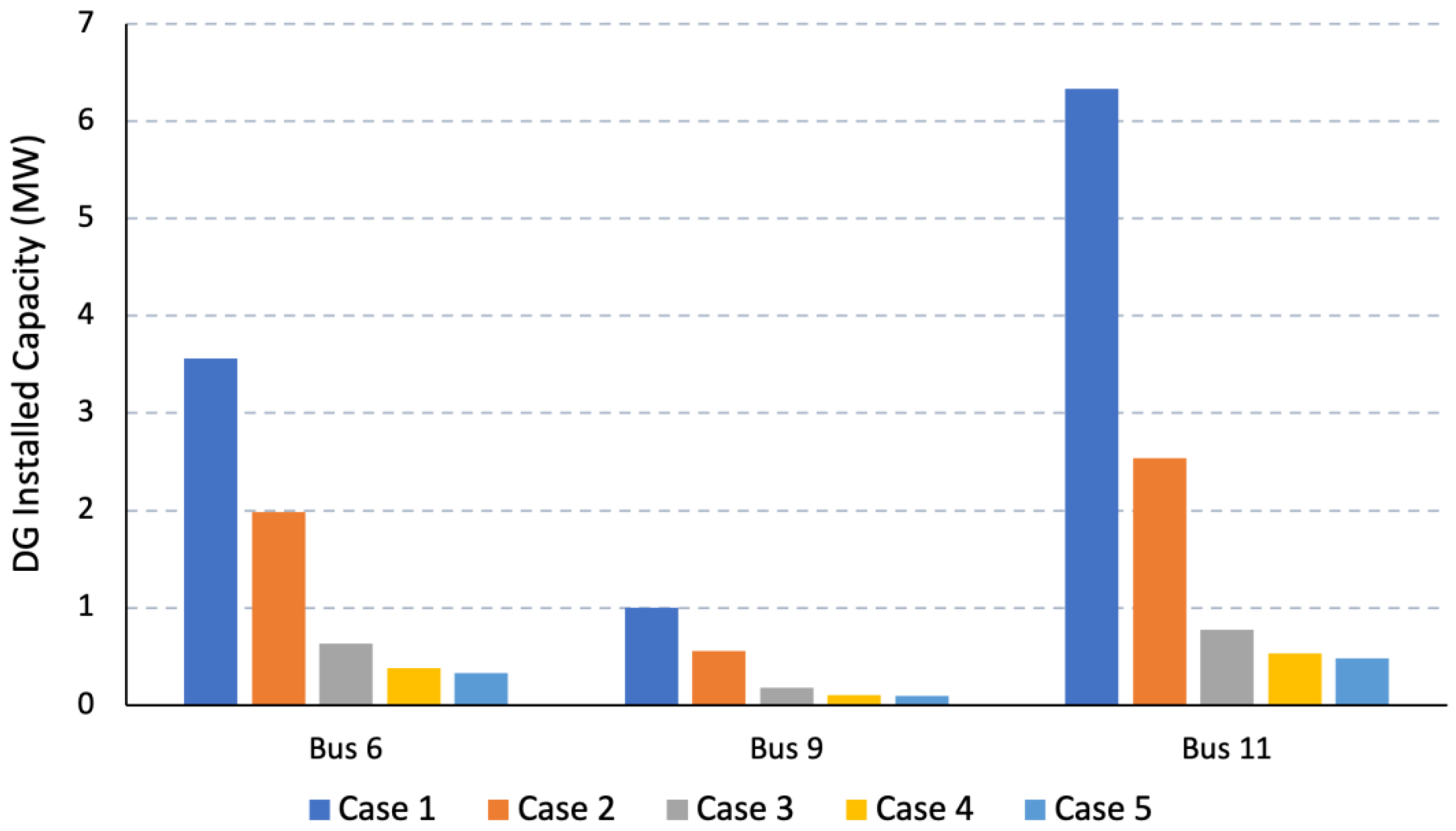
Finally,
Figure 6 shows the size of the DG installed (MW) depending at each bus (6, 9, or 11) and the price paid for the energy injected to the network (Expected Value of each case: 1–5). Obviously, the highest power installed in each bus is obtained in case 1 (high EV). Bus 11 is the best location to install the highest number of DGs.
