1. Introduction
In 2019,
emissions related to the operation of buildings have reached a historical peak of 10
, representing 28% of total global carbon dioxide emissions, as shown in the latest reports of the Global Alliance for Buildings and Construction [
1]. While the energy intensity of the building sector has been steadily decreasing since 2010, an average annual floor area growth rate of around 2.5% has been enough to offset this trend [
2]. This highlights a vast energy efficiency potential, linked with building energy codes lagging behind in emerging economies and renovation rates remaining low in developed nations. In Europe, only about 1% of the existing building stock is renovated each year, but energy retrofitting projects might have the potential to lower the EU’s total
emissions by 5% [
3].
The lack of methods to accurately quantify the savings generated by energy efficiency projects represents a significant barrier towards the attraction of financial investments in this field [
4]. In recent years, investments in renewable energy worldwide have been higher than those in energy efficiency by approximately 20% [
5]. One of the reasons is the possibility of directly metering the energy generated (and therefore the return on investment), as opposed to rough estimations of savings in the case of energy renovation projects. Afroz et al. highlighted how the use of different baseline models can provide very different savings results, and how it is becoming a usual practice in the industry to prefer practical and intuitive models to more sophisticated ones with higher accuracy but poor interpretability [
6]. Additionally, different studies have shown that accurately quantifying the uncertainty of obtained savings estimates is of utmost importance in energy efficiency projects, but that the commonly employed methods have a tendency to underestimate said uncertainty [
7].
Alongside traditional energy efficiency programmes, in recent years, new business schemes are arising from the intersection between energy efficiency and demand side flexibility [
8]. Projects with these characteristics require advanced baseline estimation techniques that are able to accurately and dynamically estimate both energy savings and dynamic uncertainty bands at the hourly or sub-hourly level. Two schemes worth mentioning in this field are Pay for Performance (P4P) [
9] and Pay for Load Shape (P4LS) [
10], in which customers are dynamically compensated for changing their consumption load shape in order to match the evolving conditions of the grid. These new approaches that combine energy efficiency and demand side flexibility arise from a necessity of not only lowering the overall energy usage intensity of the built environment, but also creating a permanent shift of the consumption curve in order to match the hours of highest energy production from renewable sources [
11]. These findings highlight that novel measurement and verification (M&V) methodologies that are able to accurately estimate achieved hourly savings and uncertainty bands, as well as displaced loads, have the potential of unlocking considerable investments in energy efficiency [
12].
1.1. M&V Background
One of the main applications building energy baseline models are used for is the measurement and verification of energy efficiency savings. The International Performance Measurement and Verification Protocol (IPMVP) defines measurement and verification as the practice of using measurements to reliably determine actual savings generated thanks to the implementation of an energy management program within an individual building or facility [
13]. As energy savings are a result of not consuming energy, they cannot be directly quantified. The usual approach for estimating savings achieved by energy efficiency initiatives is to compare the energy usage of the facility before and after the application of the intervention, while also implementing the required adjustments to account for possible changes in conditions. In M&V, there are two main guidelines that are globally recognized: the International Performance Measurement and Verification Protocol (IPMVP), and the ASHRAE Guideline 14 [
14]. Both these protocols are based on the adoption of a baseline energy model to compare the energy performance of the investigated facility before and after the implementation of an energy efficiency measure. The baseline model has the goal of characterizing the starting situation of the facility and it is used to separate the impact of a retrofit program from other factors that might be simultaneously impacting the energy consumption.
1.2. Bayesian Paradigm in M&V
Bayesian methodologies have been proven to hold great potential for M&V, by providing richer and more useful information using intuitive mathematics [
15]. As this article is mainly focused on Bayesian applications in the M&V setting, a full explanation of the theory behind the Bayesian paradigm is out of its scope. Readers are instead referred to the following texts: [
16,
17,
18]. The added value provided by Bayesian inferential methods is linked to their coherent and intuitive approach to the M&V questions, as well as to their probabilistic nature, which enables automatic and accurate uncertainty quantification when estimating energy savings [
19]. Shonder and Im [
20] showed the Bayesian approach to be a coherent and consistent methodology that can be used to estimate savings and savings uncertainty when performing measurement and verification calculations. Lindelöf et al. [
21] tested the Bayesian approach to estimate the savings coming from an ECM implementation, and stressed the clear interpretability and communicability of the results obtained with the Bayesian method. The advantages of communicating to decision makers not only point estimate results, but whole probability distributions with the additional information included. Grillone et al. [
22] gathered together the latest Bayesian specifications for M&V. Among the different reviewed techniques, Gaussian mixture regression [
23] and Gaussian processes [
24] stand out because of their ability to capture nonlinear relationships between variables.
1.3. Multilevel Models
One of the model specifications implemented in this work is multilevel regression. Multilevel (also known by the names of hierarchical, partial pooling, or mixed effects) models are interesting model specifications that prove useful when the analyzed data can be grouped into clusters of similar behavior. More specifically, multilevel models allow the
pooling of information between the different clusters present in the data, meaning that the model learns simultaneously about each cluster while learning about the population of clusters [
16]. In recent years, also thanks to the increase in computing power, multilevel models have attracted great interest and have been applied in many different fields of science and technology [
25]. In the energy field, they have found application in the calibration of building energy models [
26,
27], the forecasting of electricity demand [
28,
29,
30], estimation of overhead lines failure rate [
31], estimation of photovoltaic potential [
32], and the analysis of the degradation of electric vehicle batteries [
33]. In the M&V setting, Booth et al. [
34] used a hierarchical framework to generate energy intensity estimates for various dwelling types. These estimates were then used to calibrate the parameters of an engineering based bottom-up energy model of the housing stock.
1.4. Present Study
Although some research has been carried out on the use of Bayesian methods for M&V, to the best of the authors’ knowledge, no paper has introduced a Bayesian linear regression model, with clear interpretability of the parameters and providing high granularity predictions. Some published works proposed a Bayesian approach with physical interpretability of the coefficients [
21], but only providing predictions with monthly granularity, while others focused on extending the Bayesian approach to high frequency time-series predictions, at the cost of reducing the model interpretability [
23,
24]. Our scope in the present work is to introduce a Bayesian linear regression model that can be easily interpreted and explained to stakeholders, but that at the same time can be applied to time-series with high granularity and can provide accurate and dynamic hour by hour consumption and uncertainty estimates. The model proposed was tested on one of the largest publicly available datasets of non-residential building energy consumption, creating in this way a benchmark for future studies.
The model proposed in this article uses time features and coefficients marking the temperature dependence of the building, while also including information about its typical consumption profile patterns, detected using a clustering algorithm. All the parameters of the model have a clearly interpretable meaning, and the Bayesian approach is able to automatically estimate what the heating and cooling change-point temperatures of the building are, that is, the outdoor temperatures below/above which a significant relationship between the building’s energy consumption and the outdoor temperature conditions is detected. The methodology comes with several advantages:
The model is explainable and its coefficients have a clearly interpretable meaning, a feature which is highly valued by investors in building energy renovation and other stakeholders of the industry.
As the model is probabilistic, uncertainty is estimated in an accurate, automatic, elegant and intuitive way.
The model coefficients and target variables are expressed in terms of probability distributions instead of point estimates, providing a range of additional actionable information to stakeholders.
The provided uncertainty ranges are characterized by dynamic locally adaptive intervals, reflecting how the uncertainty is not symmetrically distributed around the mean of the predictions, and that the values can vary depending on the distribution of the explanatory variables.
The methodology provides extra useful information for stakeholders, such as the typical consumption profile patterns of the building, as well as the probability distributions of the heating and cooling change-point temperatures and of the heating and cooling linear coefficients.
Since Bayesian models are fit to provide reasonable results even when the training data available are scarce, the methodology is well-fit to solve M&V problems, where it is not always feasible to obtain long training time-series with high granularity. Furthermore, the model also has high applicability since the data required is limited to hourly electricity consumption and outdoor temperature values, which are fairly easy to obtain.
The mentioned advantages represent a significant advance to the state-of-the-art, widening the scope of M&V applications and providing the necessary risk mitigation required by financial institutions, thanks to an automatic, dynamic and accurate estimation of uncertainty intervals. Furthermore, the possibility of computing locally adaptive uncertainty ranges can be of fundamental value in those projects where the time-allocation of the savings is as important as the savings themselves. The approach was tested on an open dataset containing electricity meter readings at an hourly frequency for 1578 non-residential buildings. The dataset was collected within the framework of the Building Data Genome Project 2 [
35] and was partly used in the Great Energy Predictor III competition hosted in 2019 by ASHRAE [
36]. Different model specifications were tested on the buildings contained in the dataset, in an attempt to identify their effect on the final accuracy of predictions. This model comparison process was structured in four consecutive phases, which are described in detail in
Section 2.2. The article is structured as follows. First, the methodology is described in detail, together with the model comparison process. Then, the case study is presented and the results obtained are displayed and discussed. Finally, conclusions are drawn and future work recommendations are made.
2. Methodology
In the present article, a Bayesian linear regression methodology capable of providing detailed characterization of building energy consumption, as well as high granularity baseline energy use predictions, is introduced. Different Bayesian model specifications were tested and mapped to changes in the accuracy of hourly energy consumption predictions for a dataset of more than 1500 buildings. Various model variables, prior distributions, and posterior estimation techniques were compared, as well as the effect of implementing a multilevel regression in place of a classical single-level model. The different model specifications were tested on the same dataset, and the results were compared in terms of CV(RMSE) and coverage of the uncertainty intervals. In the following paragraphs, first, the characteristics of the proposed Bayesian approach are presented in detail. Then, the procedure and metrics used to perform the model comparison are discussed.
2.1. Bayesian Methodology
The main aim of the Bayesian inference methodology proposed in this article is to characterize the energy consumption dynamics of individual buildings by means of a linear regression model that uses time and weather features as predictors. The development of such a model enables a deeper understanding of the analyzed buildings’ energy performance and the generation of baseline energy use predictions. In the framework of Bayesian inference, this model is estimated by applying Bayes’ theorem [
17] as follows:
where
M are the model parameters and
D are the measured data.
is the conditional probability of the model parameters’ values, given the measured data from the building; this is also called
posterior distribution.
is the probability of measuring the observed data, conditional on the model parameter values; it can also be called
likelihood.
represents the prior knowledge of the modeler about the plausible distribution of the model parameters; this is referred to as the
prior probability distribution.
represents the probability of observing the data and is usually called
marginal probability or
marginal likelihood. In practical terms, we define a regression model, aimed at estimating building energy consumption values based on time and weather features, then we provide to this model a set of measurement data, a prior probability distribution of the model parameters (based on our previous knowledge of building physics) and a likelihood function for the observed data. Through the formula in (
1), the Bayesian inference model is then able to provide a posterior probability distribution of the model parameters and of the target variable (electricity consumption). The model and target variable posteriors can then be used to characterize the energy consumption of the analyzed building and to generate baseline energy consumption predictions and uncertainty bands. The flowchart in
Figure 1 represents the structure of the proposed methodology, including the initial phase of data pre-processing in which a clustering algorithm is used in order to detect recurrent daily load profiles in the building, which then are used as data for the regression model. In the following, the technical details of the presented methodology are presented and discussed.
2.1.1. Data Pre-Processing
The first step of the proposed Bayesian approach is a data pre-processing phase that is critical in order to build the dataset that is used in the analysis. The pre-processing workflow consists of the detection of clusters of days that have similar electricity usage patterns. In order to implement the pattern recognition algorithm, the data are first transformed through the following steps:
The original frequency of the consumption data is resampled (aggregated) to have one value per 3 h (8 values per day);
For each day in the time-series, the consumption values are transformed into daily relative values . ;
A matrix of relative consumption values is generated, having as rows the days of the time-series and as columns the 8 parts of the day defined in point 1;
The values in the matrix are transformed with a normalization between 0 and 1. This enables more accurate predictions with the clustering algorithm.
To detect the profile patterns, a spectral clustering methodology is implemented [
37]. This specific clustering technique is performed by embedding the data into the subspace of the eigenvectors of an affinity matrix. This is done through the use of a kernel function, specifically, the one used in this application was a radial basis kernel, also known as a Gaussian kernel. Using this kernel, an affinity matrix
that is positive, symmetric and depends on the Euclidean distance between the data points is defined:
Then we define the degree matrix
, a diagonal matrix that summarizes the affinity of each element of
A with all the other elements of the matrix. Using the affinity and the degree matrices we can calculate the unnormalized graph Laplacian:
If the analyzed data are actually spaced so that there are different clusters, the Laplacian L will then be approximately block-diagonal, and each block will define a cluster. From the analysis of the eigenvalues and eigenvectors of L, it is possible to estimate what the optimal number of clusters is.
Once the recurrent daily profiles have been detected for the training year, a classification algorithm calculates the cross Euclidean distance matrix between the detected cluster centroids and the load curve of each day of the test year, assigning them to one of the identified clusters.
2.1.2. Regression Model
The linear regression model developed in this work is based on several coefficients aimed at capturing the dynamics that drive the energy consumption of the analyzed buildings. The hourly energy consumption of the building is supposed to be partially dependent on time-features such as the hour of the day, and partially on thermal dynamics driven by outdoor temperature variations. In the estimation of the temperature-dependent term, a heating change-point temperature and a cooling change-point temperature are defined—the outdoor temperatures below/above which a significant relationship between the building’s energy consumption and the outdoor temperature conditions is detected. This model structure is based on the concept of linear change-point models, first introduced in the literature with the PRISM method [
38]. The coefficients of the model, with the exception of the change-point temperatures, are supposed to vary depending on the load profile of the day (detected with the clustering algorithm previously introduced), or on the day-part, a fictitious variable generated after dividing the day in 6 day parts of 4 hours each. The mathematical description of the Bayesian linear regression model used follows, where the square brackets notation has been used to represent the variables that have a different value for each profile cluster
k or day-part
j. The
likelihood assigned to the observed variable (hourly electricity consumption) was a normal distribution with mean
and standard deviation
:
where:
is the intercept of the model, one for each profile cluster k detected,
represents the effect of the hour of the day , following a Fourier decomposition with n harmonics. and are the linear coefficients that mark the weight of each hour on the final electricity consumption; one for each profile cluster k detected and for each harmonic p.
and are the coefficients that represent the piece-wise linear temperature dependence of the model, one for each day-part j previously defined.
and are the difference between the outdoor temperature and the change-point temperatures detected by the model for heating and cooling.
and are logical variables making sure that the temperature-dependent term is only evaluated when the outdoor temperature is above/below the cooling/heating change-point temperature:
and are two logical coefficients that are automatically optimized by the model and that mark whether or not a certain profile cluster k has heating or cooling dependence.
The predictors used in the regression model were one of the model specifications that were evaluated in the model comparison stage. More specifically, the inclusion of a wind speed predictor was also tested when comparing different model specifications. The mathematical formulation of the second model tested in the comparison stage (with the addition of the wind speed term) follows:
where linear dependence between the energy consumption and the wind speed
were supposed, with coefficient
, depending on the day-part
j. Finally, it is important to note that, for both regression models, a log-transformation of the target variable was performed, in order to improve the prediction accuracy.
2.1.3. Prior Probability Distributions
An important step of Bayesian modeling is to choose the prior probability distributions of the model parameters. These values express the belief the modeler has about the probability distribution of the parameters before analysing the data. If no previous information is known about the probability distribution of the parameters, then a uniform prior with a lower and an upper bound is a common choice, meaning that all the values contained between the two boundaries have the same prior probability. In order to test the effect of more or less informative priors on the accuracy of the model predictions, the model was first run with uniform priors on most of the parameters. The uninformative priors set were the uniform distributions with different lower and upper bounds:
In the model comparison stage, a set of regularizing prior distributions was also implemented, in order to test their impact on the accuracy of the model predictions. A presentation and discussion of the regularizing priors used the following:
For the model intercept and the time features coefficients and , a weakly regularizing normal prior distribution, centered in 0 and with a standard deviation equal to 1 was set. For the heating and cooling coefficients and , a half-normal prior with a standard deviation equal to 1 was used. This prior distribution assigns zero probability to negative values of the temperature coefficients, according to the intuition that outdoor temperature deviations above the cooling change-point temperature, or below the heating change-point temperature, will result in the electricity consumption of the building either increasing () or staying unchanged (). For the change-point temperatures, a uniform prior was used, ranging between the minimum and the maximum outdoor temperatures observed in the training data and . The priors of the dependence coefficients and were modeled as a Bernoulli distribution with probability , giving them an equal prior probability of being either 0 or 1.
2.1.4. Pooling Techniques
Previously, a description was provided of how, in the pre-processing phase, the days of the time-series are clustered according to the shape of the load curves. In the construction of a model for observations, which are grouped together on a higher level, there are two conventional alternatives: either modeling all the observations together independently of the clusters they belong to, or calculating independent coefficients for each of the clusters. The advantages and disadvantages of these two approaches have been widely analyzed in the framework of the bias–variance trade-off discussion [
39]. In this article, we decided to explore a third option as well, which is referred to here as
partial pooling, and that also goes by the name of multilevel, hierarchical, or mixed effects regression. The term partial pooling refers to the action of
pooling information between different clusters during the modeling phase. In our case, a
complete pooling approach would be equivalent to the first of the previously mentioned alternatives—to assume that there is no variation between days having different load shapes, and to produce a single model estimate for the model parameters, independently of the clusters. The
no pooling approach, on the other hand, would be to assume that the variation between the clusters is infinite, therefore nothing learned for days with a certain load shape can help predict days belonging to a different cluster. The partial pooling approach produces estimates by including in the model individual coefficients for each of the detected clusters (similar to the no pooling case) but with the additional assumption that these same coefficients have a common prior distribution that is adaptively learned by the model [
16]. In other words, in multilevel regression, although individual model parameters are estimated for each cluster, the information provided by each cluster can be used to improve the estimates for all the other clusters.
When translating this into a mathematical formulation, the only difference from a traditional Bayesian regression model without multilevel structure is that, instead of the usual prior distributions, an adaptive prior is defined. The adaptive prior is a function of two additional parameters, often referred to as hyperparameters, and that in turn have a prior distribution, called a hyperprior. In the context of this article, we decided to test whether pooling information among different clusters when estimating the intercept and time features coefficients could improve the model performance. The following adaptive priors were tested in the model comparison stage, in place of the regularizing priors defined in the previous section:
The advantage of multilevel regression is that it is still possible to include in the model the variability caused by the higher level variables (load shape clusters in this case) but, at the same time, overfitting is avoided by stating that the priors of the model coefficients related to those variables are drawn from a common distribution. The partial pooling estimates will be less underfit than the average coefficient from the complete pooling approach, and less overfit than the no-pooling estimates. This turns out to be particularly strong when there is not so much data available for some of the categories, because then the no pooling estimates for those clusters will be especially overfit [
16]. On the the other hand, when there are plenty of data for each of the groups, the effect of implementing multi-level regression turns out to be less influential on the final result; this is why we decided to test whether or not implementing this technique might have a positive effect on the accuracy of the model predictions.
2.1.5. Posterior Estimation Methods
According to the theory of Bayesian statistics, after defining the required variables, Bayesian models update the prior distributions previously set to obtain the posterior distribution. A unique posterior distribution exists for each combination of data, likelihood, parameters, and prior. This distribution represents the relative plausibility of the possible parameter values, conditional on the data and the model. Historically, being able to effectively estimate the posterior has always been one of the main practical issues of Bayesian modeling. Starting from the 1990s, thanks to the access to cheap computational power, Markov chain Monte Carlo (MCMC) [
40] methods started being the prevailing technique used for posterior estimation purposes in Bayesian modeling. MCMC approaches follow the idea that, instead of computing a direct approximation of the posterior, which is many times unfeasible from a computational point of view, such an approximation can be obtained by drawing samples from the posterior. The samples drawn provide a set of possible parameter values, and their frequency represents the posterior plausibilities. One of the most popular MCMC algorithms used in practical applications is the Hamiltonian Monte Carlo (HMC). Originally proposed in 1987 by Duane et al., this algorithm is able to draw samples more efficiently by reducing the correlation between them thanks to the simulation of Hamiltonian dynamics evolution [
41]. In the present research, HMC is one of the techniques used for posterior estimation. More specifically, the No-U-Turn Sampler (NUTS) algorithm was used: an extension of the HMC algorithm that provides accurate and efficient posterior samples without needing user intervention or tuning runs [
42].
One of the drawbacks of MCMC methods is that when models start having a very high number of variables and data points, their computational cost becomes extremely high. Automatic Differentiation Variational Inference (ADVI) is an alternative technique that resolves the problem of the computational bottleneck by turning the task of computing the posterior into an optimization problem [
43]. First, for a given set of model parameters
and observations
x, a family of distributions
, parametrized by a vector
is hypothesized. The optimization is then aimed at finding the member of that family that minimizes the Kullback-Leibler (KL) divergence to the exact posterior:
Since the KL formulation involves the posterior, and therefore does not have an analytic form, rather than minimizing the KL, the analysis is aimed at maximizing the evidence lower bound (ELBO):
is equivalent to the opposite of the KL divergence, up to the constant
, hence maximizing the ELBO is equal to minimizing the KL divergence [
44].
When comparing MCMC methods to ADVI, the first are often more computationally intensive, but they have the advantage of providing (asymptotically) exact samples from the posterior. Variational inference, on the other hand, is aimed at estimating a density that is only close to the target and tends to be faster than MCMC. This makes ADVI the best choice when the objective of the analysis is testing many different models on large datasets. MCMC is often used with smaller datasets, when computational time is not an issue, or in specific situations where the higher computational cost is not considered a problem compared to the added value of obtaining more precise posterior estimations [
45].
In this article, the computational cost of MCMC methods was recognized as a possible issue, therefore ADVI was used as the main posterior estimation technique. Only in the last phase of model comparison, considering the fact that ADVI is an optimization algorithm that does not guarantee to provide exact samples from the target density, the posterior was estimated with both ADVI and MCMC sampling techniques. This allowed us to evaluate whether or not the ADVI approximation was producing models that performed significantly worse for our use-case.
2.1.6. Uncertainty Intervals
One important difference between Bayesian statistics and traditional frequentist methods is related to how they quantify uncertainty. More specifically, when defining uncertainty intervals for model predictions, Bayesian methods give rise to
credible intervals while frequentist methods generate
confidence intervals. Although having similar names, the meaning and interpretation of these statistical concepts are profoundly different. This is connected to the inference problems that these two approaches to statistics are seeking to answer. The Bayesian inference problem is the following: given a set of model parameters
and observed data
D, what values of
are reasonable given the observed data? On the other hand, the inference question asked by the frequentist approach is: are the observed data
D reasonable, given the hypothesised model parameter
? This results into two different approaches to the modelling process: while frequentists consider
to be fixed and
D to be random, Bayesians consider
to be random and
D to be fixed [
46]. This gives rise to the different interpretation the credible and confidence intervals have: computing a 95 % credible interval is equivalent to stating “given the observed data
D, there is 95% probability that the model parameter
will fall within the credible interval”. On the other hand, since in the frequentist approach, the parameters are fixed, while the data are random, computing a 95% confidence interval means stating “if the data-generating process that produced
D is repeated many times, the computed confidence interval will include the true parameter
95% of the times”. Therefore, while the Bayesian solution represents a probability statement about the parameter values, given fixed interval bounds, the frequentist solution concerns the probability of the bounds, given a fixed parameter value. Credible intervals capture the uncertainty in the parameter values and can therefore be interpreted as probabilistic statements about the parameter. Conversely, confidence intervals capture the uncertainty about the computed interval (i.e., whether the interval contains the true value or not). Thus, it is not possible to interpret confidence intervals as probabilistic statements about the true parameter values. The frequentist method is not wrong, it is just answering a different question, that usually tells us nothing about the specific dataset we have observed. In fact, when dealing with one specific dataset (which is usually the case in the M&V setting), all that a confidence interval can say is: “for this specific dataset, the true parameter values are either contained or not contained in the confidence interval”.
In order to better clarify these concepts, a practical example of the energy baseline modelling case will be presented. We suppose that two energy baseline models have been estimated—one Bayesian and one frequentist—with the corresponding uncertainty intervals. In the Bayesian case we are able to state the following: given the training data observed (energy consumption and outdoor temperature time-series), there is 95% probability that the estimated model parameters (and therefore the predictions) will fall within the calculated credible interval. On the other hand, the corresponding frequentist statement would be: if we could repeat many times the data-generating process that leads to the energy consumption and outdoor temperature values that we observed, 95% of times the estimated model parameters would be included in the calculated confidence interval. It is evident that, for the case in analysis, the Bayesian interpretation is the one which is the most reasonable and coherent. Despite this, it is fair to state that, for many common problems, such as linear regression, the Bayesian and frequentist intervals can coincide. This is also the reason why, in many contemporary scientific studies, Bayesian interpretation is (erroneously) applied to frequentist confidence intervals. Unfortunately, this match ceases many times when the models start becoming more complex than standard linear regression [
47]. An additional feature of Bayesian credible intervals is that, while confidence intervals are delimited by two (random) numbers, credible intervals are represented by probability density functions, which are visibly more suited to risk assessment or uncertainty quantification problems [
15].
In many Bayesian studies, including this article, credible intervals are represented as highest posterior density intervals (HDI or HPDI), defined as the narrowest interval containing the specified probability mass. This means that a 95% HDI will be represented by the narrowest interval containing 95% of the probability mass. Frequentist confidence intervals are equal-tailed, since they are generally computed by adding or subtracting a fixed number from the mean. While this can work for symmetrical distributions, real data are often asymmetrical and frequentist equal-tailed intervals will lead to, including unlikely values on one side, while excluding more likely values on the opposite side. HDIs solve this problem by providing local adaptive uncertainty bands with equally likely (but not symmetrical) lower and upper bounds [
19].
2.2. Model Comparison
In this section, the structure of the model comparison that was performed is discussed. The comparison was carried out in four consecutive test phases, which are summarized in
Table 1. The specifications that are tested in each phase are highlighted in the table. The first model run was the benchmark model, to which the others were compared. In the second phase, the goal was to test the use of regularizing priors, while in the third phase the inclusion of a wind speed feature in the regression model was assessed. Finally, in the fourth phase, two different techniques for the posterior estimation were tested, and a comparison was performed between regular regression and multilevel regression. In each consecutive phase, the best performing specification previously tested was then implemented.
2.2.1. Model Comparison Phases
Phase 1
The first test was run using the benchmark regression model with time and temperature features and uniform priors. The coefficients were supposed to have different values according to the detected load profile cluster, but no pooling was performed between the different clusters. The posterior distributions were estimated using the ADVI technique. This is the benchmark model specification to which the following versions were compared.
Phase 2
In the second test, the same regression model of Phase 1 was used, but this time with regularizing priors in place of the flat priors previously used. Again no pooling was performed, and the posterior distributions were estimated using ADVI. This phase was aimed at understanding whether the use regularizing priors, selected using domain knowledge about building energy consumption modeling, could improve the prediction accuracy.
Phase 3
In the third set of model tests, a wind speed predictor was added to the linear regression model, as described in
Section 2.1.2. Regarding the prior choice, it was decided to use whichever priors were granting higher accuracy between the ones tested in Phase 1 and 2. The pooling and posterior estimation techniques used were the same used in the previous phases. This model comparison phase was aimed at understanding whether adding a wind speed feature could improve the prediction accuracy.
Phase 4
In the last model comparison phase, the regression model providing the best accuracy between the one including and excluding the wind speed predictor was used. The best performing priors, already used in Phase 3, were selected again. Different pooling techniques were then compared (partial pooling, no pooling, complete pooling), as well as two different methods to estimate the posterior distributions—ADVI and a HMC sampling through the NUTS algorithm. This phase had the goal of testing whether implementing multilevel regression in place of regular regression could bring added value in terms of model accuracy or uncertainty bands estimation for our use case. At the same time, it was possible to evaluate the goodness of the ADVI posterior approximation by comparing it to the one obtained with the sampling approach.
2.2.2. Comparison Metrics
Three main metrics were used in order to compare the different models tested. The CV(RMSE) was used to assess the prediction accuracy of the model, while the coverage and adjusted coverage parameters were analyzed to evaluate the uncertainty bands estimated.
CV(RMSE)
The coefficient of variation of the root mean square error (CV(RMSE)) is a metric frequently employed to evaluate the accuracy of energy baseline models:
with
N being the total number of hours of the time-series,
the measured energy consumption value at hour
i,
the energy consumption predicted using the regression model, at the same hour, and
the average hourly energy consumption across the whole time-series. Equation (
22) shows how the CV(RMSE) is nothing but a normalization of the root mean square error by the mean of the measured energy consumption values
, representing a comparison between the model error and the average energy consumption values for the selected building or facility.
Coverage
In order to compare the accuracy of the uncertainty intervals estimated with the tested model specifications, the concept of coverage probability was used. When evaluating uncertainty intervals, the coverage probability represents the proportion of times that the real observed value is contained within the estimated interval.
where:
with
N being the total number of hours of the time-series,
the measured energy consumption value on hour
i,
and
the higher and lower bounds of the predicted uncertainty bands for hour
i. One problem of this metric is that, in its evaluation, it does no take into account the size of the estimated uncertainty intervals. A disproportionately large interval would always have 100% coverage, but this can be an indication that the model that generated such interval is misspecified. In order to solve this issue a new metric, called adjusted coverage, was defined. This newly defined metric modifies the traditional coverage concept with additional terms that have the objective of penalizing larger intervals.
where:
This additional metric enables a more accurate comparison of the different Bayesian inference models tested. The traditional coverage concept, which simply checks whether the real value lies within the predicted uncertainty interval, does not provide enough information to correctly compare the bands. The adjusted coverage solves the issues of the coverage metric by adding two penalization terms. The first of these terms is included in , a variable representing whether or not the metered value is contained in the interval. If is within the interval, then is equal to 1, otherwise it is equal to 1 plus a term that is proportional to the distance between the closest bound and the metered value. In this way ’bigger errors’ of the model are penalized more. The second penalization term is , which is proportional to the size of the predicted uncertainty interval. Both terms are expressed as a ratio of logarithms, in order to prevent the adjusted coverage from reaching very high values when the metered or the are close to zero. This metric, although not suitable for a comparison between different buildings, serves the purpose of comparing uncertainty intervals predicted by different models for the same building well. Among models with equal coverage, those having smaller adjusted coverage are to be preferred, since this represents a lower overall model uncertainty.
3. Case Study
The presented approach was tested on an open dataset containing electricity meter readings at an hourly frequency for 1578 non-residential buildings. It was decided to test the approach on this dataset because of the generally recognized need, in the building performance research community, of testing novel techniques on common datasets [
48]. This helps providing meaningful comparisons of accuracy, applicability, and added value between methodologies. The dataset is part of the Building Data Genome Project 2, a wider set that contains readings from 3053 energy (electricity, heating and cooling water, steam, and irrigation) meters from 1636 buildings. Of the original 1636 buildings, only the 1578 containing electricity meter readings were selected, since the proposed methodology has the goal of modeling hourly electricity consumption. A thorough description and exploratory data analysis of this dataset is available in Miller et al. [
35]. A summary of the remarks that might be of interest follows:
the buildings belong to 19 different sites across North America and Europe, with energy meter readings spanning two full years (2016 and 2017);
there are five main primary use categories: education, office, entertainment/public assembly, lodging/residential, and public services;
the weather data provided includes information about cloud coverage, outdoor air temperature, dew temperature, precipitation depth in 1 and 6 hours, pressure, wind speed and direction;
for most of the buildings, additional metadata such as total floor area and year of construction are available.
Table 2 contains an overview of the sites present in the dataset and the number of buildings having electricity meter readings. Each site is assigned an animal-like site code name and each building is characterized by a
Unique Site Identifier consisting of the site code name, an abbreviation of the building primary space usage, and a human-like name unique for each building. An example of a building’s unique site identifier is:
Rat_health_Gaye.
In this case study, the year of 2016 was used to train the model. Validation of the model prediction accuracy was then performed on data from 2017. The CV(RMSE), coverage and adjusted coverage were calculated between 2017 model predictions and observed meter readings.
4. Results
The Results section is divided into two parts. First, the model comparison results are analyzed and the model specifications that produced the highest prediction accuracy are pointed out. Then, the results obtained for two individual buildings are presented in detail, highlighting the outputs of the methodology, such as the clustering of the daily profiles, the change-point temperatures and coefficients detected, as well as predictions for the full test year. All the coverage and adjusted coverage estimations provided in this section are referred to 95% HDIs. Regarding the software used for the analysis, the consumption profile clustering was performed with the kernlab library [
49] in the R programming environment, while the Bayesian models were calculated using the python library PyMC3 [
50].
4.1. Model Comparison
The results obtained for each of the model comparison phases are presented here in form of boxplots for the CV(RMSE), coverage and adjusted coverage variables. It is important to note that the dataset that was selected for the case study contains various buildings for which the test year data are very different from the training year data. Examples of this are buildings with flat consumption in the whole test year or in large parts of it, as well as buildings having completely different energy consumption trends in the training and test year, meaning that no baseline model could provide accurate predictions. In
Figure 2, the electricity consumption time-series of one of these ‘outlier’ buildings is shown. In order to not manually exclude any building from the analysis, while the results for all the buildings were calculated, in the boxplots the outlying values were hidden, meaning values 1.5 IQR above the upper quartile or below the lower quartile are not shown. The analysis performed in this section is based on median values and boxplot analyses that are not affected in any way by the exclusion of the outlier buildings from the plots.
Figure 3 and
Figure 4 show the results in terms of CV(RMSE) and coverage for the first three phases of model comparison. In the second phase of the analysis, the benchmark model of Phase 1 was updated with regularizing priors in place of the uninformative ones previously used. In the third phase, the model from Phase 2, which proved to be better than the benchmark model both in terms of CV(RMSE) and adjusted coverage, was complemented with an additional term marking the effect of wind speed. From
Figure 3 and
Figure 4, we can see that while the use of regularizing priors caused only a slight decrease of CV(RMSE), the uncertainty bands were highly affected by this change. A quick analysis of
Figure 4 shows that, while the model with uninformative priors had the highest coverage, this was mainly due to the estimation of disproportionately large uncertainty bands. The addition of the wind speed term, on the other hand, seems to have no effect on neither the CV(RMSE) nor the coverage of the model, meaning that for this dataset using wind speed as a predictor variable for electricity consumption does not provide any benefit.
The first three phases of the model comparison helped to prove that the regression model and prior distributions used in Phase 2 were the ones providing the highest accuracy with the smallest number of predictor variables. Phase 4, on the other hand, was aimed at testing the performance of multilevel regression and different posterior estimation techniques. In Phase 4, the model of Phase 2, originally characterized by the use of a
no pooling approach and ADVI estimation, was compared with specifications that used the same regression model and prior distributions of Phase 2, but implementing complete and partial pooling as well. The use of the NUTS (MCMC sampling) algorithm for the estimation of the posterior distribution was also tested, using 2000 tuning steps and then sampling four chains with 5000 samples each.
Figure 5,
Figure 6 and
Figure 7 show the boxplots obtained for the final phase of model comparison, while
Figure 8 allows to simultaneously analyze the CV(RMSE) and adjusted coverage metrics. The first clear conclusion that can be drawn is that complete pooling is the least performing of the three pooling approaches, which is coherent with the method used to build the regression model (giving high value to the clustering approach to detect different consumption trends). At the same time, the results obtained show that the use of partial pooling marks a definite coverage improvement over no pooling for the NUTS estimation case, while when using ADVI the two models are practically equivalent. When comparing the posterior estimation techniques, the use of MCMC sampling yields comparable CV(RMSE) and slightly better adjusted coverage over the variational inference approach:
Figure 8 provides a helpful visualisation in this regard.
Regarding the computational time difference between ADVI and NUTS, the analysis was run on a remote server with 125 GB of RAM and an Intel Xeon Processor with 2.60 GHz base frequency, using 12 of the 32 available cores. The average computational times required for the analysis are summarized in
Table 3, which also presents the median CV(RMSE), coverage, and adjusted coverage obtained with each model of Phase 4. It appears that NUTS estimations require around 35 times more computational power than the ADVI case, while providing only modest improvements in terms of adjusted coverage. It is worth mentioning that, for the no pooling and partial pooling cases, the computational time required to model one building is directly proportional to the number of different load profile patterns detected by the clustering algorithm, since each additional load profile increases the number of variables that need to be estimated in the model.
4.2. Individual Buildings
In this section, the model results obtained for two individual buildings are analyzed, in terms of consumption predictions, weather dependence and posterior distributions identified for the model parameters. The results shown are the ones obtained using partial pooling and ADVI posterior estimation.
The first building analyzed is
Rat_health_Gaye, a healthcare facility located in Washington DC with a total floor area of 2220 square meters. The five recurrent load profiles identified by the clustering algorithm for this building are represented in
Figure 9, with the red lines representing the profile centroids and the black lines the load profiles of days belonging to that cluster. In
Figure 10, the electricity consumption time-series for both the training and test years (2016 and 2017) is shown.
At first glance, it appears that this building is using electricity for the cooling system, while a different energy source is used for heating, since the consumption is quite constant during the winter months and peaks in the summer period. An analysis of the change-point temperatures estimated by the Bayesian regression model can help confirm this hypothesis.
Figure 11 shows the posterior distributions estimated for the heating and cooling change-point temperatures, both the mean value and the 94% HDIs are marked.
In order to better understand these results, it can be useful to visualize the electricity consumption and outdoor temperature time-series, together with the heating and cooling change-point temperatures estimated by the model.
Figure 12 shows this relationship for the training year, with the estimated mean heating and cooling change-point temperatures marked as a dotted line, and their 94% HDIs represented by the shaded area. This plot confirms the initial hypothesis and validates the results of the model. The building has cooling dependence: it can be seen how the electricity consumption starts increasing once the outdoor temperatures exceed the estimated cooling change-point temperature. At the same time, the model detected no heating dependence, showing that the heating change-point temperature would correspond to the lowest temperature observed in the training year. This conclusion is confirmed by studying how the electricity consumption does not react to changes in temperature below
.
In
Figure 13 the electricity consumption time-series of the test year is shown (in black), together with the model predictions and 95% uncertainty bands (in red). In order to better visualize the uncertainty bands and predictions,
Figure 14 shows a segment of this same plot that includes only predictions for the month of July 2017, where the building energy consumption is being affected by the outdoor temperature values. Overall, the model is able to accurately predict the consumption time-series of the test year and to capture the temperature dependence dynamics of the building. This model was characterized by a CV(RMSE) of 15.2%, a coverage of 96.7% (for the 95% HDI) and an adjusted coverage of 1.94.
The second case presented is that of a building that has both heating and cooling consumption dependence. The building analyzed is
Rat_education_Royal, a school in Washington DC with a total floor area of 7218.6 square meters. The building electricity consumption time-series for the training and test year is shown in
Figure 15 where it is possible to observe that the consumption is peaking both in summer and winter months, a tendency that is more pronounced in the training year than in the test year.
Figure 16 shows the posterior distributions estimated by the model for the heating and cooling change-point temperatures
,
and for the linear coefficients
,
. The estimated heating impact on the consumption is lower than the cooling one, with a mean
of 0.0066 vs. a mean
of 0.021. Another interesting point is that the cooling dependence posterior has a multimodal distribution, while the heating dependence posterior is unimodal. Since the
and
were supposed to be changing according to the part of the day, as explained in
Section 2.1.2, this characteristic of the posteriors means that while the heating dependence was estimated to be very similar for each day-part, the impact of cooling on the overall consumption was detected to be stronger in certain parts of the day rather than others.
In
Figure 17, the electricity consumption time-series is represented, together with the outdoor temperature values and the
. From this graph, the heating and cooling dependence of the building appears evident, and it is also possible to notice the increased effect of cooling over heating depicted by the estimated
and
, by comparing the consumption peaks with the corresponding temperature differences.
In
Figure 18, the electricity consumption time-series of the test year is shown (in black), together with the model predictions and 95% HDI (in red). Overall, the model provides a good fit to the metered electricity consumption time-series, with most of the data points being included within the 95% HDI. The model was characterized by a CV(RMSE) of 10.9%, a coverage of 95.2% (for the 95% HDI) and an adjusted coverage of 1.55.
5. Discussion
The results obtained in the four model comparison phases provided important insights into the predictive capabilities of various model specifications. The first three phases enabled an analysis of the effects of different prior distributions and of the potential improvement generated by the inclusion of wind speed as a predictor variable in the model. The last phase of comparison used the best performing priors and regression model identified in the previous phases in order to test the effect of multilevel regression and different posterior estimation techniques. The main conclusions that can be drawn from the results obtained are the following:
The use of regularizing priors based on building physics knowledge improves the model both in terms of CV(RMSE) and coverage;
The addition of a regression term to take into account the wind speed did not improve the model predictive capabilities;
The use of MCMC sampling techniques to estimate the posterior distribution yields comparable results to the variational inference method, despite being characterized by a more than 30-fold increase in computational time;
When looking at the ADVI case, partial pooling has an almost negligible effect on the prediction accuracy, providing only a very modest median CV(RMSE) and coverage improvement, and a slightly worse adjusted coverage;
In the NUTS case, the partial pooling regression seems to have a stronger impact, improving the CV(RMSE), but at the same time reducing the coverage of the model;
The computational requirements of the partial pooling regression are comparable to the ones of the no pooling case.
The individual building analysis also provided interesting insights that showcase the strengths of the proposed methodology. The results of the profile clustering algorithm and of the Bayesian regression model unlock insights that can be used to depict a clear image of the consumption habits of the building in analysis. The results allow for a detailed characterization of the energy consumption trends, including the typical daily load profile patterns, the heating and cooling change-point temperatures, as well as the impact of the heating and cooling terms on the total electricity usage. For the buildings analyzed, the posterior distributions of the model coefficients obtained, shown in
Figure 11 and
Figure 16, accurately represented the trends depicted by the consumption and outdoor temperature time-series. These posteriors allow to gain insight on the weather dependence of the analyzed buildings, unlocking actionable information in terms of energy performance. In
Figure 12 and
Figure 17, it is possible to see how the posteriors identified for
,
,
,
are actually an accurate representation of the relationship between outdoor temperature and electricity consumption for the two showcased buildings. Such results open very interesting possibilities in terms of energy management improvement, as well as recommendations for energy retrofit plans. Comparing change-point temperatures and heating and cooling coefficients from a portfolio of similar buildings can disclose actionable insights about the analysed buildings, enable targeting and prioritization of energy renovation strategies, and help energy managers to make decisions backed by data.
The model also proved to be very accurate at predicting the electricity consumption baseline for the showcased buildings, while also providing small uncertainty bands, as seen in
Figure 13 and
Figure 18. The accuracy of this baseline means that this model can be implemented in several practical applications, such as anomaly detection, energy performance analysis, or dynamic measurement and verification of energy efficiency savings. In fact, valid estimations of the effects of implemented energy conservation measures are impossible without a model able to provide accurate baseline model predictions. Nevertheless, it is important to highlight that, because of the daily profile classification used, the proposed methodology is only able, in the form presented in this article, to detect hourly changes in consumption within days that kept an overall similar load shape compared to the one they had before the implementation of the measure. In the case of being interested in evaluating energy retrofit actions that completely altered the consumption profile of the building energy use, the present methodology should be coupled with an algorithm able to predict, depending on time and weather features, the consumption profile that a building would have had, on a certain day, if the energy retrofit measure was not applied. Such an algorithm was devised and presented in [
51], and could be seamlessly coupled with the proposed methodology.
6. Conclusions and Future Work
In this article, a Bayesian methodology to model electricity baseline use in tertiary buildings was presented. The methodology has the feature of being based on Bayesian linear regression with interpretable terms, while at the same time being able to accurately predict electricity consumption time-series with high granularity. In order for the proposed approach to work, the only required data are historical electricity consumption and outdoor temperature values. The approach is based on a data pre-processing phase, in which the training data are analyzed in order to identify recurrent electricity load profiles, a modeling phase, in which the Bayesian linear regression model is run, and a results analysis phase, in which the posterior distributions estimated by the model are used to obtain a characterization of the building energy consumption and to generate baseline predictions.
When performing Bayesian regression, the quality of the results can depend on many different factors, such as the prior distributions specified, the covariates included in the regression model, or the technique used to estimate the posterior distribution. In order to compare different possible model specifications, a model comparison strategy, structured in four consecutive phases, was devised. The methodology was tested on the Building Data Genome Project 2, an open dataset containing 3053 energy meters from 1636 non-residential buildings. Within this dataset, 1578 buildings having electricity meter readings at hourly frequency for the years 2016 and 2017 were selected. For each building of the dataset, the Bayesian regression model was trained on the first year of data and then validated on the second year. The model comparison stage provided valuable results: regularizing priors performed better than uninformative ones, while the wind speed predictor did not have any effect on the model. Regarding the posterior estimation, the use of an MCMC sampling technique provided comparable results to the variational inference case, despite the almost 30-fold increase in computational time required, while multilevel regression provided a slight improvement in terms of CV(RMSE) and adjusted coverage, with differences that are more evident when using the MCMC sampling technique to estimate the posterior. At the same time, a more in-depth analysis of the results presented for the two showcased individual buildings demonstrated that the proposed methodology is able to provide a detailed characterization of the analyzed buildings’ energy use, as well as accurate baseline predictions, characterized by effective uncertainty intervals. The possibility of associating Bayesian credible intervals to the estimated posterior distributions represents a fundamental feature that allows to implement the results obtained from this methodology in risk assessments for energy renovation projects.
The results presented highlight several possible applications for the proposed methodology, including energy performance improvement, energy use intensity characterization, quantification of energy conservation measures and risk mitigation in energy retrofit projects. An accurate, non-intrusive and scalable methodology, such as the one presented in this article, can help drive down measurement and verification costs for energy efficiency projects, hence increasing their feasibility and profitability. Furthermore, reliable real-time measurement and verification is a requirement for many innovative energy efficiency models in which payments are handed out only when the savings are demonstrated and verified. To conclude, four main strengths were identified for the presented approach:
The explainability of the model and the interpretability of its coefficients even for non-technical audiences;
An elegant, efficient, dynamic and coherent estimation of uncertainty, that makes it apt to be used in financial risk assessments of retrofit strategies;
The ability to provide a detailed building energy use characterization that can employed by energy managers to improve the performance of their facilities;
High scalability to big data problems, because of the low computational complexity and the limited data requirements.
The features presented for the proposed methodology make it appealing for many different real-world applications in the field of energy efficiency, but at the same time it is also evident that this research is still in an initial stage and more work is needed in order to refine the approach. Future work might involve the testing of different likelihoods, such as the Student-t likelihood, which might be helpful in specific cases where high resiliency to outliers is required. The intersection of this methodology with Bayesian Additive Regression Trees (BART) might also be tested, as well as the effect of different predictors, such as solar radiation or the implementation of alternative clustering techniques. The posterior estimation techniques could also be an object of further study; understanding whether the quality of predictions can improve by increasing the number of MCMC samples would be of great interest, as well as a quantification of the computational power that would be required for such estimations. Finally, it would be valuable to see this methodology in action in a real-world measurement and verification protocol, in order to evaluate how it ranks compared to other similar methodologies built for this purpose.
Author Contributions
Conceptualization, B.G., S.D. and G.M.; methodology, B.G. and G.M.; software, B.G. and G.M.; validation, F.L. and S.D.; formal analysis, S.D. and J.C.; resources, F.L.; writing—original draft preparation, B.G.; writing—review and editing, B.G.; visualization, B.G.; supervision, J.C. and A.S.; project administration, A.S.; funding acquisition, S.D. and J.C. All authors have read and agreed to the published version of the manuscript.
Funding
This research has received funding from the European Union’s Horizon 2020 research and innovation programme under the ENTRACK project [Grant Agreement 885395].
Data Availability Statement
Conflicts of Interest
The authors declare no conflict of interest.
Abbreviations
The following abbreviations are used in this manuscript:
| ADVI | Automatic Differentiation Variational Inference |
| CV(RMSE) | Coefficient of Variation of the Root Mean Square Error |
| HDI | Highest Density Interval |
| HMC | Hamiltonian Monte Carlo |
| IQR | Interquartile Range |
| M&V | Measurement and Verification |
| MCMC | Markov Chain Monte Carlo |
| NUTS | No-U-Turn Sampler |
References
- Global Alliance for Buildings and Construction. 2020 Global Status Report for Buildings and Construction. Technical Report. 2020. Available online: https://globalabc.org (accessed on 5 July 2021).
- International Energy Agency (IEA). Tracking Buildings 2020. Technical Report. 2020. Available online: https://www.iea.org/reports/tracking-buildings-2020 (accessed on 10 July 2021).
- COMMISSION RECOMMENDATION (EU) 2019/786—Of 8 May 2019—On Building Renovation—(Notified under Document C(2019) 3352) 2019. Available online: https://eur-lex.europa.eu/legal-content/GA/TXT/?uri=CELEX:32019H0786 (accessed on 10 July 2021).
- Loureiro, T.; Gil, M.; Desmaris, R.; Andaloro, A.; Karakosta, C.; Plesser, S. De-Risking Energy Efficiency Investments through Innovation. Proceedings 2020, 65, 3. [Google Scholar] [CrossRef]
- International Energy Agency (IEA). World Energy Investment 2020. Technical Report. 2020. Available online: https://www.iea.org/reports/world-energy-investment-2020/key-findings (accessed on 10 July 2021).
- Afroz, Z.; Burak Gunay, H.; O’Brien, W.; Newsham, G.; Wilton, I. An inquiry into the capabilities of baseline building energy modelling approaches to estimate energy savings. Energy Build. 2021, 244, 111054. [Google Scholar] [CrossRef]
- Walter, T.; Price, P.N.; Sohn, M.D. Uncertainty estimation improves energy measurement and verification procedures. Appl. Energy 2014, 130, 230–236. [Google Scholar] [CrossRef] [Green Version]
- Goldman, C.; Reid, M.; Levy, R.; Silverstein, A. Coordination of Energy Efficiency and Demand Response; Lawrence Berkeley National Laboratory: Berkeley, CA, USA, 2010. [Google Scholar] [CrossRef] [Green Version]
- Szinai, J. Putting Your Money Where Your Meter Is. A Study of Pay-for-Performance Energy Efficiency Programs in the United States; Technical Report; Natural Resources Defense Council: USA, 2017; Available online: https://www.ourenergypolicy.org/resources/putting-your-money-where-your-meter-is-a-study-of-pay-for-performance-energy-efficiency-programs-in-the-united-states/ (accessed on 1 September 2021).
- Gerke, B.F.; Gallo, G.; Smith, S.J.; Liu, J.; Alstone, P.; Raghavan, S.; Schwartz, P.; Piette, M.A.; Yin, R.; Stensson, S. The California Demand Response Potential Study, Phase 3: Final Report on the Shift Resource through 2030; Lawrence Berkeley National Laboratory: Berkeley, CA, USA, 2020. [Google Scholar] [CrossRef]
- California Public Utilities Commission. Final Report of the California Public Utilities Commission’s Working Group on Load Shift; Technical Report; California Public Utilities Commission: USA, 2019; Available online: https://gridworks.org/wp-content/uploads/2019/02/LoadShiftWorkingGroup_report.pdf (accessed on 1 September 2021).
- EVO. International Energy Efficiency Financing Protocol (IEEFP); Technical Report; EVO (Efficiency Valuation Organization): USA, 2021; Available online: https://evo-world.org/en/ (accessed on 1 September 2021).
- EVO. International Performance Measurement and Verification Protocol; Technical Report; EVO (Efficiency Valuation Organization): USA, 2017; Available online: https://evo-world.org/en/products-services-mainmenu-en/protocols/ipmvp (accessed on 1 September 2021).
- ASHRAE. ASHRAE Guideline 14–2014, Measurement of Energy, Demand, and Water Savings; ASHRAE: USA, 2014; Available online: https://upgreengrade.ir/admin_panel/assets/images/books/ASHRAE%20Guideline%2014-2014.pdf (accessed on 1 September 2021).
- Carstens, H. A Bayesian Approach to Energy Monitoring Optimization. Ph.D. Thesis, University of Pretoria, Pretoria, South Africa, 2017. [Google Scholar]
- McElreath, R. Statistical Rethinking, 2nd ed.; Chapman and Hall/CRC: London, UK, 2020. [Google Scholar]
- Gelman, A.; Carlin, J.B.; Stern, H.S.; Dunson, D.B.; Vehtari, A.; Rubin, D.B. Bayesian Data Analysis, 3rd ed.; Chapman & Hall: London, UK, 2014. [Google Scholar]
- Albert, J. Bayesian Computation with R; Springer: Berlin/Heidelberg, Germany, 2009. [Google Scholar]
- Carstens, H.; Xia, X.; Yadavalli, S. Bayesian Energy Measurement and Verification Analysis. Energies 2018, 11, 380. [Google Scholar] [CrossRef] [Green Version]
- Shonder, J.A.; Im, P. Bayesian Analysis of Savings from Retrofit Projects. ASHRAE Trans. 2012, 118, 367. [Google Scholar]
- Lindelöf, D.; Alisafaee, M.; Borsò, P.; Grigis, C.; Viaene, J. Bayesian verification of an energy conservation measure. Energy Build. 2018, 171, 1–10. [Google Scholar] [CrossRef]
- Grillone, B.; Danov, S.; Sumper, A.; Cipriano, J.; Mor, G. A review of deterministic and data-driven methods to quantify energy efficiency savings and to predict retrofitting scenarios in buildings. Renew. Sustain. Energy Rev. 2020, 131, 110027. [Google Scholar] [CrossRef]
- Srivastav, A.; Tewari, A.; Dong, B. Baseline building energy modeling and localized uncertainty quantification using Gaussian mixture models. Energy Build. 2013, 65, 438–447. [Google Scholar] [CrossRef]
- Heo, Y.; Zavala, V.M. Gaussian process modeling for measurement and verification of building energy savings. Energy Build. 2012, 53, 7–18. [Google Scholar] [CrossRef]
- Hox, J.J.; Moerbeek, M.; van de Schoot, R. Multilevel Analysis; Routledge: London, UK, 2017. [Google Scholar]
- Tian, W.; Yang, S.; Li, Z.; Wei, S.; Pan, W.; Liu, Y. Identifying informative energy data in Bayesian calibration of building energy models. Energy Build. 2016, 119, 363–376. [Google Scholar] [CrossRef]
- Kristensen, M.H.; Hedegaard, R.E.; Petersen, S. Hierarchical calibration of archetypes for urban building energy modeling. Energy Build. 2018, 175, 219–234. [Google Scholar] [CrossRef]
- Wang, S.; Sun, X.; Lall, U. A hierarchical Bayesian regression model for predicting summer residential electricity demand across the U.S.A. Energy 2017, 140, 601–611. [Google Scholar] [CrossRef]
- Yuan, X.C.; Sun, X.; Zhao, W.; Mi, Z.; Wang, B.; Wei, Y.M. Forecasting China’s regional energy demand by 2030: A Bayesian approach. Resour. Conserv. Recycl. 2017, 127, 85–95. [Google Scholar] [CrossRef]
- Pezzulli, S.; Frederic, P.; Majithia, S.; Sabbagh, S.; Black, E.; Sutton, R.; Stephenson, D. The seasonal forecast of electricity demand: A hierarchical Bayesian model with climatological weather generator. Appl. Stoch. Model. Bus. Ind. 2006, 22, 113–125. [Google Scholar] [CrossRef]
- Moradkhani, A.; Haghifam, M.R.; Mohammadzadeh, M. Bayesian estimation of overhead lines failure rate in electrical distribution systems. Int. J. Electr. Power Energy Syst. 2014, 56, 220–227. [Google Scholar] [CrossRef]
- Villavicencio Gastelu, J.; Melo Trujillo, J.D.; Padilha-Feltrin, A. Hierarchical Bayesian Model for Estimating Spatial-Temporal Photovoltaic Potential in Residential Areas. IEEE Trans. Sustain. Energy 2018, 9, 971–979. [Google Scholar] [CrossRef]
- Jafari, M.; Brown, L.E.; Gauchia, L. Hierarchical Bayesian Model for Probabilistic Analysis of Electric Vehicle Battery Degradation. IEEE Trans. Transp. Electrif. 2019, 5, 1254–1267. [Google Scholar] [CrossRef]
- Booth, A.; Choudhary, R.; Spiegelhalter, D. A hierarchical Bayesian framework for calibrating micro-level models with macro-level data. J. Build. Perform. Simul. 2013, 6, 293–318. [Google Scholar] [CrossRef]
- Miller, C.; Kathirgamanathan, A.; Picchetti, B.; Arjunan, P.; Park, J.Y.; Nagy, Z.; Raftery, P.; Hobson, B.W.; Shi, Z.; Meggers, F. The Building Data Genome Project 2, energy meter data from the ASHRAE Great Energy Predictor III competition. Sci. Data 2020, 7, 368. [Google Scholar] [CrossRef]
- Miller, C.; Arjunan, P.; Kathirgamanathan, A.; Fu, C.; Roth, J.; Park, J.Y.; Balbach, C.; Gowri, K.; Nagy, Z.; Fontanini, A.D.; et al. The ASHRAE Great Energy Predictor III competition: Overview and results. Sci. Technol. Built Environ. 2020, 26, 1427–1447. [Google Scholar] [CrossRef]
- Tucci, M.; Raugi, M. Analysis of spectral clustering algorithms for linear and nonlinear time series. In Proceedings of the 2011 11th International Conference on Intelligent Systems Design and Applications, Cordoba, Spain, 22–24 November 2011; IEEE: Cordoba, Spain, 2011; pp. 925–930. [Google Scholar] [CrossRef]
- Fels, M.F. PRISM: An introduction. Energy Build. 1986, 9, 5–18. [Google Scholar] [CrossRef]
- James, G.; Witten, D.; Hastie, T.; Tibshirani, R. (Eds.) An Introduction to Statistical Learning: With Applications in R; Number 103 in Springer Texts in Statistics; Springer: New York, NY, USA, 2013. [Google Scholar]
- Hastings, W.K. Monte Carlo sampling methods using Markov chains and their applications. Biometrika 1970, 57, 97. [Google Scholar] [CrossRef]
- Duane, S.; Kennedy, A.; Pendleton, B.J.; Roweth, D. Hybrid Monte Carlo. Phys. Lett. B 1987, 195, 216–222. [Google Scholar] [CrossRef]
- Hoffman, M.D.; Gelman, A. The No-U-Turn Sampler: Adaptively Setting Path Lengths in Hamiltonian Monte Carlo. J. Mach. Learn. Res. 2014, 15, 1593–1623. [Google Scholar]
- Kucukelbir, A.; Tran, D.; Ranganath, R.; Gelman, A.; Blei, D.M. Automatic Differentiation Variational Inference. arXiv 2016, arXiv:1603.00788. [Google Scholar]
- Jordan, M.I.; Ghahramani, Z.; Jaakkola, T.S.; Saul, L.K. An Introduction to Variational Methods for Graphical Models. In Learning in Graphical Models; Jordan, M.I., Ed.; Springer: Dordrecht, The Netherlands, 1998; pp. 105–161; [Google Scholar] [CrossRef] [Green Version]
- Blei, D.M.; Kucukelbir, A.; McAuliffe, J.D. Variational Inference: A Review for Statisticians. J. Am. Stat. Assoc. 2017, 112, 859–877. [Google Scholar] [CrossRef] [Green Version]
- VanderPlas, J. Frequentism and Bayesianism: A Python-driven Primer. arXiv 2014, arXiv:1411.5018. [Google Scholar]
- Jaynes, E. Confidence Intervals vs. Bayesian Intervals. In Papers on Probability, Statistics and Statistical Physics; Springer: Berlin/Heidelberg, Germany, 1976. [Google Scholar]
- Miller, C. More Buildings Make More Generalizable Models—Benchmarking Prediction Methods on Open Electrical Meter Data. Mach. Learn. Knowl. Extr. 2019, 1, 974–993. [Google Scholar] [CrossRef] [Green Version]
- Karatzoglou, A.; Smola, A.; Hornik, K.; Zeileis, A. Kernlab—An S4 Package for Kernel Methods in R. J. Stat. Softw. 2004, 11. [Google Scholar] [CrossRef] [Green Version]
- Salvatier, J.; Wiecki, T.V.; Fonnesbeck, C. Probabilistic programming in Python using PyMC3. PeerJ Comput. Sci. 2016, 2, e55. [Google Scholar] [CrossRef] [Green Version]
- Grillone, B.; Mor, G.; Danov, S.; Cipriano, J.; Sumper, A. A data-driven methodology for enhanced measurement and verification of energy efficiency savings in commercial buildings. Appl. Energy 2021, 301, 117502. [Google Scholar] [CrossRef]
Figure 1.
Methodology flowchart.
Figure 1.
Methodology flowchart.
Figure 2.
Electricity consumption time-series for the building Lamb_assembly_Delilah.
Figure 2.
Electricity consumption time-series for the building Lamb_assembly_Delilah.
Figure 3.
CV(RMSE) results obtained in Phases 1, 2 and 3 of model comparison.
Figure 3.
CV(RMSE) results obtained in Phases 1, 2 and 3 of model comparison.
Figure 4.
Coverage and adjusted coverage for the 95% HDIs obtained in Phases 1, 2 and 3 of model comparison.
Figure 4.
Coverage and adjusted coverage for the 95% HDIs obtained in Phases 1, 2 and 3 of model comparison.
Figure 5.
CV(RMSE) results obtained in Phase 4 of model comparison.
Figure 5.
CV(RMSE) results obtained in Phase 4 of model comparison.
Figure 6.
Coverage for the 95% HDIs obtained in Phase 4 of model comparison.
Figure 6.
Coverage for the 95% HDIs obtained in Phase 4 of model comparison.
Figure 7.
Adjusted coverage for the 95% HDIs obtained in Phase 4 of model comparison.
Figure 7.
Adjusted coverage for the 95% HDIs obtained in Phase 4 of model comparison.
Figure 8.
Median CV(RMSE) vs. median adjusted coverage obtained in Phase 4 of model comparison.
Figure 8.
Median CV(RMSE) vs. median adjusted coverage obtained in Phase 4 of model comparison.
Figure 9.
Recurrent daily load profiles identified for the building Rat_health_Gaye.
Figure 9.
Recurrent daily load profiles identified for the building Rat_health_Gaye.
Figure 10.
Electricity consumption time-series for the building Rat_health_Gaye.
Figure 10.
Electricity consumption time-series for the building Rat_health_Gaye.
Figure 11.
Posterior distributions estimated for the heating and cooling change-point temperatures for the building Rat_health_Gaye.
Figure 11.
Posterior distributions estimated for the heating and cooling change-point temperatures for the building Rat_health_Gaye.
Figure 12.
Electricity time-series vs. outdoor temperature values for the building Rat_health_Gaye. The heating and cooling change-point temperatures estimated by the model are shown in red and blue with the corresponding 94% HDIs.
Figure 12.
Electricity time-series vs. outdoor temperature values for the building Rat_health_Gaye. The heating and cooling change-point temperatures estimated by the model are shown in red and blue with the corresponding 94% HDIs.
Figure 13.
Test year metered electricity time-series (in black) and model predictions (in red) for Rat_health_Gaye.
Figure 13.
Test year metered electricity time-series (in black) and model predictions (in red) for Rat_health_Gaye.
Figure 14.
July 2017 metered electricity time-series (in black) and model predictions (in red) for Rat_health_Gaye.
Figure 14.
July 2017 metered electricity time-series (in black) and model predictions (in red) for Rat_health_Gaye.
Figure 15.
Electricity consumption time-series for the building Rat_education_Royal.
Figure 15.
Electricity consumption time-series for the building Rat_education_Royal.
Figure 16.
Posterior distributions estimated for the heating and cooling change-point temperatures (upper panels) and for the heating and cooling linear dependence coefficients (lower panels) in Rat_education_Royal.
Figure 16.
Posterior distributions estimated for the heating and cooling change-point temperatures (upper panels) and for the heating and cooling linear dependence coefficients (lower panels) in Rat_education_Royal.
Figure 17.
Electricity time-series vs. outdoor temperature values for the building Rat_education_Royal. The heating and cooling change-point temperatures estimated by the model are shown in red and blue with the corresponding 94% HDIs.
Figure 17.
Electricity time-series vs. outdoor temperature values for the building Rat_education_Royal. The heating and cooling change-point temperatures estimated by the model are shown in red and blue with the corresponding 94% HDIs.
Figure 18.
Test year metered electricity time-series (in black) and model predictions (in red) for Rat_education_Royal.
Figure 18.
Test year metered electricity time-series (in black) and model predictions (in red) for Rat_education_Royal.
Table 1.
Model comparison overview.
Table 1.
Model comparison overview.
| Phase | Prior | Wind Speed
Feature | Posterior
Estimation | Pooling |
|---|
| 1 | Uninformative | No | ADVI | No pooling |
| 2 | Regularizing | No | ADVI | No pooling |
| 3 | Best according to
previous results | Yes | ADVI | No pooling |
| 4 | Best according to
previous results | Best according to
previous results | ADVI,
NUTS | Partial pooling,
No pooling,
Complete pooling |
Table 2.
Overview of the sites from which the meter data were collected and number of buildings having electricity meter readings for each site.
Table 2.
Overview of the sites from which the meter data were collected and number of buildings having electricity meter readings for each site.
| Site | Actual Site Name | Location | Buildings |
|---|
| Panther | Univ. of Central Florida (UCF) | Orlando, FL | 105 |
| Robin | Univ. College London (UCL) | London, UK | 52 |
| Fox | Arizona State University (ASU) | Tempe, AZ | 137 |
| Rat | Washington DC—City Buildings | Washington DC | 305 |
| Bear | Univ. of California Berkeley | Berkeley, CA | 92 |
| Lamb | Cardiff—City Buildings | Cardiff, UK | 146 |
| Eagle | Anonymous | N/A | 106 |
| Moose | Ottawa—City Buildings | Ottawa, Ontario | 13 |
| Gator | Anonymous | N/A | 74 |
| Bull | Univ. of Texas—Austin | Austin, TX | 123 |
| Bobcat | Anonymous | N/A | 35 |
| Crow | Carleton Univ. | Ottawa, Ontario | 5 |
| Wolf | Univ. College Dublin (UCD) | Dublin, Ireland | 36 |
| Hog | Anonymous | N/A | 152 |
| Peacock | Princeton University | Princeton, NJ | 45 |
| Cockatoo | Cornell University | Cornell, NY | 117 |
| Shrew | UK Parliament | London, UK | 9 |
| Swan | Anonymous | N/A | 19 |
| Mouse | Ormand Street Hospital | London, UK | 7 |
Table 3.
Results obtained in Phase 4 of model comparison. Median CV(RMSE), coverage and adjusted coverage are shown, as well as the average computational time required to estimate the model for a single building of the dataset.
Table 3.
Results obtained in Phase 4 of model comparison. Median CV(RMSE), coverage and adjusted coverage are shown, as well as the average computational time required to estimate the model for a single building of the dataset.
| Model | CV(RMSE) (%) | Coverage (%) | Adjusted
Coverage | Computational Time |
|---|
| NP ADVI | 18.95 | 92.54 | 2.03 | 15 s |
| PP ADVI | 18.93 | 92.61 | 2.04 | 16 s |
| CP ADVI | 28.62 | 93.25 | 3 | 9 s |
| NP NUTS | 20.34 | 90.82 | 2.06 | 8 min |
| PP NUTS | 18.95 | 89.94 | 1.87 | 9 min |
| CP NUTS | 27.56 | 91.18 | 2.57 | 1.5 min |
| Publisher’s Note: MDPI stays neutral with regard to jurisdictional claims in published maps and institutional affiliations. |
© 2021 by the authors. Licensee MDPI, Basel, Switzerland. This article is an open access article distributed under the terms and conditions of the Creative Commons Attribution (CC BY) license (https://creativecommons.org/licenses/by/4.0/).


 ,
, 

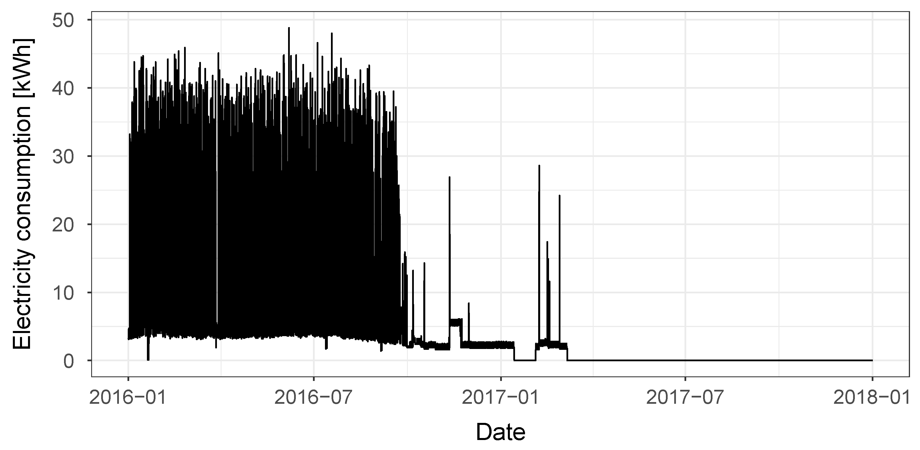


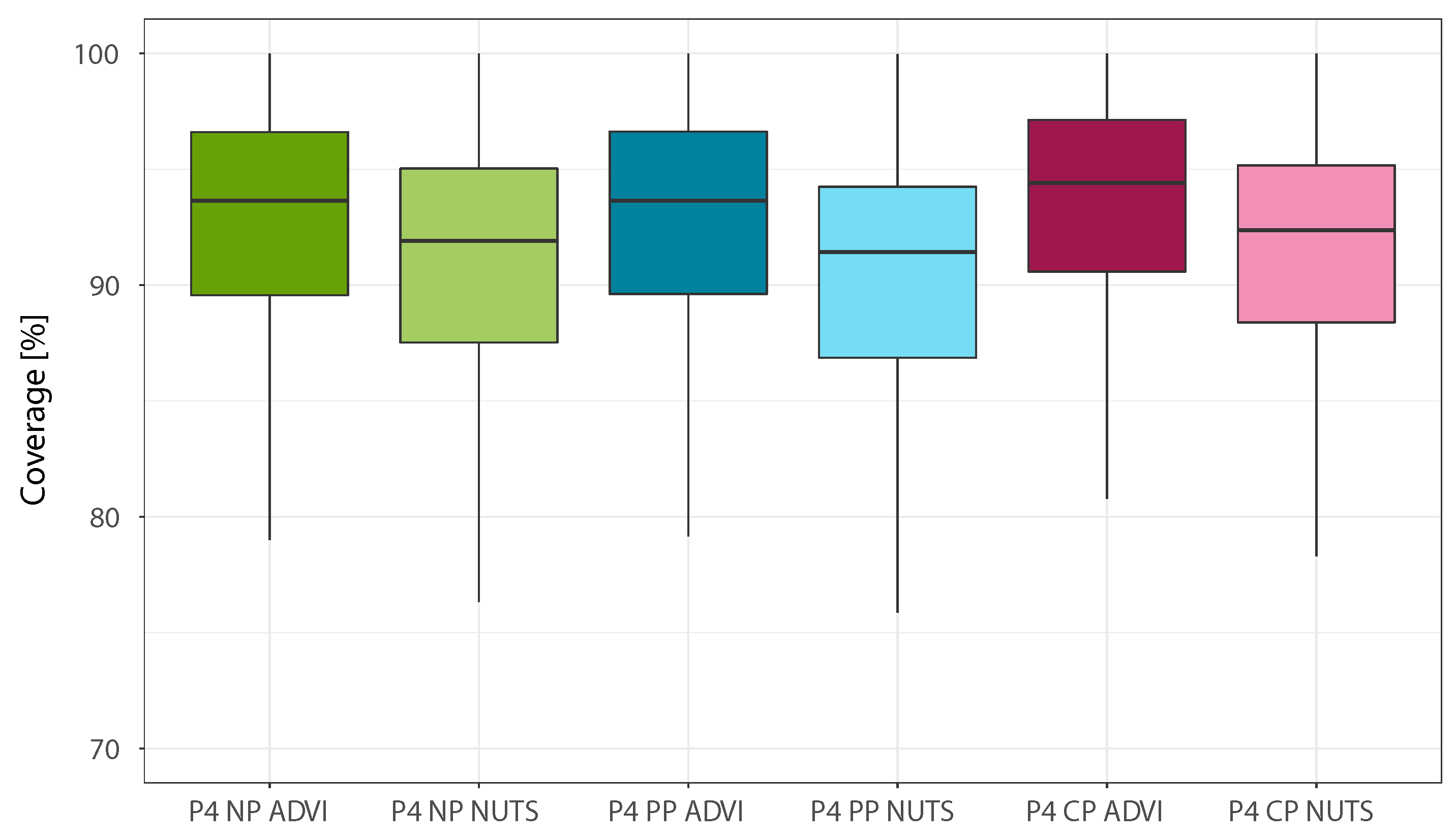
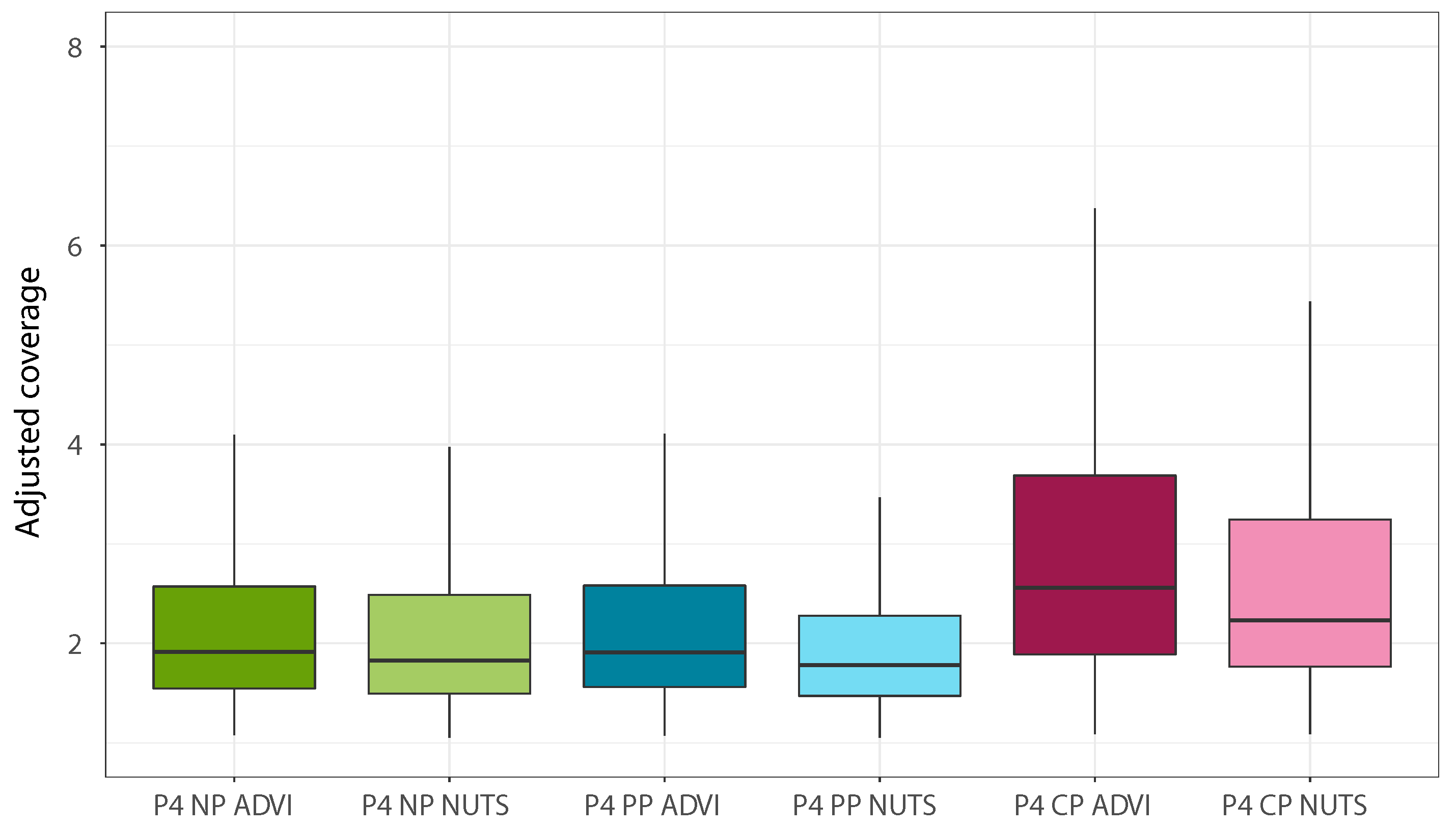


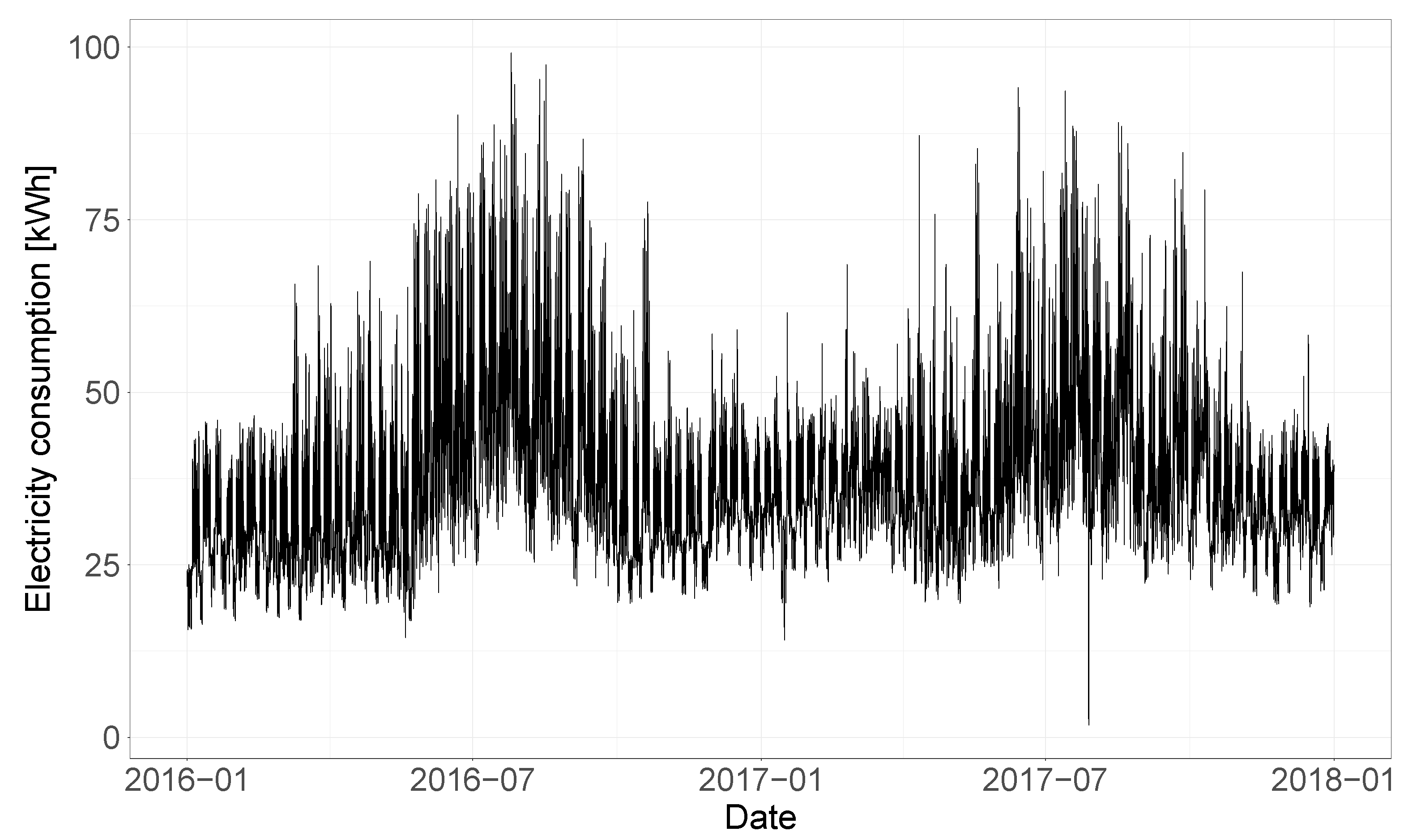
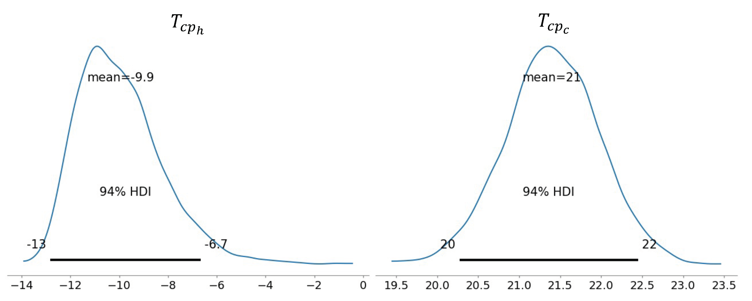


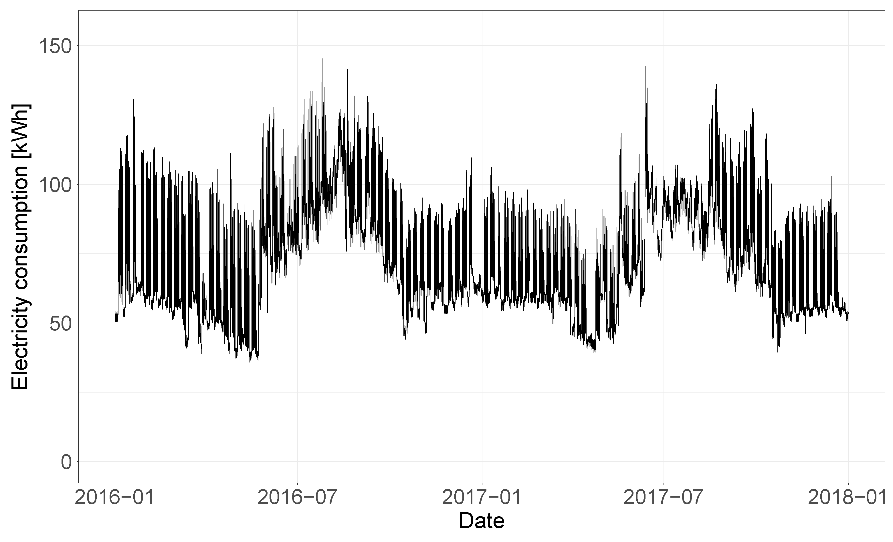
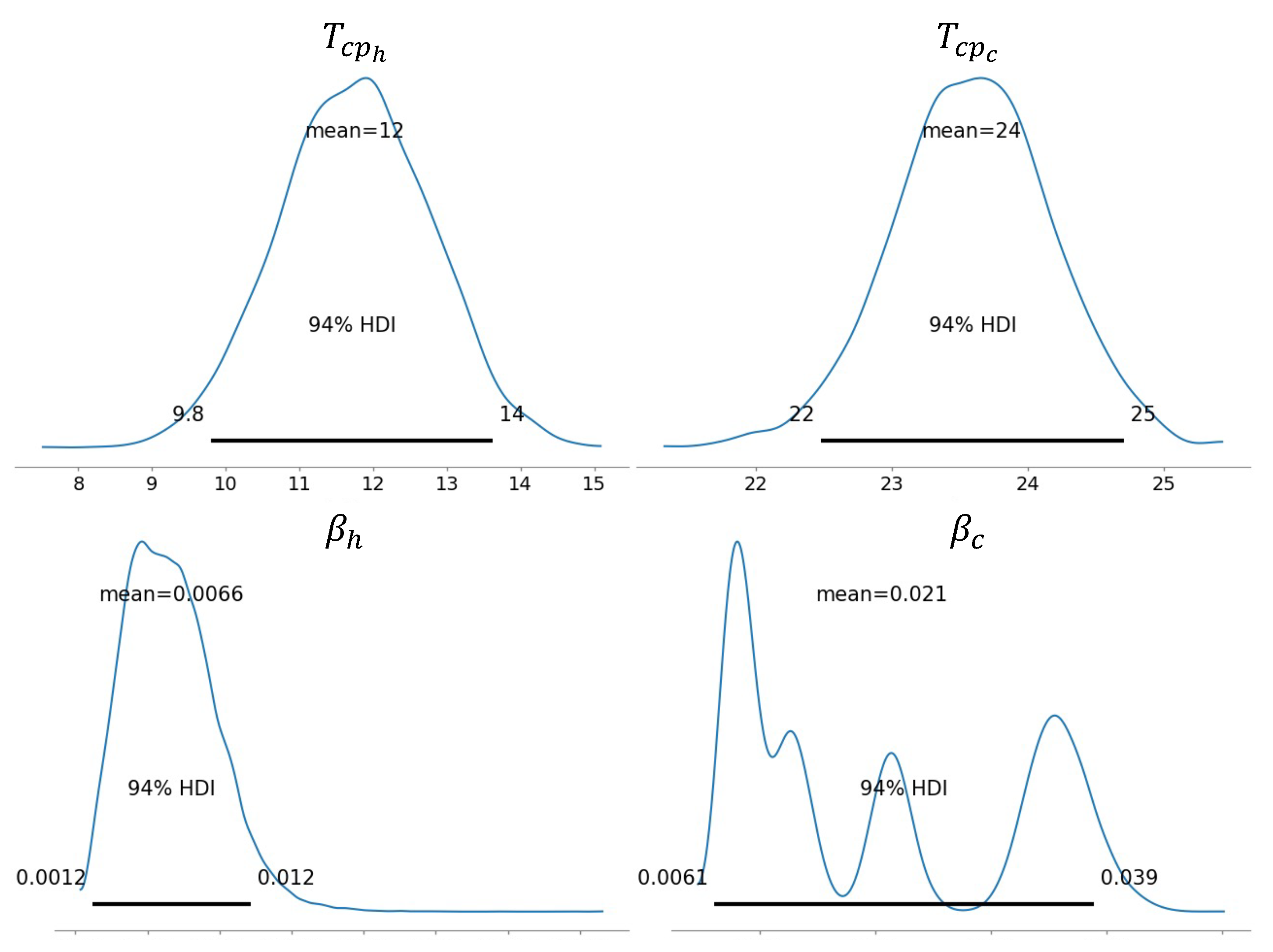
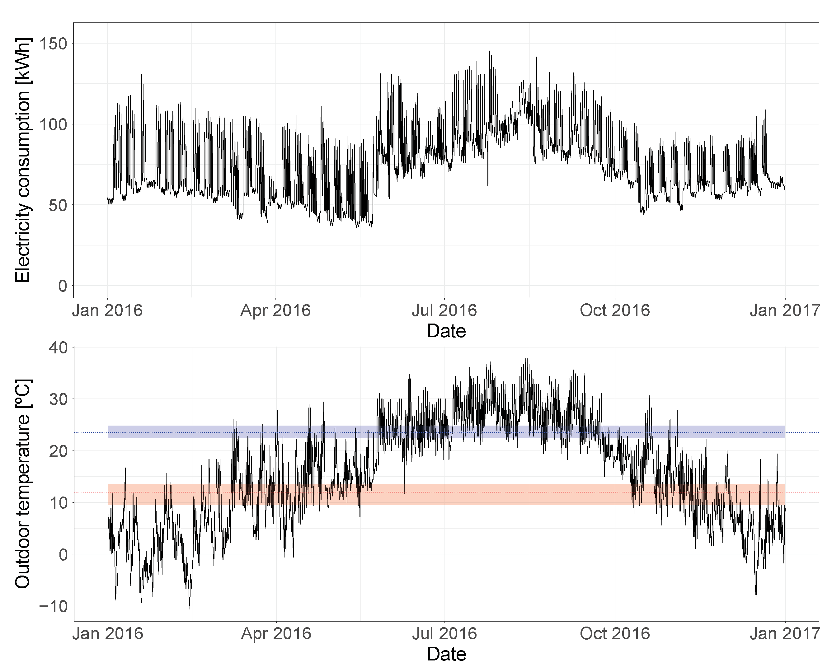
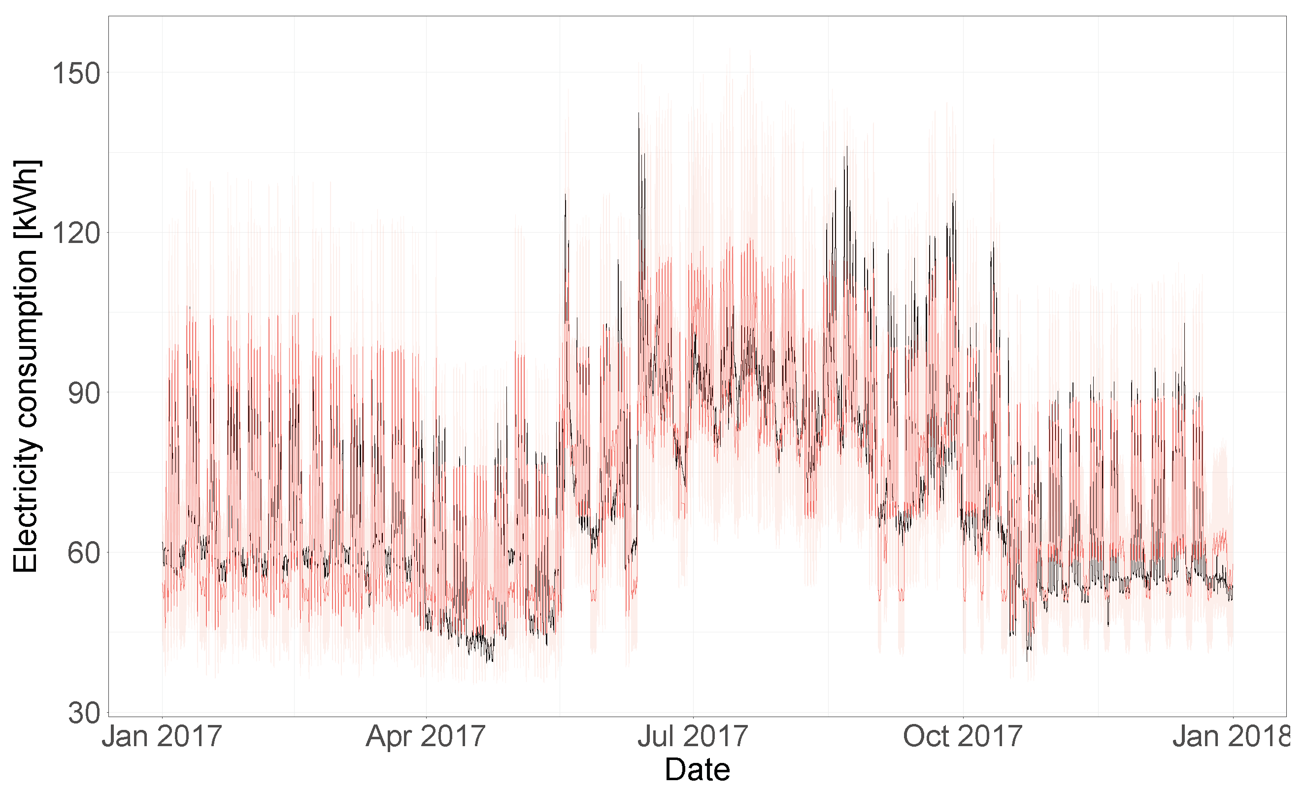

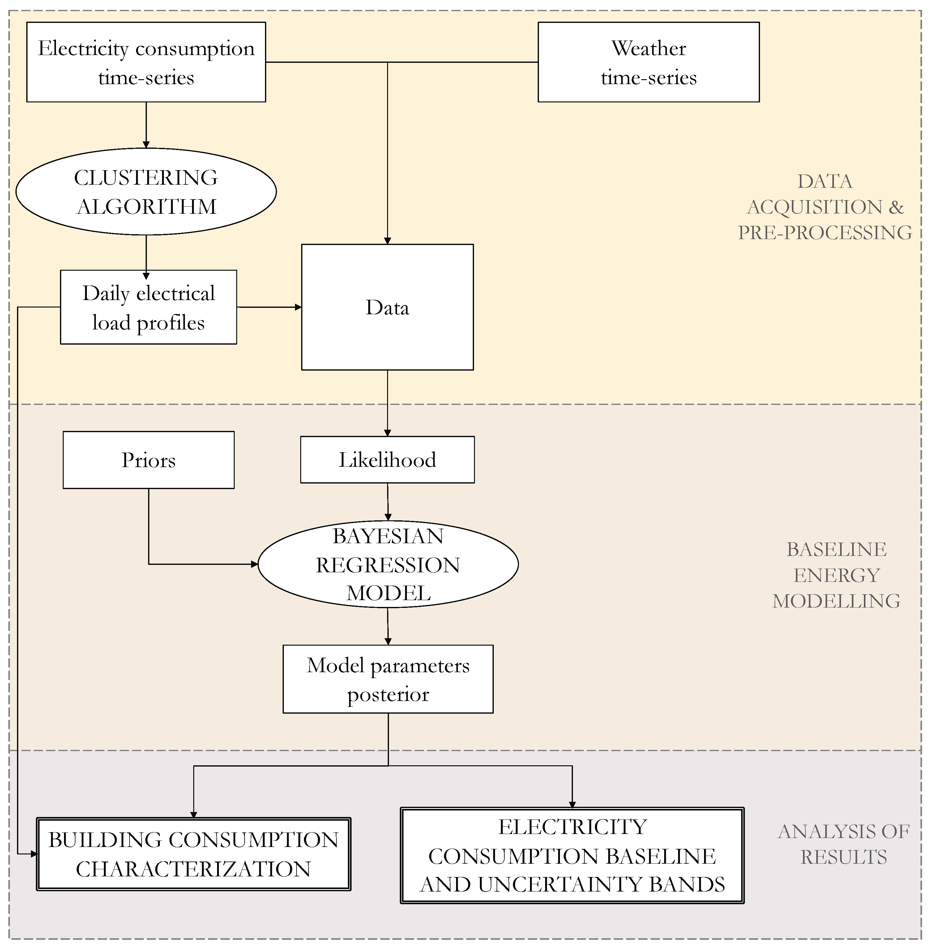
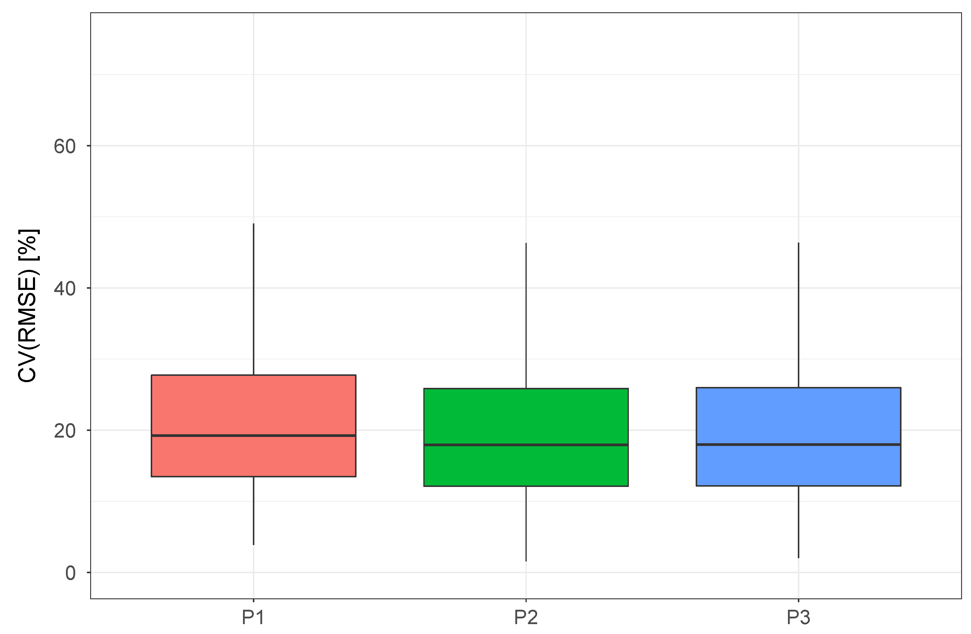
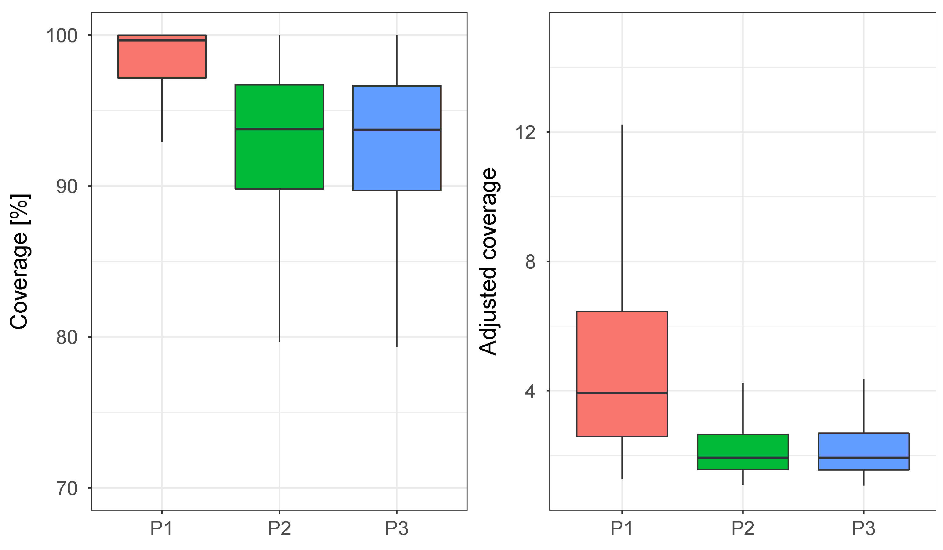
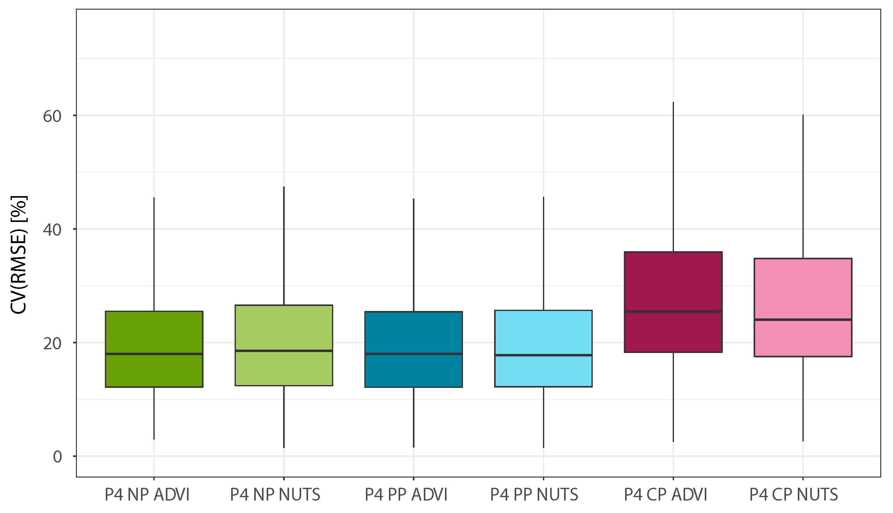
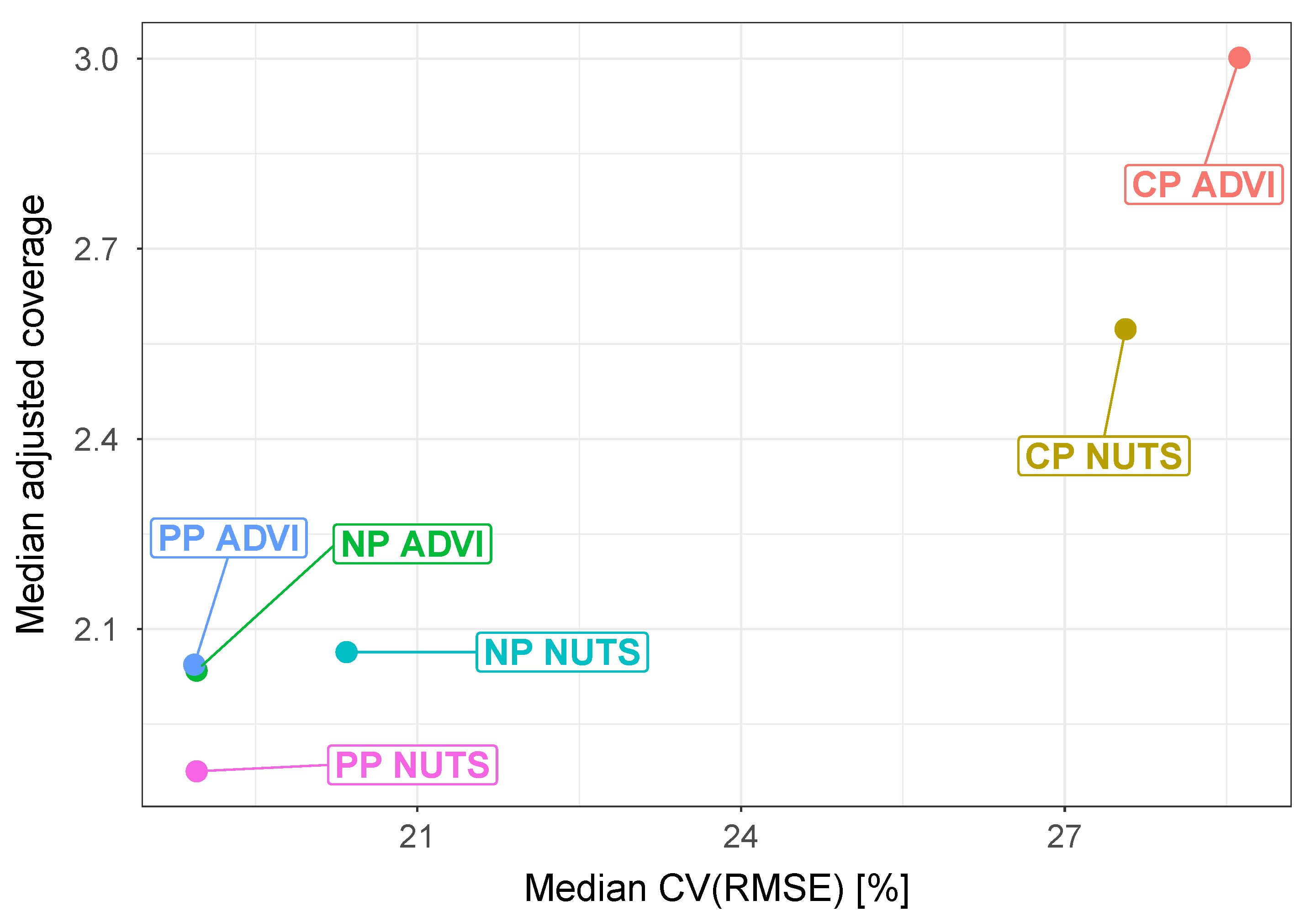
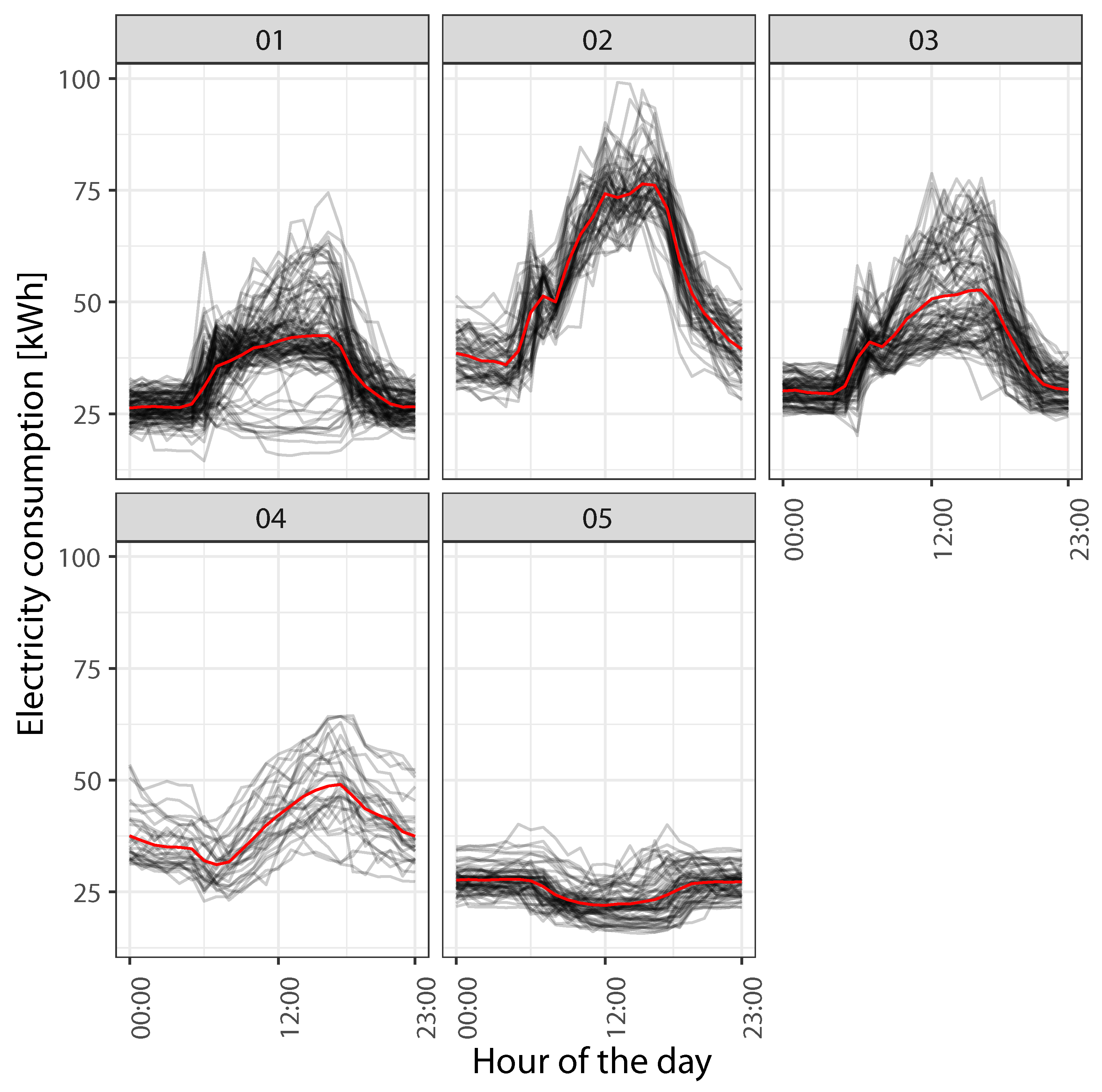
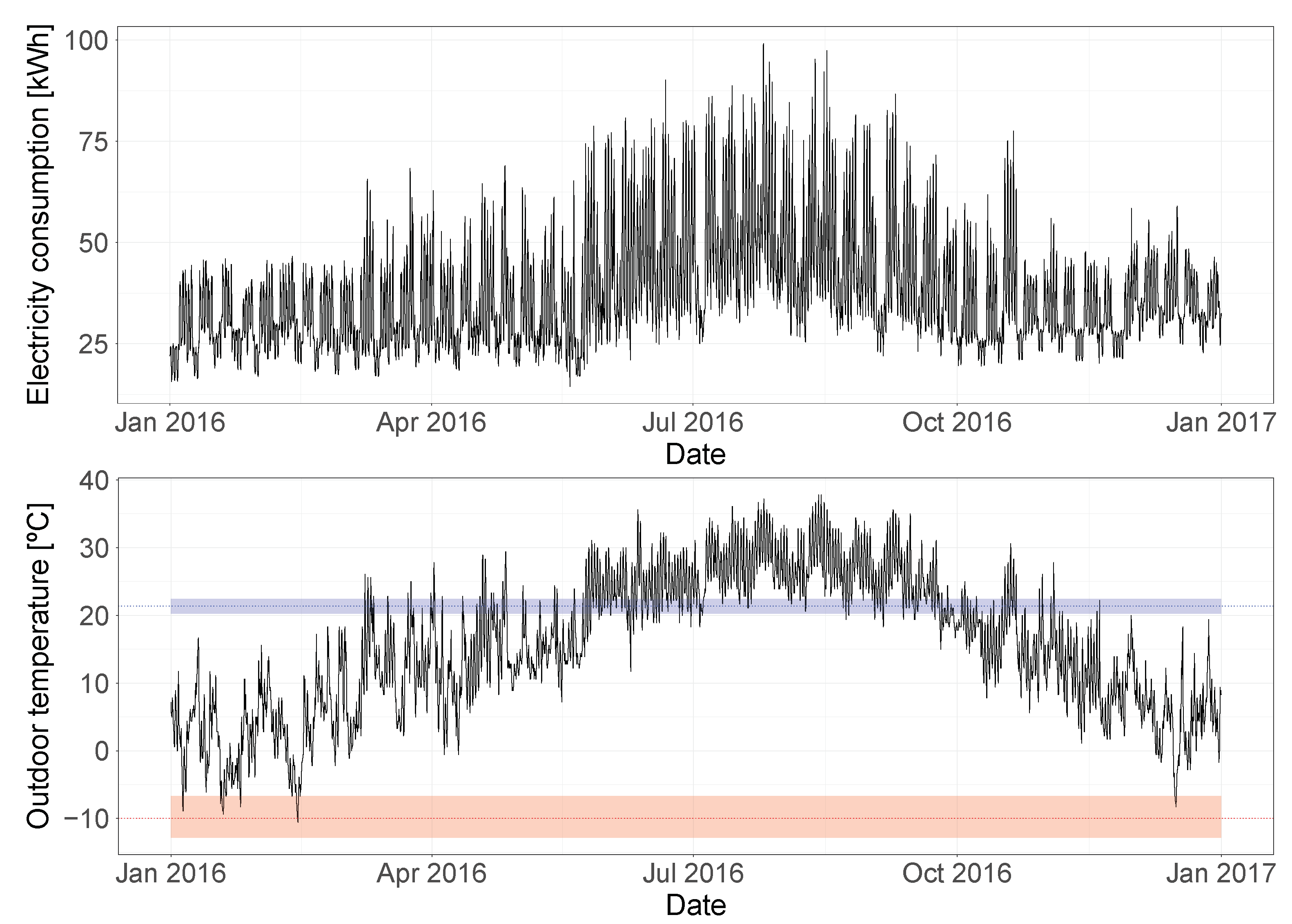
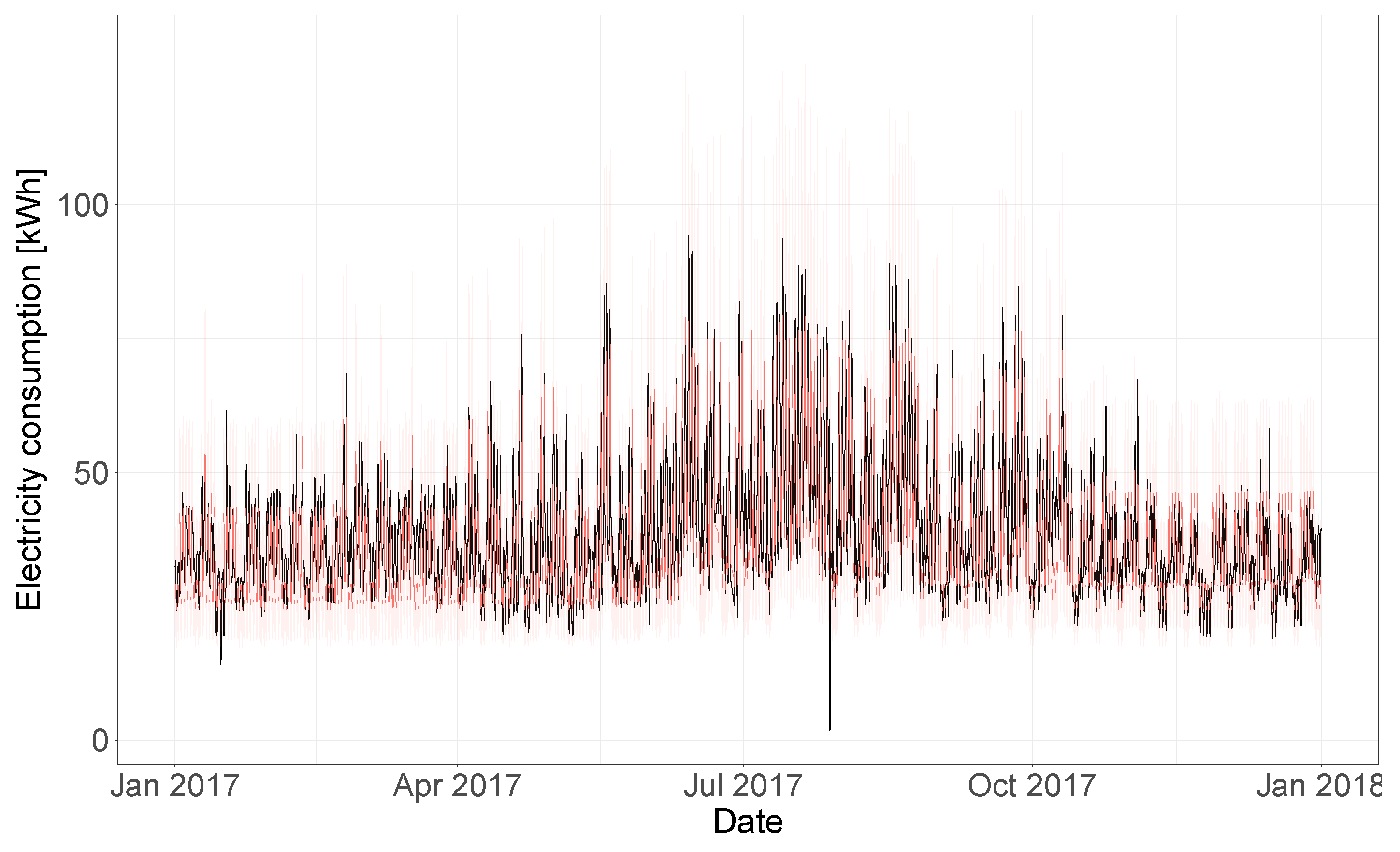
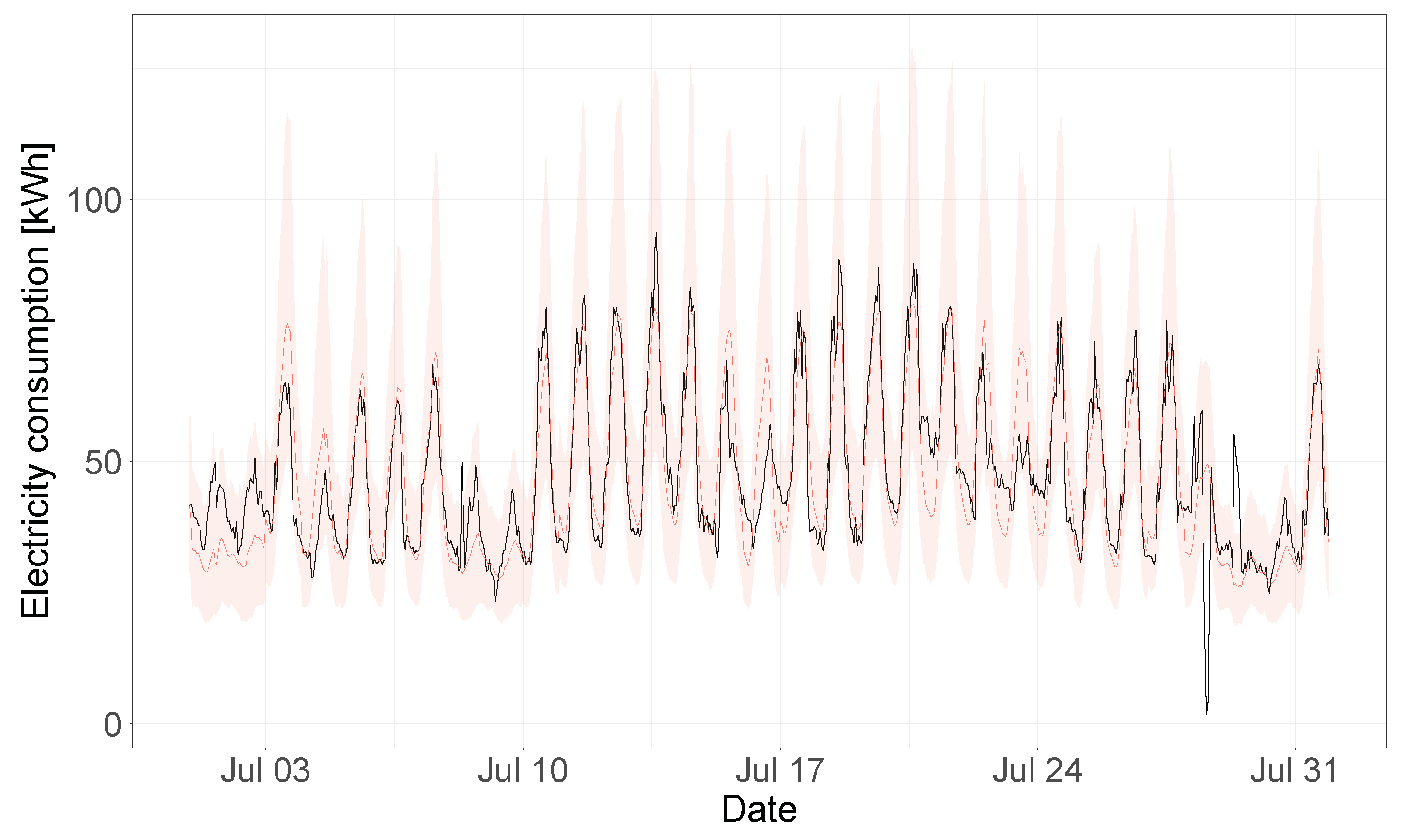