Article

Model for 400 kV Transmission Line Power Loss Assessment Using the PMU Measurements

1
Croatian Transmission System Operator, HOPS, 10000 Zagreb, Croatia
2
Faculty of Electrical Engineering and Computing, University of Zagreb, 10000 Zagreb, Croatia
3
Studio Elektronike Rijeka Ltd., 51000 Rijeka, Croatia
*
Author to whom correspondence should be addressed.
Energies 2021, 14(17), 5562; https://doi.org/10.3390/en14175562
Submission received: 2 August 2021 / Revised: 28 August 2021 / Accepted: 1 September 2021 / Published: 6 September 2021
(This article belongs to the Special Issue Advances in Synchronized Measurements Technologies in Smart Grids)

Abstract

:
This paper presents an advanced model for monitoring losses on a 400 kV over-head transmission line (OHL) that can be used for measured data verification and loss assessment. Technical losses are unavoidable physical effects of energy transmission and can be reduced to acceptable levels, with a major share of technical losses on transmission lines being Joule losses. However, at 400 kV voltage levels, the influence of the electrical corona discharge effect and current leakage can have significant impact on power loss. This is especially visible in poor weather conditions, such as the appearance of fog, rain and snow. Therefore, loss monitoring is incorporated into exiting business process to provide transmission system operators (TSO) with the measure of losses and the accurate characterization of measured data. This paper presents an advanced model for loss characterization and assessment that uses phasor measurement unit (PMU) measurements and combines them with end-customer measurements. PMU measurements from the algorithm of differential protection are used to detect differential currents and angles, and this paper proposes further usage of these data for determining the corona losses. The collected data are further processed and used to calculate the amount of corona losses and provide accurate loss assessment and estimation. In each step of the model, cross verification of the measured and calculated data is performed in order to finally provide more accurate loss assessment which is incorporated into the current data acquisition and monitoring systems.

1. Introduction and Motivation

Electricity losses in transmission networks can be divided into technical and non-technical losses [1]. Technical losses are caused by physical electrical effects, which can be divided into those originating from transmission line losses and transformer losses [2,3]. Non-technical losses are caused by unregistered and illegal connections, inaccurate measurements, and poor records of measurements, and it is impossible to determine the origin or the exact measure and location of these losses [4]. For high-voltage transmission networks, non-technical losses are negligible. In accordance with this, the dominant loss share in transmission networks is generated by overhead lines (OHLs). Electricity losses on transmission lines are caused by the known physical effects of the electricity current flow and can be divided into Joule losses, losses due to the corona effect and losses on insulators, with other types of losses being neglected due their insignificant amounts [5]. For the 110 kV voltage level, Joule losses are dominant, while on 220 kV and 400 kV lines, there is a significant influence of electrical corona discharge and leakage losses. This is especially visible in bad weather and high precipitation conditions [6]. Additionally, there is a significant error in loss calculation for OHLs, with low-loading due the equipment’s limitations in measurement voltage and current values [7]. The main goal of this paper is to assess the influence of corona and leakage losses through the development of the loss estimation model that utilizes phasor measurement unit (PMU) measurements.
There have been attempts to determine the influence of weather conditions on total losses in the transmission grid, where various methods have been applied [5,7]. All conducted analyses showed similar results, in that the amount of loss can significantly deviate among different 400 kV OHLs in relation to weather conditions and specific geographical influences. In some cases, the influence of weather conditions on the losses of 400 kV OHLs is such that ultimately, the losses caused by weather conditions occupy a dominant share of the total losses on 400 kV OHLs and can inherently cause significant errors in loss prediction [8].
The calculation of losses on transmission lines is presented as the difference between the sent and received power at two ends of the line. The calculation of the power in the transmission line is performed based on voltage and current measurements, and if the measurements are accurate, the calculation of losses is as well [7,9,10]. In general, existing estimation algorithms perform well when the measurements are accurate. However, in practice, changing the electrical and physical parameters of the transmission lines and the measurement equipment may contribute to errors in loss calculation. The main reasons for this stem from, e.g., measurement transformer saturation, non-transmission line synchronized measurements, data conversion errors or communication device malfunctions [7,10].
The conducted analysis adopted the approach of predominantly using statistical processing of historical measured data for each 400 kV OHL to determine the total loss and the annual occurrence of loss [10]. All performed analyses were conducted on measured data from electricity meters (ADVANCE for energy recordings) and SCADA systems (for various power system parameter recordings), which both represent the main systems in the management process of the transmission network. Both systems have certain shortcomings and limitations in determining the total loss and corona-related losses on 400 kV OHLs. Due to insufficient data from existing measurement systems and unprecise weather condition logs, it is difficult to exactly determine the types of loss. Therefore, further research on the availability of measured data was conducted, where measurements from PMU devices could provide a satisfactory level of accuracy and availability for the purpose of loss assessment. Measurements taken from PMUs were processed and used to determine the types of loss on 400 kV OHLs. The main advantage of PMU devices is the usage of synchronized measurements of current and voltage vectors needed to calculate losses. The values calculated in this way can be compared with the measurements from the ADVANCE system and compared to the expected theoretical values. In this way, calculated values are verified with measurements from various sources and can be used for the further purposes of determining losses on 400 kV lines with a greater confidence level [7].
This paper presents the technical background of the types of losses on transmission lines and the expected loss levels on 400 kV OHLs. Regarding the use of several measurement systems that are not standardized, the method of measurement data collection, data processing, data usage and data verification is presented. This method was performed according to the source type, and prioritization was conducted according to the accuracy. The calculation of losses on the 400 kV transmission line and the determination of individual components of losses from PMU measurements led to a better understanding of the types of losses and their amounts, as well as the dependence of losses (amount and occurrence) on weather conditions. In this way, robustness is achieved, which is very important, because ultimately, the calculated values will be used for market functions of loss procurement. To the best of the authors knowledge, this process and the usage of PMU data for the purpose of loss assessment, as was adopted in this paper, cannot be found in the state-of-the-art literature, and this presents the main highlight of this paper.
The main goal of the proposed model was to use a large set of metrics from different data gathering systems, ranking them with regard to their accuracy and reliability for the purposes of the better calculation of losses in real time. This was performed to develop a model for 400 kV transmission network loss assessment, with historical monitoring of losses for the entire 400 kV transmission network and real time calculation with day-ahead prediction included.
This paper is structured as follows: Section 2 describes the main aspects of high voltage losses, and Section 3 and Section 4 describe the way different data sources are used and combined in the proposed model. Furthermore, Section 5 deals with the influence that the physical aspects of high-voltage lines have on loss assessment, and Section 6 describes the importance of PMU measurements. Finally, Section 7 shows the results from the representative selected time frame. Section 8 and Section 9 conclude the paper, describing the applicability of the proposed model and providing the main conclusions and future work.

2. General Aspects of 400 kV Transmission Line Losses

The transmission of electricity from production (generation) sources to consumers inevitably causes power losses in all the elements of the electricity grid. As was already mentioned in the introduction, losses can be divided into technical and non-technical losses, where the dominant component of losses is technical losses, i.e., losses caused by current flow that are converted into thermal (heat) energy due to the resistance of the network elements. Non-technical losses are defined as an energy delivered but not metered or billed, and mainly occur in the distribution grid and are less impactful on high-voltage grids. Reducing losses, or at least keeping them at an acceptable level, is important from the technical, financial, and environmental points of view for all of the TSOs. A typical categorization of power losses is shown in Figure 1 [1].
Losses can also be classified considering their voltage levels, ownership relationship and different metering properties. In transmission systems, the dominant form of losses is technical losses, and they are, to a large extent, proportional to the loading of the elements. Due to higher voltage levels, it is expected in the transmission network to have lower currents and lower technical losses compared to losses in the distribution grid. It is also expected that due to the smaller number of total grid elements in the transmission grid, a metering point is available on each element of the transmission grid (lines and transformers), and losses can be determined in real time by direct metering, which is not the case for distribution systems. Figure 2 shows losses in transmission and distribution grids and their relative amounts according to different categorizations.

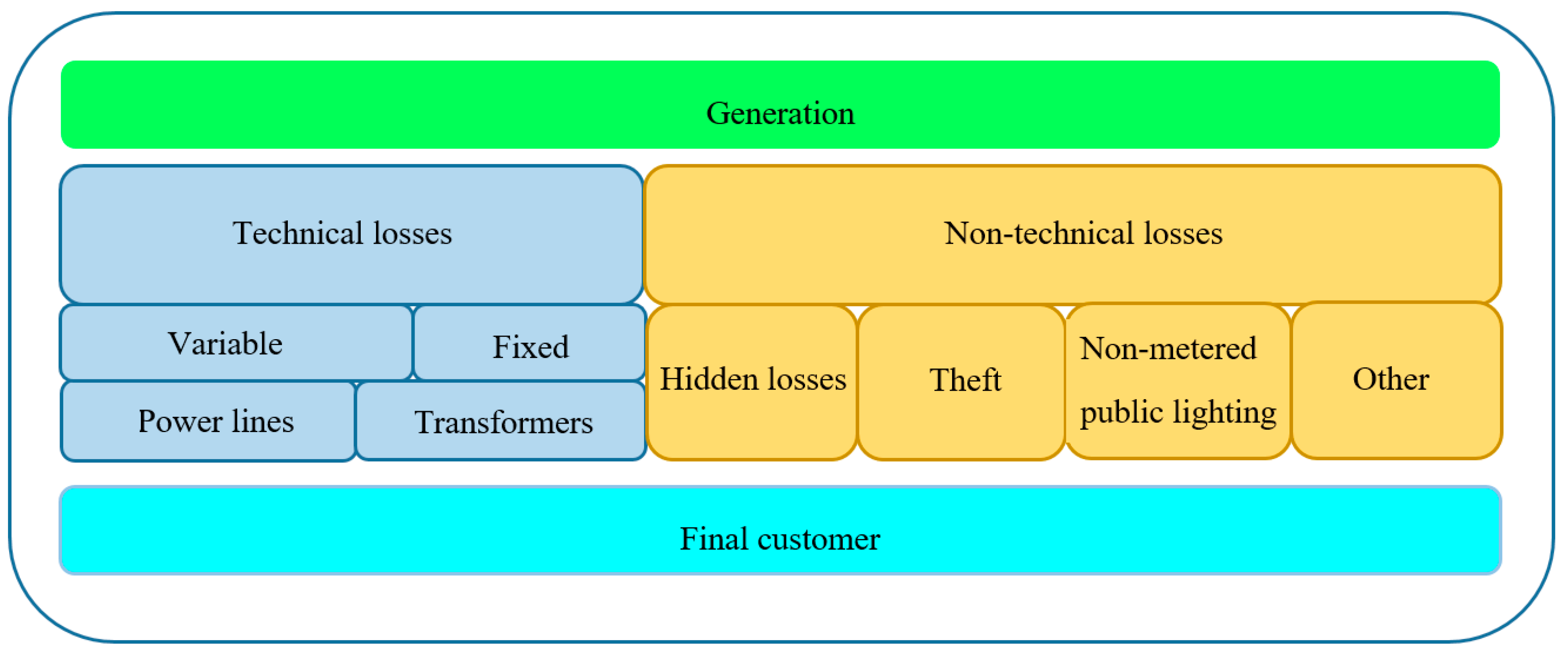
2.1. General Classification of Losses on Transmission Lines

Losses in the transmission grid can usually be determined by direct measurement. The most common method for calculating losses in the transmission grid is to calculate the power difference between the sending and receiving ends of the transmission line. Due to various technical limitations and economic reasons, the accuracy of measurements from lower-importance grid elements is not sufficient to determine individual losses. Therefore, this paper focuses on the most important (high-voltage) lines. Figure 3 shows the shares of losses in a transmission network. The majority of losses occur on lines, and they are approximately three to four times greater than losses from transformers.
Losses on transmission lines are mainly Joule losses caused by the conductor heating effect, which is proportional to the square of the current flowing through the conductor. To reduce long-distance power transmission losses, electricity is transmitted via high (or extra high)-voltage power lines, which typically range from 110 to 750 kV throughout the transmission network [1]. In addition to Joule losses on transmission lines, corona losses (conduction ionizes the air near the conductor) and leakage losses also occur. These losses are less significant and can be ignored at voltage levels below 230 kV [6,8,9]. However, due to bad weather conditions, corona and leakage losses can occupy a significant share of the total losses on 400 kV transmission lines, with the level of these losses being considered as a function of specific weather conditions.

2.2. Theoretical Background for Losess Calculation on Transmission Lines

There are several methods for calculating electricity losses from known electrical parameters in the system or estimating them on an experimental basis from measured data. The losses on the transmission line can be divided into Joule losses, losses due to the corona effect and losses from insulators (leakage) [10,11,12]. Ideally, for easier and faster calculation, the transmission line can be considered with symmetrical elements and can be presented as a single-phase element with concentrated parameters.

2.2.1. Joule Losses

Losses on transmission lines are mainly Joule losses (≈85%), as is shown in Figure 3. The total loss depends directly on the current passing through the conductors, and therefore the transmission losses can total up to ≈2–3% of the total power transmitted depending on the length of the transmission line. According to Equation (1), the Joule losses are calculated as follows [5]:
Δ P = 3 · R · [ P 1 2 + ( Q 1 U 1 2 · B 2 · 10 6 ) 2 3 · U 1 ] 2   ( MW )
P—Joule losses (MW),
P1—Active power on the beginning of the line (MW),
Q1Reactive power on the beginning of the line (Mvar),
U1—Voltage on the beginning of the line (kV),
R—Resistance of the line (Ω),
B—Susceptance of the line (µS).

2.2.2. Corona Losses

Corona losses occur when the voltage in conductors of the transmission line is higher than the critical electrical field value of the surrounding air, or when breakdown of the dielectric strength of air occurs. Consequently, the air is ionized, and energy losses occur. The amount of energy loss may vary from each case depending on: (i) line geometry, (ii) number of conductors, (iii) geographical position (altitude), (iv) atmosphere and weather conditions, etc. The determination of corona losses is mostly carried out on an experimental basis, and values are determined by the measured data. According to [9], it is possible to calculate the loss of the corona depending on the type and geometry of conductors. The calculation itself (expressed by Equation (2)) is limited by a set of parameters and satisfies the calculations for frequencies of 50 to 60 Hz [9]:
P k o r = 0.433 ( N r β ) 2 · l n 350 G M R · l n α G M R l n 350 α · P n     ( W / m )
N—Number of conductors
r—Conductor radius (cm)
β = 1 + 0.3 r Peeks factor
GMR—Geometrical mean radius
for N = 1 ≥   G M R = r
for N ≠ 1 ≥ G M R = N · r · A N 1 N
A—Radius of bundle
α—The mean distance of the spatial charge from the center of the bundle
for N = 1 ≥   α = 18 r
for N ≠ 1 ≥ α = 18 N r + 4
Pnfactor (taken from the diagram showing the power losses as a function of electrical field [9]).

2.2.3. Leakage Losses

Losses from insulators of transmission lines are not large during dry weather conditions, especially on newer power lines. On the other hand, on older lines, and in cases where pollution of the atmosphere along the transmission line corridor is significant, special attention is needed, because the insulation becomes imperfect and becomes very sensitive to weather conditions. In these cases, it is necessary to determine the possible amounts of loss from insulating chains when calculating total losses. Equation (3) allows the calculation of losses from insulators depending on the weather conditions [13].
P i s o = ( U 3 ) 2 n p R i s o   ( W / km )
U—Line voltage;
np—Number of insulators per kilometer of line length;
Riso—isolation resistance for a chain of insulator in good weather.
Losses from insulators at 400 kV voltage-level transmission lines are 3.24 times greater than the losses at 220 kV, since these losses are proportional to the square of the voltage of the power line.

2.3. Histroical Analysis of Losses in 400 kV Grid

Croatian TSO (HOPS) operates the 400 kV network in Croatia, which stretches throughout significantly different geographical routes. Since the 400 kV transmission network extends across the country with a variety of terrain configurations and with respect to the network transmission configuration and its impact/role, separate analysis was carried out for each transmission line based on gathered historical data. Given the characteristic periods of the year and according to weather conditions, separate analysis was conducted for the winter and summer periods. For the purposes of calculation and the estimation of losses, it was necessary to understand the method and quality of the data collected [10].
Table 1 presents the amounts of loss for different weather conditions and conductor configurations depending on weather conditions [5,14]. Comparisons of corona losses due to different weather conditions are given in Table 2. Due to bad weather, the amounts of corona loss can have a significant influence on the total loss.
According to the available research, the expected amounts for loss from insulator chains are shown in Table 2 [13]. For the observed 400 kV transmission lines in the HOPS network, the total losses during ice, rain and snow can be increased by 5 MW/100 km in total. The increase in losses is predominantly caused by corona losses (increase of 4 MW/100 km), while leakage losses contribute 1 MW/100 km [15].

3. Proposed Novel Method for Loss Assessment

The wide area monitoring system (WAMS) installed in the HOPS control center collects and processes synchrophasor (PMU) data in real time. There are ongoing activities in the continuous, incremental and gradual upgrading of the existing WAMS with new protection functions and control algorithms, aiming towards obtaining a wide area monitoring and protection (WAMPAC) system [15]. One of the implemented functions is line differential protection based on synchrophasor data. It was proven in practice that the new differential protection algorithm can be used as an effective tool for the validation of basic protection performance and as a solid foundation for the development and implementation of backup line protection [16,17].
The newly developed function of line differential protection was tested during our study on corona losses on high-voltage transmission lines. It was recognized that a real-time monitoring system provides the opportunity for gaining direct, continuous and timely insights into the system status and losses on OHLs. Measurements of current magnitudes and angles from the line, along with the PMU based differential protection algorithm, on a 400 kV transmission line were used to detect and estimate corona losses. Real-time testing of this function over the course of several months confirmed the validity of the concept’s usage for the recognition of corona losses.

3.1. Advanced Protection Functions of the WAMPAC System

The WAM system in HOPS collects synchronized measurements from all 400 kV high voltage transmission lines. The data are processed in a way that enables advanced protection functions to work in real time and enables the complete surveillance of faults or losses on protected lines. Line differential protection is implemented on 400, 220 and 110 kV transmission lines. The algorithm of this line differential protection is based on synchronized measurement data, comparable with relay protection device functions [18].
Furthermore, it gives insights into the operation of classical relay protection systems in the control room [19,20,21,22]. This also opens up possibilities to design other functions, such as a control function for corona losses which can be beneficial for the process of planning and the procurement of losses. The data flow is transferred to the WAMPAC system from each of phasor measurement unit (PMU) comprising 12 channels, with three phase voltage and currents measurements, including positive, negative and zero sequence of voltage and current [12].

3.2. Algorithm for Line Differential Protection

The transmission line protection algorithm is based on the calculation of the differential current—that is, the vector sum of synchronized current phasors at both ends of the transmission line. According to Kirchhoff’s law (Equation (4)), the vector sum of all currents in a closed circuit is equal to zero:
k = 1 N I k ( t ) = 0
The simplest configuration of instrument transformers is to place current transformers at both ends of the transmission line, at all three phases, where the current directions are set for the positive orientation of the current vector at both ends toward the transmission line (Equation (5)). Then, the vectors are ideally opposite in phase and equal:
I A f + I B f = 0
where I A f   is the vector of the current at phase f at one end and I B f is the vector of the current at phase f at the other end of the transmission line.
In practice, the vector sum of the current phasors will have an amplitude different than zero, caused by the loss of current due to the line’s resistance, while in the case of power line failures, there will be a large deviation before the protection is triggered. Line differential protection is based on the differential current of the transmission line Equation (6):
I d f = I A f + I B f 0
where I d f is the differential current of one phase of the transmission line. The line differential protection algorithm (Equation (7)) uses the amplitude of the real component of the current vector   I D f :
I D f = | I d f | = | I A f + I B f |
When the transmission line is energized from one end, the charging current   I c f of the transmission line is permanently present, which dominates the differential current of the transmission line (Equation (8)):
I A f + I B f + I C f = 0
For the purposes of the algorithm, a simplification was introduced that neglects the voltage drop on the transmission line, meaning that the voltage on the transmission line is considered constant. Then, a voltage from one of the ends of the transmission line can be used in the expression for the charging current of the transmission line. In the server algorithm, for the leading voltage, a side of the transmission line is selected, where, in the normal mode, the positive direction of the active power is measured, and the specified voltage can be used to obtain the impedance of the line shown by Equation (9):
I d f = I c f = U f Z f
where U f is the phase voltage at one end of the transmission line, I c f   is the phase charging current of capacitive character, and Z f is the impedance of the line with the majority of the capacitive character (Equation (10)), where X c is capacitive reactance—that is, X c < 0 :
Z f j X c
The amplitude of the differential current caused by the capacitive component is 5–15% of the amplitude of the rated current of the transmission line—that is, if there is no fault on the transmission line, then Equation (11) is valid:
I D o 0.15 · I n
where I n is the rated transmission line current and I D o is the amplitude of the differential vector in normal operation.
With a continuous charging current, large false differential currents can occur at higher loads or external faults, caused by transient saturation of current transformers. To reliably detect transmission line faults, the threshold for triggering an alarm is therefore defined by a curve that is a function of the sum of the amplitudes of the currents at the ends of the transmission line.
Given that such loads can cause differences in the measurements at the ends of the transmission lines, it is necessary to calculate the restrained current I R f , defined as the sum of the amplitudes at the ends of the transmission lines, Equation (12):
I R f = | I A f | + | I B f |
It is then possible to define the conditions for the triggering of the line differential protection depending on the magnitude of the differential current amplitude I D f , the magnitude of the restrain current I R f , and their mutual ratio.
The load curve of the transmission line load is typically divided into three sections according to Figure 4. The first section of the protective device tuning curve is defined by the minimum limiting value of current which cancels out the influence of the charging current, I D m i n , and the ultimate limiting current of the first section I R s 1 .
The usual value of I D m i n   is 30% of the rated current, which suppresses the sum of the two amplitudes of the previously mentioned transmission line charging current by a maximum of 15%.
In the second section of the curve, a linear dependence on the magnitude of the limiting current (Equation (13)), s l o p e s 2 , is added to the limiting current   I D m i n .
s l o p e s 2 = Δ I D f Δ I R f · 100 %
The third section has a slightly higher slope in practice, as shown in Figure 4a. The conditions required for triggering the protection in the WAMPAC module for the whole characteristic are shown in Figure 4b.
Losses on OHLs are calculated as the difference between the sent and received power at two end of a line. When the total losses are known, the calculation of Joule losses is performed. The calculation of Joule losses is conducted based on the range of temperatures that are measured or, in the case of unavailability, selected from historical measurements. From these calculated values, PCorona is expressed as the difference between total losses and Joule losses, as shown in Equation (14).
P = P J o u l e + P C o r o n a
Corona losses are represented by the current I d f , where I d f is the differential current on one phase of the transmission line. When a corona occurs, the differential current is unchanged, but the differential current angle changes slightly on the transmission line, and so corona is presented as an additional differential current with a different angle, and is expressed in Equation (15) as a function of the angle.
P C o r o n a = f ( a n g ( I d f ) )
Vectors of the current and voltage and their relationship are shown on Figure 5. I A   is the vector of the current at phase f at one end, and I B is the vector of the current at phase f at the other end of the transmission line. As was mentioned previously, the differential current is expressed as the difference between the I A f current and the I B f current.

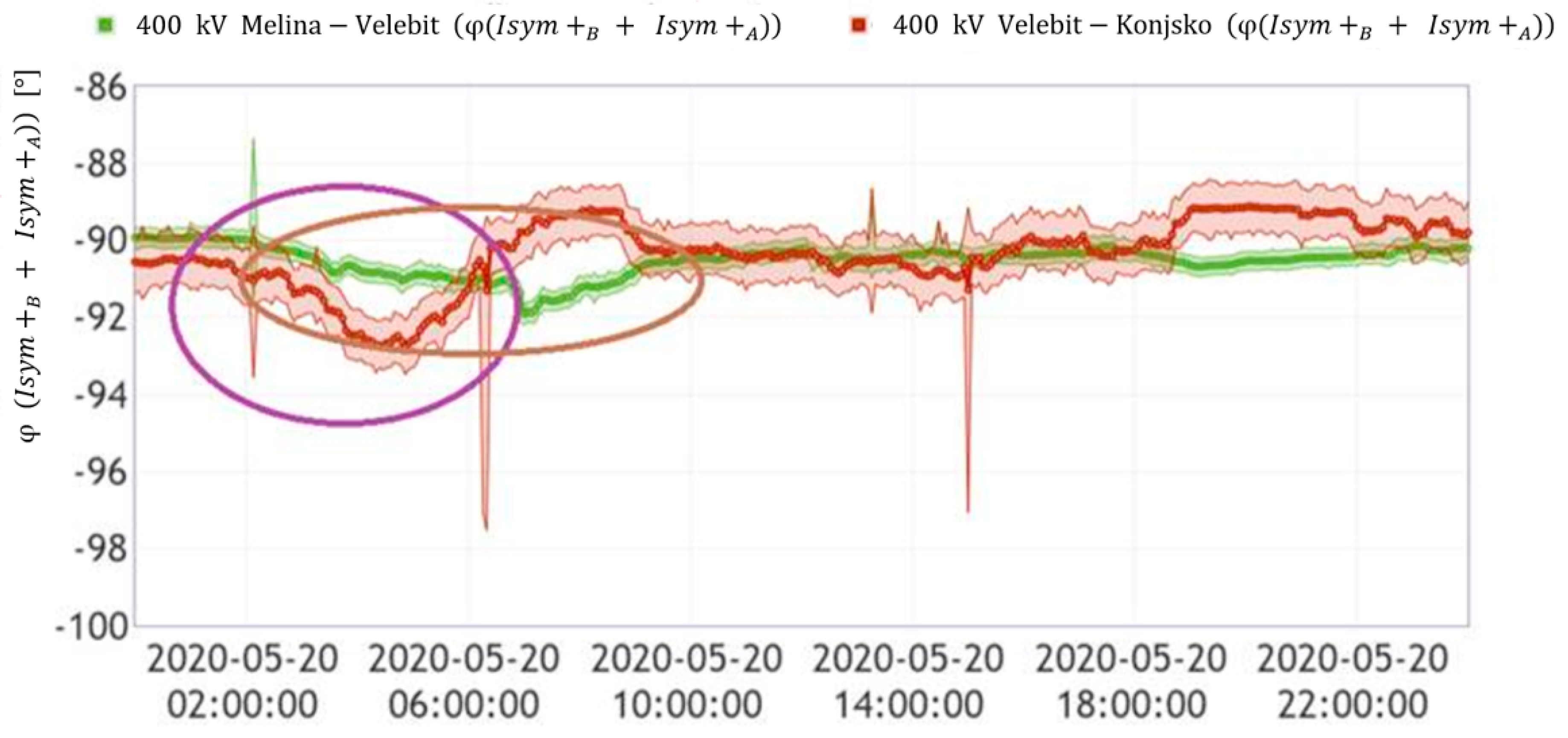
3.3. Corona Conditions on 400 kV Line Recorded by Line Differential Protection Using PMU Meassurements

During the conducted analysis of corona losses, many different operational conditions were investigated, and data from systems applications in the control room were analyzed. The conclusion was that PMU data can provide an excellent source of measurements, and these data are synchronized and available in real time.
In the first stage of this analysis, 10 min values of harmonics were obtained and detailed analysis of waveforms was conducted. It was concluded that their correlation with the total corona losses is very low.
Consequently, the second stage of the analysis extended to the datasets that included changes in differential currents on both ends of transmission lines, which were calculated using PMUs. Small adjustments needed to be made to the logging function, and it was extended to also monitor the angle of the differential current and compare it with the average voltage value at both line ends. In the ideal case, this angle should be close to 90°, as shown on Figure 6. This characteristic was found to be appropriate for use as an input for the loss calculation model, since it has a direct dependency and high correlation with the occurrence of the increase in corona losses.
The correlation between corona losses and the values of the angle of the differential current is expressed in all moments when deviation from the default angle of 90° is present. Figure 6 presents conditions on two 400 kV lines for the differential current with the magnitude and angle.
Compared to good weather conditions, heavy rain was recorded for the transmission line corridor of Konjsko-Velebit-Melina. For that particular day, it can be seen that the differential current angle value reaches 92°, which strongly indicates a high increase in corona losses. In this case, the differential current angle reaches values of 94° (purple circled area on Figure 6) in the period of heavy rain and large corona losses in the observed transmission line corridor (Figure 7). The correlation of the current angle value with the total corona losses is significant and can be used to determine the number and time of corona occurrences.
This is an example of the strong correlation between the monitored parameters, the differential current angle and the corona losses estimated from metering device systems. This refers to the occurrence of the corona, which greatly coincides with the deviation of the measured differential current angle from the normal operational conditions. These normal operation conditions assume the angles to be close to 90 degrees. Similarly, for the 400 kV line Melina-Velebit, there is an angle value deviation of 2° due to the occurrence of corona losses, compared to usual operating conditions under good weather conditions. Furthermore, this is strongly correlated with the occurrence of rainfall, and this aspect of the described model is further discussed in Section 7.

4. Proposed Model for Collection and Processing of Data and Calculation of Losses

To establish a model for loss calculation, basic technical features and mathematical models need to be developed. The main segments of the proposed model include the data collection required for loss calculation functions:
  • measured load on the OHL;
  • historical data on the OHL;
  • comparison of estimated and measured data;
  • monitoring of the element efficiency of the network;
  • weather conditions measurements;
  • historical data for each line separately;
  • analysis of measured data and statistical error and detection of measurement errors;
  • measured and calculated/estimated data on lines from historical data depending on weather conditions.
All of the abovementioned functions allow for the better and more accurate prediction of losses. The proposed process of calculating losses is an iterative process that uses existing measured primary data from electricity meters and PMU devices and compares them with historical data. A more detailed description of the process and proposed model is given in the following chapter.

4.1. Data Collecting Functions of the Proposed Model

The existing system for the collection of the measured data in the transmission network comes from various devices that are connected to current and voltage instrument transformers. The systems that measure and collect electrical data and their main features are listed below.

4.1.1. Electricity Billing Meter Data (ADVANCE)

Electricity meters are connected in two ways to the existing metering systems. The older meters are connected to the data logger (FAG) via pulse inputs or via communication. New electricity meters can communicate directly with the server. The basic functions of the software system are the collection, validation, storage and processing of metering data for billing purposes and other operational processes. Their monitoring functions provide the possibility to detect disturbances in the collection and registration of billing measurement data.

4.1.2. PMU Device Data

PMU devices are connected to voltage-measuring transformers (secondary winding for measuring) and to current-measuring transformers (secondary winding for measuring or protection). The block scheme of the WAM system that gathers PMU measurements in the Croatian transmission network is presented in Figure 8. Measured data from transmission lines are sampled at a frequency of 20 ms. Real-time data are collected (with the delay being a few tens of milliseconds) and are stored in the central database. In this way, the data can be used for advanced applications in the processing of losses, which is especially interesting for internal 400 kV transmission lines, because they are all covered with PMU devices at both ends of the OHL.

4.1.3. SCADA System Data

Power measurements are integrated at the SCADA system level to calculate energy measurements for the required secondary source in the reports. The measurements of the mentioned physical quantities in this are, as a rule, less accurate and reliable than energy measurements from electricity meters. For SCADA measurements, the core of measuring transformers is an accuracy class of 0.5. The accuracy of the measurement depends on the type and age of equipment of remote monitoring and control equipment, as well as on the set dead zones and the refresh parameter [23,24].

4.1.4. Power Quality Monitoring Systems Data

Power quality monitoring systems are designed based on digital devices that allow measurements of required electrical values such as voltage (phase and line), current by phases, frequency, power factor, higher harmonics, active and reactive power and energy. The devices enable the recording and analysis of waveforms and transients, harmonics analysis, display of phasor diagram, voltage and current imbalance, etc., which are all useful inputs for designing the model of loss calculation [25].

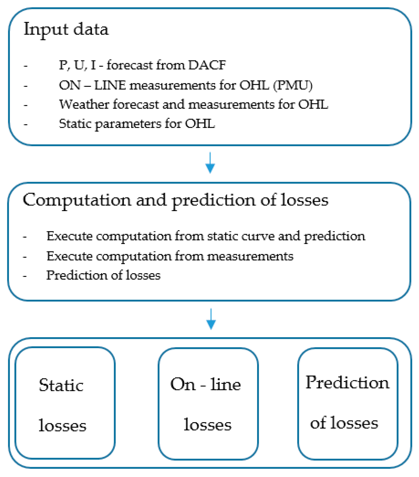
4.2. Losses Calcuation Function of the Proposed Model

All measurements of electrical values of the transmission network are taken from current and voltage measuring transformers and collected in the existing system. Measuring devices are connected to measuring transformers, with the aim being to measure, calculate and store the main electrical values. For the purposes of determining electricity losses, due to the characteristics (speed of response and arrival of metering data, and the accuracy of the data itself) of existing measuring systems, electricity meters and phasor measurement units (PMU) are predominantly used.
To assess the losses on 400 kV OHLs, several models for calculating losses were developed with regard to the possibility of data collection and processing them. Figure 9 shows the modelled steps for calculating and comparing the calculated losses. In the first step, input data from various operating and measurement systems are taken. From day-ahead congestion forecasts (DACF), the calculated values of currents, voltages and power flow are taken for each transmission line. In addition to these data, measurements from the PMU devices are taken as the primary source, and data from meters and SCADA are taken as a secondary source. Additionally, weather forecasts and measured weather data conditions are taken, which include temperatures, type and amount of precipitation and humidity. The calculation of losses for each transmission line is performed based on the collected data. The first step in the calculation of the losses on OHLs is performed based on the values from DACF calculation. For each OHL, the ohmic resistance of the conductor is taken as R20 °C (ohmic resistance at 20 °C). During the ongoing day (24 h), losses are monitored through the existing measurement systems (measured data from electricity meter and PMUs). In cases when weather conditions change, and accordingly weather forecasts predict significant changes in temperature, rain, snow, etc., the replanning of losses is conducted for each 400 kV OHL. Through the performed calculation, deviations of flows and losses along transmission lines can be easily noticed. Changes in power flow in the transmission network in most cases come as a direct consequence of a change in the production/generation schedule, unplanned exchanges with neighboring TSOs, or as a consequence of the new topology of the network. Due to the change in power flows, a change in losses is to a smaller extent related to planned losses. In conditions with heavy snow and ice, a significant level of loss can occur in the transmission network, especially at 400 kV. The planning of additional losses is performed within the day using the most recent weather forecasts. The final results are the values of the initial/static day-ahead loss calculation, on-line loss measurement values and loss projections for the period until the end of the day (24 h period) including the assessment of the type of losses, namely corona losses. The described algorithm can be used in the daily routines of the TSO for the purposes of planning and replanning losses (adjusting the initial plans). In this way, the existing loss planning and purchase process is improved, better accuracy of loss planning is achieved, and the financial cost required to cover losses on the intraday market is reduced. Furthermore, data collected in this way can be used in the process of understanding losses on transmission lines, especially at the 400 kV voltage level.

5. Model of 400 kV OHLs for Loss Assessment

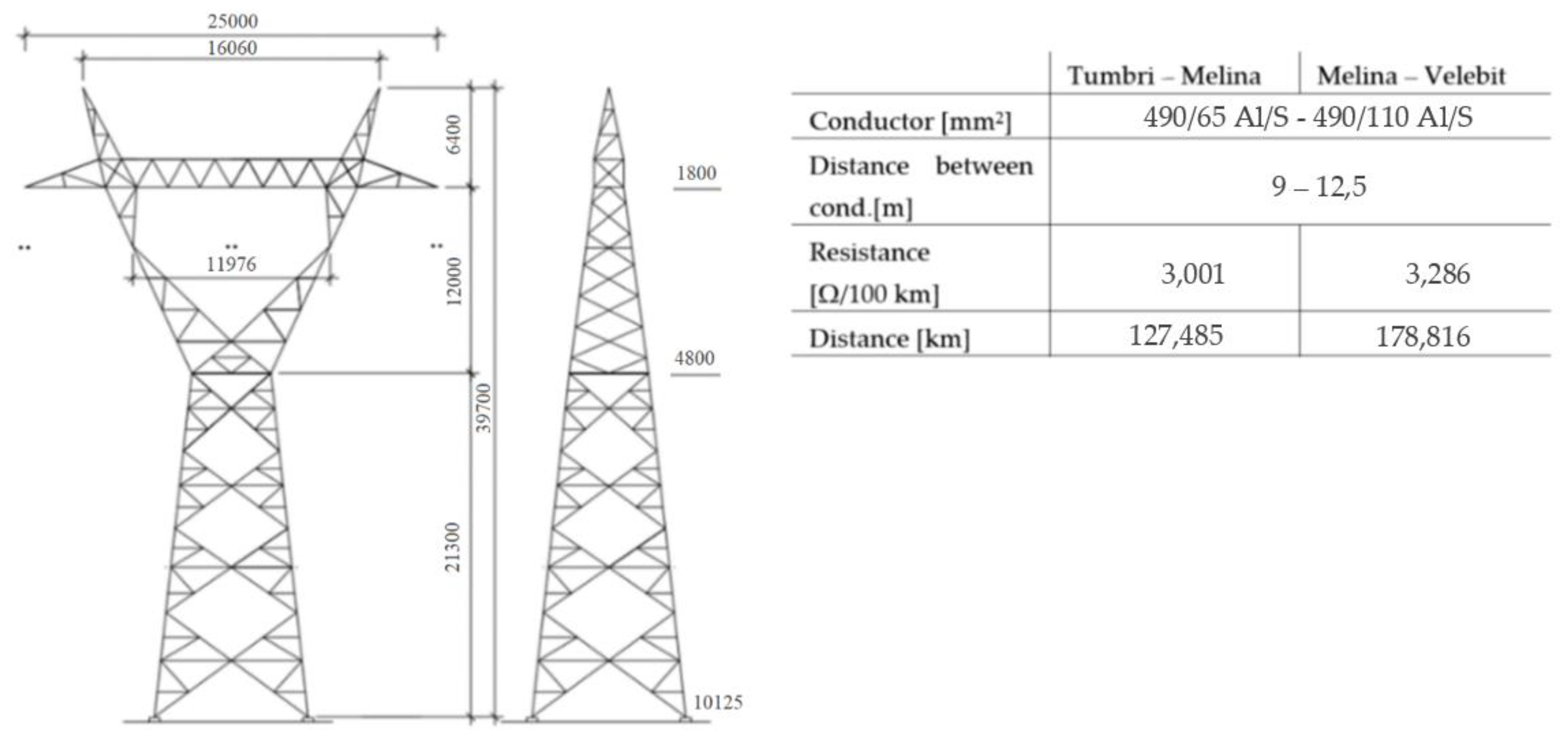
5.1. Croatian 400 kV Transmission Grid Main Chacteristics

The Croatian 400 kV transmission network is not entangled within the Croatian territory, but extends from the eastern substation (SS) SS Ernestionovo to the central part (SS Žerjavinec and SS Tumbri), to the west (SS Melina) and south (Velebit and Konjsko). The reason for this wide reach is that the Croatian 400 kV transmission system was built as the backbone of the transmission system of the previous country, Yugoslavia, with the focus being on strong interconnections with transmission systems in the area to BIH and Serbia, and due to the geographical characteristics of the Croatian territory. The Croatian 400 kV transmission grid is shown on Figure 10, where the three main 400 kV lines that are the focus of this model’s development can be observed.
Most of the 400 kV transmission lines are 30 years old and older. The first of the 400 kV transmission lines, including lines in the Konjsko-Velebi-Melina corridor, were designed and built on steel lattice poles with a “Y” head shape. For the conductors, aluminum of a nominal cross section of 490/65 Al/S mm2 was chosen, with two conductors in a bundle per phase (3 × 2 × 490/65 mm2 Al/Steel). Insulation chains composed of glass-capped insulator cells with an installation height of 170 mm were used for the insulation of the transmission line. Since the physical characteristics of the OHL play an important role in corona losses due to different electrical field gradients between the lines caused by the different physical layout and design of its components, the main types of poles and conductors that are observed are depicted in Figure 11 [15]. The Croatian 400 kV transmission grid extends across the country, with a variety of terrain configurations and with similar tower configurations and conductor configurations in each corridor. Therefore, it is possible to perform the analysis of the impact/role of geographical terrain and altitude on each transmission line based on the historical data.

5.2. Losses Calculation in Existing Metering Systems

Losses are calculated on multiple levels to achieve better accuracy and robustness in the system in its daily operation. Losses are calculated separately for the whole 400 kV transmission grid and for each 400 kV OHL individually. The system is designed to recognize the status of measurements, amounts and sources of data. With this approach, it is possible to perform further analysis to assess the types of losses and the occurrence of an increase in losses due to, for example, corona, within a daily/weekly/monthly period. Figure 12 shows the losses on an hourly basis for a month-long period (May 2020) for the observed 400 kV transmission grid. The same analysis is performed for total losses and corona losses for each 400 kV OHL separately, and detailed analysis will be provided later (Section 6).
To better understand the levels of losses and their interdependence on load flows and weather conditions, it is necessary to make a comparison between on-line measured data and historical measurements. Figure 13 shows the load flow (blue line), measured on-line losses (red line) and estimated losses (green for summer and purple for winter periods). A good match between on-line losses and estimated losses can be observed most of the time, except on 20 May 2020 in the morning hours, which is discussed in Figure 6. This provides further motivation for this work and for the further development of improved models for loss estimation, since, for that and similar periods, it is necessary to perform additional analysis to obtain a better understanding of the causes of these increases in losses.

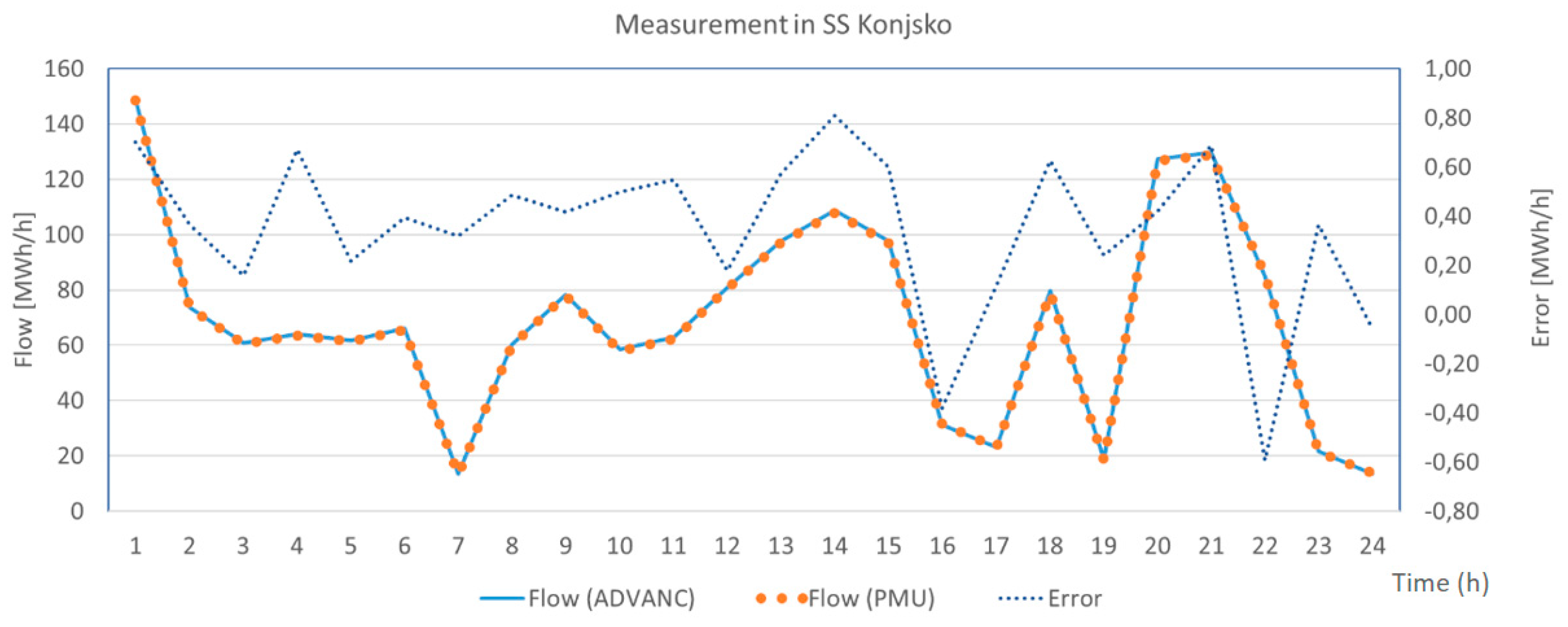
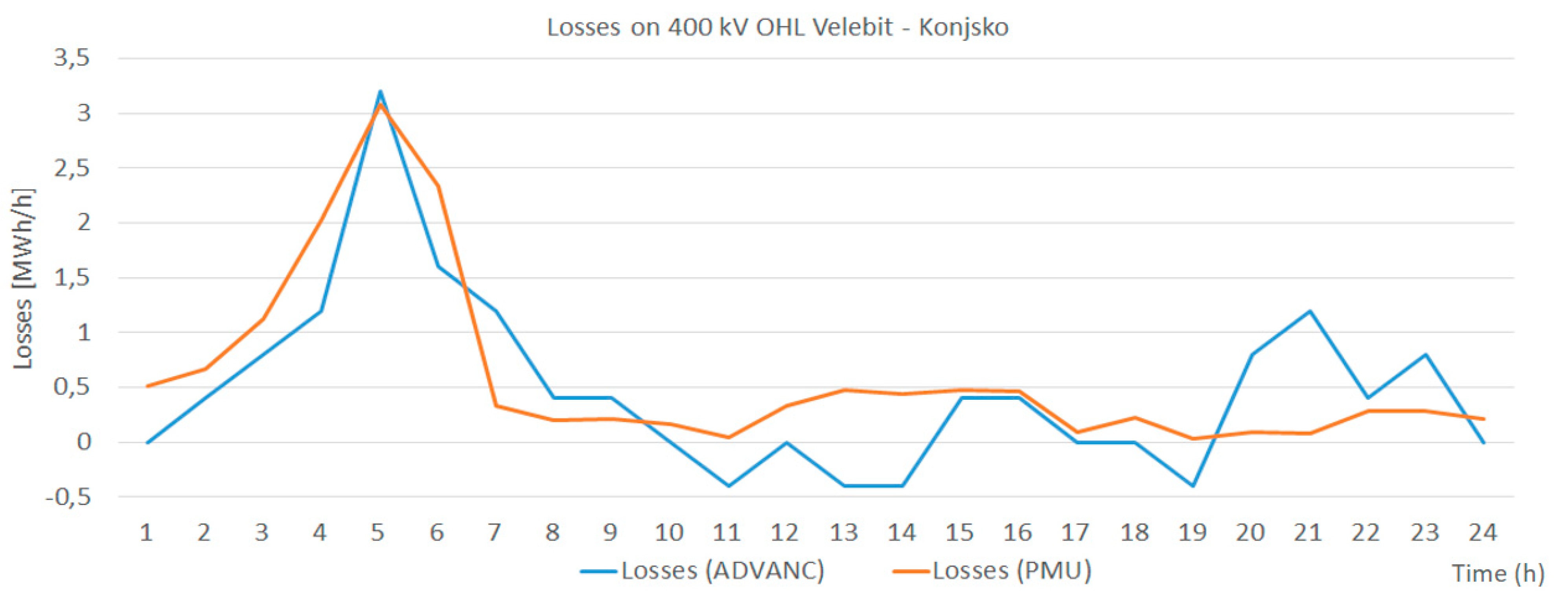
5.3. Loss Calculation with PMU Measurements

To successfully determine individual types of losses on each transmission line, PMU measurement data were utilized. The measurement data were collected with identical PMUs on both sides of the OHL. An angle measurement error of 0.01%, a current measurement error of 0.03% and a maximum relative voltage measurement error of 0.02% were accounted for.
Existing programs and applications for monitoring components and losses on transmission lines from PMU measurements are very sensitive to the quality of voltage and current measurements, i.e., the amount of error that the measured quantities contain. Most of these errors come from the measured transformers, while for system errors, it is possible to perform an estimate based on the calculated results [10,11]. In Figure 14, the differences in power flow measurement taken from ADVANC and PMU measurement on both sides of the OHL can be seen. The main cause of the shown difference is the different methods of measurement from the PMUs and the ADVANC system. A detailed analysis of the uncertainty of the calculated measured values is also taken into account.
It can be seen from Figure 15 that measurements from the PMU and the ADVANC system are related to the measured values. From the PMU and ADVANC measurements, losses are calculated as the difference in flows between the substations at both ends of the line. What can be noticed is a negative amount of loss from ADVANC measurements, which can be explained because the measurements are not synchronized and errors from measurement transformers are unavoidable.

5.4. Wheather Forecast Input for Losess Planing

HOPS installed meteorological stations on all important transmission lines, substations and regional centers. Metrological data are collected locally and sent to the central system for further processing. As a result, HOPS produces tailored weather forecasts based on the Global Forecast System (GFS) model performed on WRF servers, and maintains an archive of measured and predicted quantities. A more detailed view of meteorological stations and the configuration of the meteorological system is shown in Figure 16.

6. Assessment of Losses from Metering and PMU Devices on 400 kV Lines

The terrain configurations of 400 kV transmission line routes are different, as was discussed earlier, and therefore detailed terrain analysis was conducted. To understand the impact and role of terrain on overall losses and corona losses, separate analysis was carried out for each transmission line individually, including analysis based on historically measured data. Given the characteristic periods of the year and according to the weather conditions, separate analysis was conducted for the winter and summer periods. Figure 17 shows specific losses per 100 km for 400 kV lines in the Konjsko-Velebit-Melina-Tumbri-Žerjavinec-Ernestinovo corridor for both the winter and summer periods. For two 400 kV OHLs (OHL Tumbri-Melina and OHL Melina-Velebit), there is a significant increase in losses compared to the other 400 kV OHLs (OHL Ernestinovo-Žerjavinec and OHL Velebit-Konjsko). The main reason for this is the influence of altitude and geographical position, since both mentioned OHLs stretch through mountainous regions.
To determine corona losses, the representation of results on a monthly, weekly and daily basis was developed. Based on data from Figure 11, the 4th week in May 2020 was selected. Figure 18 shows the curves for the measured losses (red line), estimated losses (dashed green line for summer) and load flow (dotted blue line) for the observed 400 kV OHL. Estimated values are taken from historical measurements shown in Figure 16. For the majority of hours, the matching values between measured losses and expected losses can be observed, but on the beginning of the 20 May 2020, the spike for the measured losses is noticeable. The daily analysis for this selected day shows that from 01:00 h to 08:00 h, the measured losses are greater than expected losses. The main reason for this is the influence of corona losses and leakage losses in the total losses, which were not predicted correctly. To improve this aspect of loss assessment, the proposed model connects the geographical position of the OHL, the weather’s influence and the description of physical loss phenomena. Detailed observations and analysis on the levels of losses are presented in the next section.

7. Measurement Results

The proposed methodology described in this paper aims to predict the type and level of losses on the 400 kV OHL based on weather forecasts, measured losses using PMU data and historical analysis. This section describes each segment of the methodology and determines the influence of each on the total realized loss amounts. As a demonstrative case study, a specific day (20 May 2020) was chosen.

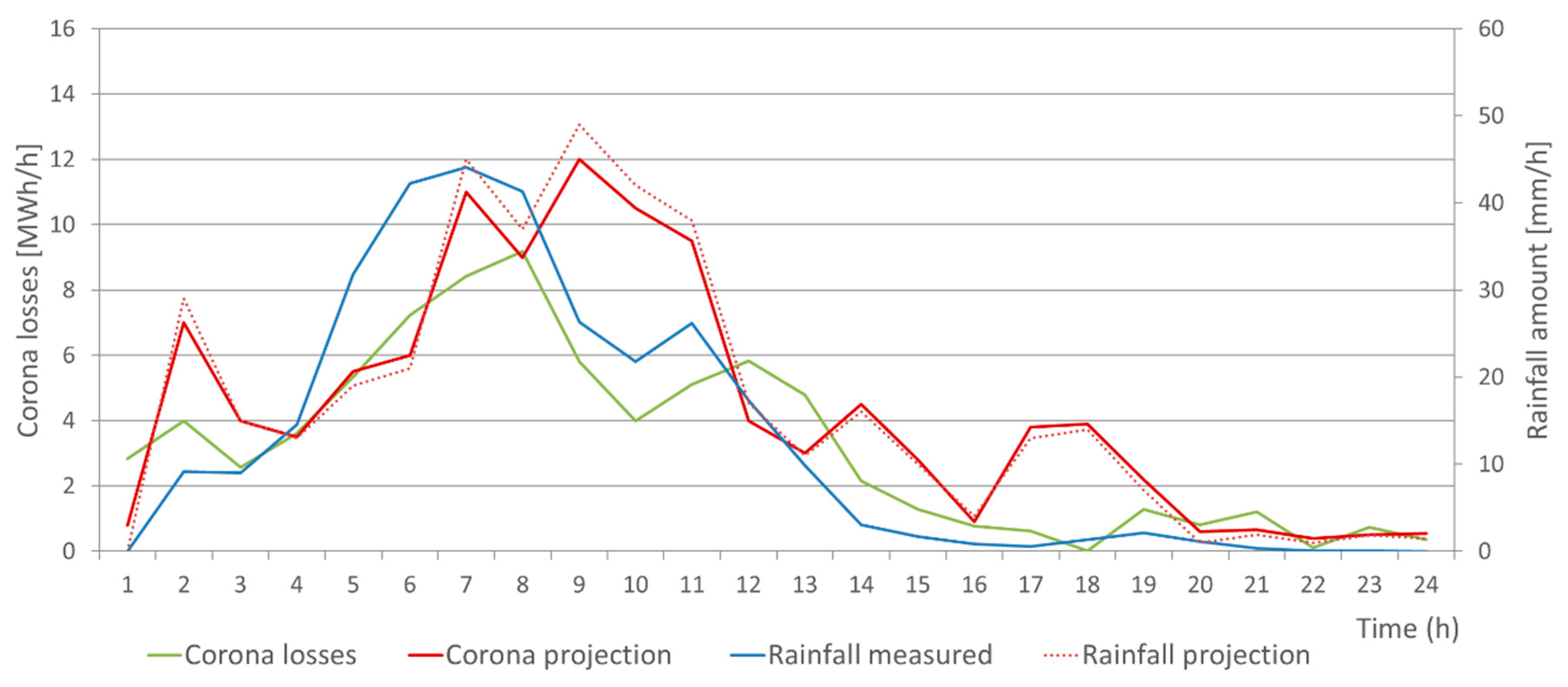
7.1. Forecast and Measurement of Rain

From the mentioned integrated weather prediction services (Section 5.4), the forecast for 20 May 2020 was selected. At the end of 18 May 2020, the weather forecast for each meteorological station on the corridor of each 400 OHL is taken and the amount of rain is then calculated for 20 May 2020. The calculation of weather forecasts is performed 72 h in advance, and is conducted every 6 h. This means that the first forecast that covers the selected period was performed on 18 May 2020.
Each meteorological station represents one segment of the 400 kV OHL and, based on the weather forecast, the total rainfall is calculated for each 400 kV OHL
To gain a better understanding of the correlation between the occurrence of corona losses and the amount of rain per OHL, Figure 19 shows the total amount of measured rain for each 400 kV OHL for 20 May 2020. To better understand the influence of precipitation on corona losses, it is necessary to know the exact amount of precipitation that is forecasted, and that is measured at each meteorological station.

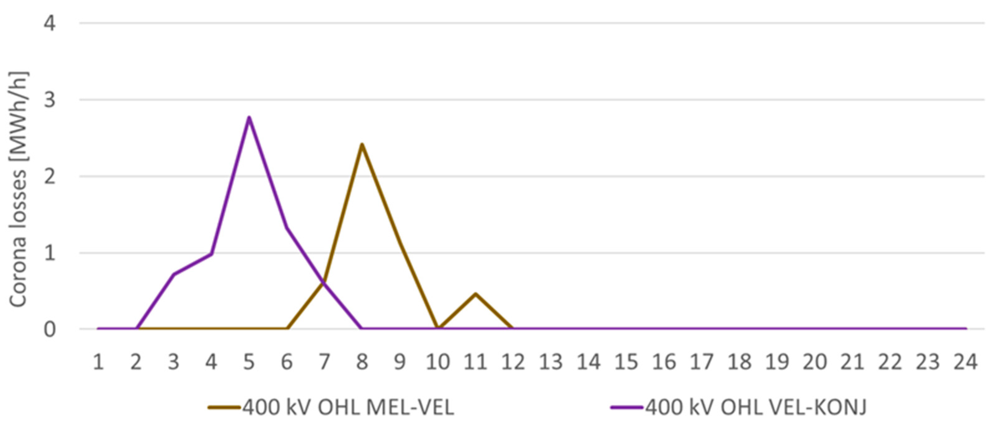
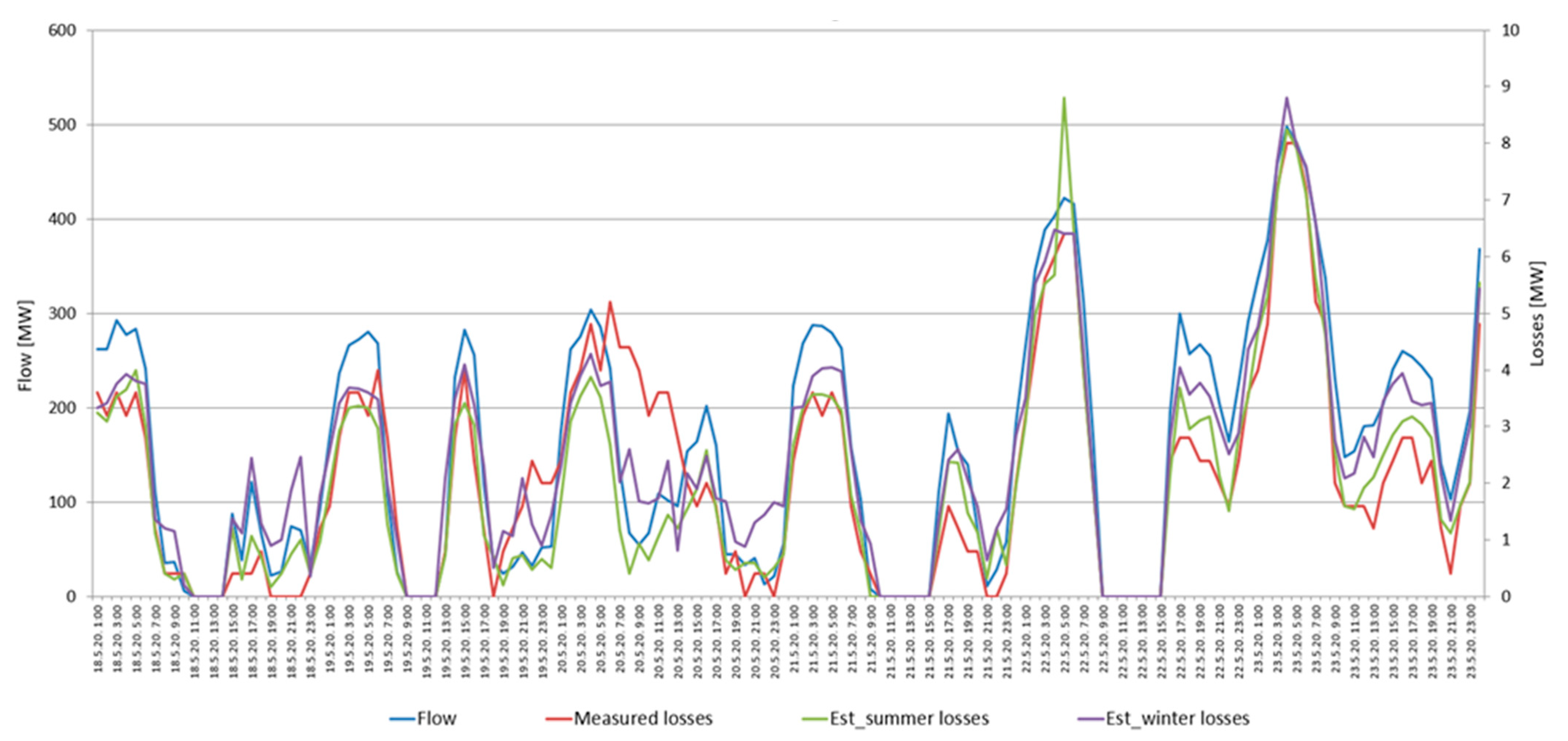
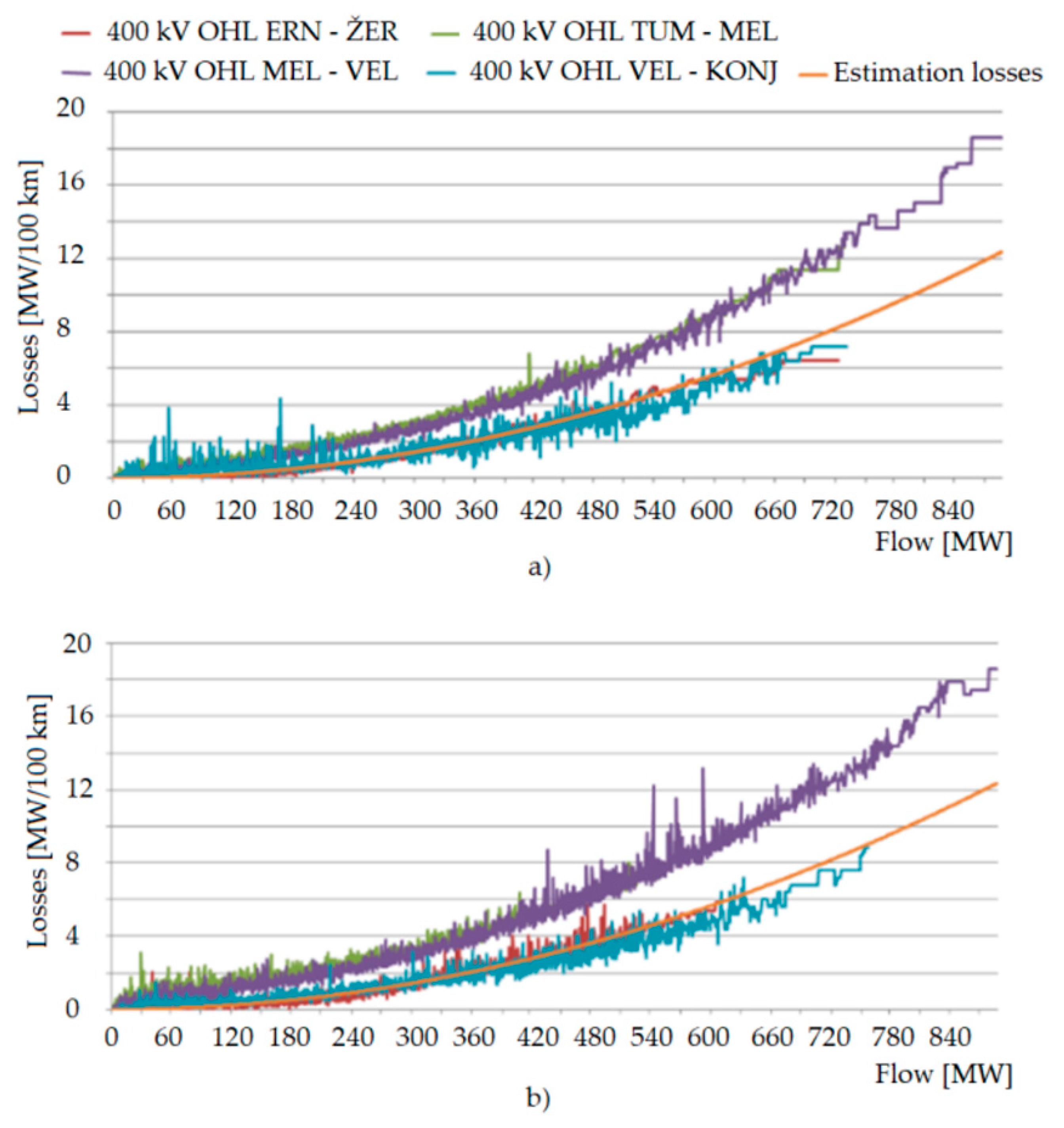
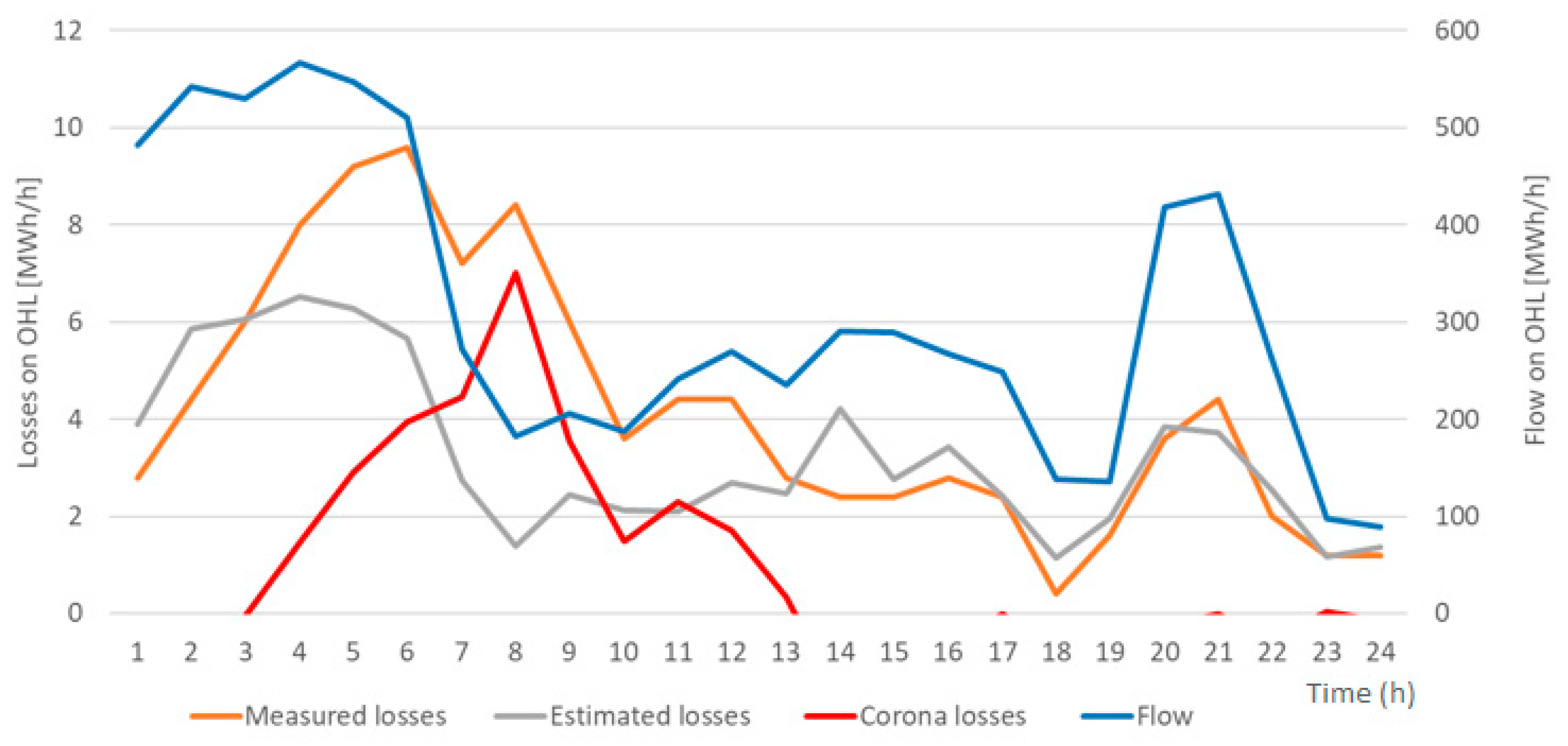
7.2. Prediction of Losses and Measurement on 400 kV

The prediction of losses is performed on a day-ahead basis in accordance with planned consumption, planned production and planned exchange. In this process, there are two dominant factors that currently affect the estimation of losses: (i) unscheduled power flow caused by unplanned production from renewable energy sources and (ii) cross-border flows and the influence of changing weather conditions. Uncertainty stemming from renewable energy production and cross-border flow has a lower influence on losses. On the other hand, the influence of the weather is much more influential, and changes in losses caused by it can be tracked efficiently, which is demonstrated by the proposed loss assessment model. Based on rainfall projections that were taken from the installed meteorological stations for each 400 kV OHL, corona projection is calculated as a function of the angle of the differential current from historical achievements and is presented as a red line in Figure 20. In the same figure, the total rainfall projection from the installed meteorological stations is presented as a dotted red line. The difference between the projection of the corona and rainfall can be explained as a result of the nature of the appearance of corona in the rain. When the maximum value of the corona is reached, an additional increase in the amount of rain does not lead to additional corona losses.
The prerequisite for loss projection calculation is the forecasting of weather conditions, mainly temperature and precipitation, for each region and geographical segment of the OHL corridor. After receiving the forecast data and the amount of precipitation for each meteorological station, analysis is performed to estimate the total amount of precipitation for each 400 kV OHL on an hourly basis for the selected day, 20 May 2020. Based on the total amount of precipitation for each 400 kV OHL, the regression method is conducted based on historically measured loss data, and for each 400 kV OHL, the estimation of corona is performed. In Figure 20, the estimation of the corona losses for the observed 400 kV OHL and comparison of the measured corona is presented. The difference in some hours is a direct consequence of differences between the forecasted and measured rainfall for 20 May 2020.

7.3. Comparing Losses with Weather Measurments

As was mentioned in Section 7.1, at each meteorological station in the corridor of each 400 kV OHL, a forecast is taken and compared with the measured amount of rain for a selected day of 20 May 2020. Based on this, a weather forecast for each 400 kV OHL was made.
From PMU measurements, it can be concluded that the level of corona losses that occurs on the selected day is significant, and can be presented as a difference between the measured total losses and the calculated ohmic losses. In Figure 21, the blue line represents the power flow for the observed 400 kV OHL, and correspondingly, the gray line represents the estimated losses. The orange line represents the measured losses throughout the day, and when the orange line is above the gray line, it can be concluded that there are additional losses compared to the estimated losses. The difference that occurs in the process of forecasting losses and especially corona losses is due to the uncertainty of weather forecasts. There is also uncertainty associated with measurements and the synchronization of all measurements, which has a significantly smaller influence.

8. Applicability of Proposed Loses Assessment Model and Results

In the process of the day-ahead loss planning, several analyses are conducted with the focus of establishing reasons for the deviation of measured losses from the planned losses. It can be observed that two dominant reasons for the deviation from planning losses are present. The most significant reason is unplanned power flows, and the second reason is the impact of weather conditions. The conducted analyses show that most of the losses due to bad weather occur on 400 kV OHL because of the occurrence of corona and leakage losses. Initial attempts at determining corona losses used the approach of processing statistical historically measured data separately for each 400 kV transmission line to determine the levels of losses for each transmission line. All performed analyses utilized the measurement data from electricity meters and SCADA systems. Although both systems represent important systems in the transmission network’s operation, there are certain shortcomings and limitations in the process of determining the losses on an hourly basis. Therefore, further research on the availability of measured quantities was started, and measurements from PMU devices were selected for additional measurements. The research presented in this paper has successfully shown that it is possible to use the measured values from PMU for a more detailed assessment of losses on 400 kV lines. The calculated values in this way are verified with measurements from other sources and are used for the purposes of determining losses at 400 kV.
The analysis showed that there are certain challenges in the collection of measurement data and their application in current and future business processes. It was noticed that at lower power flows, there is a larger error between the PMU measurement and the electricity meter measurements. The conducted analysis of the collected data showed that there is a higher scattering for the electricity meters, and the main cause for this was a large constant voltage (400 kW) and unsynchronized measurements. Currently, the procedure of planning and procuring losses is based on market principles and the time interval for trading is 1 h. In the near future, it is expected that the 15 min time interval for trading will be accepted, and the procurement of losses will be carried out on a 15 min time interval. In that case, the forecasting of losses will be more challenging due to the higher sensitivity to changing weather conditions and the higher frequency of measurement intervals.
Considering the mentioned challenges, the proposed assessment model for the determination of losses can improve the existing process of planning and procuring losses. The main advantage of the proposed procedure is the high level of possible integration into existing systems and the verification of existing billing measurements alongside the potential to reduce the costs in the loss procurement process caused by differences in predictions. The monitored and recorded conditions of the 400 kV transmission network and the measured losses for each transmission line are used in the creation of plans for the daily operation and development of the more efficient transmission network day-ahead planning.

9. Conclusions

The presented model for monitoring losses on 400 kV transmission lines represents an improvement to the process of determining Joule and corona losses on high-voltage transmission lines. From the available measurements and available input data, the prediction of losses can be made for each OHL considering predicted power flows. Using a similar methodology, the prediction of corona losses is performed based on weather forecasts. As already mentioned, the existing metering systems had certain limitations in the process of determining losses based on metering data, and so the use of metering data from PMU devices on 400 kV OHL was evaluated. In the first step, it was necessary to examine the possibilities of obtaining PMU data. A comparison of the measurement data for all operating conditions was made, and the analysis concluded that the measurements largely coincided with the measurements from the existing systems. By using Croatian TSO proprietary meteorological stations installed throughout the transmission network, it was possible to monitor weather conditions and obtain weather forecasts for each 400 OHL. This meteorological system was used as a source of historical weather data and as a forecasting tool for day-ahead plans. Combining the PMU data and weather conditions data led to the idea and realization of the model for the online assessment and forecasting of losses on the 400 kV network. With the developed model, it is possible to directly determine the total losses and additional losses caused by changes in weather and loading conditions. The results of the loss assessment model have significant importance, and can be used for the purpose of planning and procuring losses, leading to reduced costs of intraday market trading. Furthermore, the ability to manage electricity losses in the transmission system has practical significance, since they are an important technical and economic indicator of transmission system management, i.e., the lower the losses, the better the efficiency of transmission lines and the transmission network, and the proposed model contributes to this goal.

Author Contributions

Conceptualization, I.P. and N.H.; Data curation, I.P.; Investigation, I.P.; Methodology, I.P. and I.I.; Resources, D.B.; Software, D.B.; Validation, I.I.; Visualization, N.H.; Writing—original draft, I.P. and N.H.; Writing—review & editing, N.H. All authors have read and agreed to the published version of the manuscript.

Funding

This research received no external funding.

Institutional Review Board Statement

Not applicable.

Informed Consent Statement

Not applicable.

Acknowledgments

This work has been supported in part by H2020 project CROSSBOW (Grant 773430) and in part by European Structural and Investment Funds under project Konpro 2 (Razvoj nove generacije uređaja numeričke zaštite), grant KK.01.2.1.01.0096. This document has been produced with the financial assistance of the EU. The contents of this document are the sole responsibility of the authors and can under no circumstances be regarded as reflecting the position of the EU.

Conflicts of Interest

The authors declare no conflict of interest.

References

  1. 2nd CEER Report on Power Losses, Council of European Energy Regulators asbl, Cours Saint-Michel 30a, Box F–1040 Brussels, Belgium. 2020. Available online: https://www.ceer.eu/report-on-power-losses1# (accessed on 2 September 2021).
  2. Sivanagaraju, S. Electric Power Transmission and Distribution; Pearson Education India: Andhra Pradesh, India, 2008. [Google Scholar]
  3. Hu, J.; Harmsen, R.; Crijns-Graus, W. Developing a Method to Account for Avoided Grid Losses from Decentralized Generation: The EU Case. In Proceedings of the 4th International Conference on Power and Energy Systems Engineering, CPESE 2017, Berlin, Germany, 25–29 September 2017; pp. 25–29. [Google Scholar]
  4. Simões, P.F.M.; Souza, R.C.; Calili, R.F.; Pessanha, J.F.M. Analysis and short-term predictions of non-technical loss of electric power based on mixed effects models. Socio Econ. Plan. Sci. 2020, 71, 100804. [Google Scholar] [CrossRef]
  5. Pavičić, I.; Ivanković, I.; Šturlić, I.; Avramović, B.; Mance, M. Praćenje Gubitaka za Vodove Prijenosne Mreže, CIGRE 13. Simpozij o Sustavu Vođenja EES-a, November 2018. Available online: http://windlips.com/wp-content/uploads/2019/04/Pra%C4%87enje-gubitaka-za-vodove-prijenosne-mre%C5%BEe.pdf (accessed on 2 September 2021).
  6. Kolev, V.G.; Sulakov, S.I. The weather impact on the overhead line losses. In Proceedings of the 2017 15th International Conference on Electrical Machines, Drives and Power Systems (ELMA), Sofia, Bulgaria, 1–3 June 2017; pp. 119–123. [Google Scholar] [CrossRef]
  7. Tuttelberg, K.; Kilter, J. Real-time estimation of transmission losses from PMU measurements. 2015 IEEE Eindh. PowerTech 2015, 1–5. [Google Scholar] [CrossRef]
  8. Ghosh, S.; Ahmed, N.; Banerjee, S. Impact of Weather(Fog) on Corona Loss and Its Geographical Variation within Eastern Region. In Proceedings of the 2018 20th National Power Systems Conference (NPSC), Tiruchirappalli, India, 14–16 December 2018; pp. 1–6. [Google Scholar] [CrossRef]
  9. Clade, J.J.; Gary, C.H.; Lefevre, C.A. Calculation of Corona Losses beyond the Critical Gradient in Alternating Voltage. IEEE Trans. PAS 1969, 88, 695–703. [Google Scholar] [CrossRef]
  10. Pavičić, I.; Ivanković, I.; Župan, A.; Rubeša, R.; Rekić, M. Advanced Prediction of Technical Losses on Transmission Lines in Real Time. In Proceedings of the 2019 2nd International Colloquium on Smart Grid Metrology (SMAGRIMET), Split, Croatia, 9–12 April 2019. [Google Scholar]
  11. Tuttelberg, K.; Kilter, J. Estimation of transmission loss components from phasor measurements. Electr. Power Energy Syst. 2018, 98, 62–71. [Google Scholar] [CrossRef]
  12. Dasgupta, K.; Soman, S.A. Estimation of Zero Sequence Parameters of Mutually Coupled Transmission Lines from Synchrophasor Measurements. IET Gener. Transm. Distrib. 2017, 11, 3539–3547. [Google Scholar] [CrossRef]
  13. Ombua, A.; Labane, H.A. High voltage lines: Energy losses in insulators. Int. J. Eng. Sci. 2017, 6, 58–62. [Google Scholar]
  14. Deri, A.; Fodor, G. Infulence of geometric parameters on the corona loss of 220 kV and 400 kV overhead transmission lines. Tech. Univ. Bp. 1970, 14, 43–52. [Google Scholar]
  15. Khazaeia, J.; Fana, L.; Jiangb, W.; Manjure, D. Distributed Prony analysis for real-world PMU data. Electr. Power Syst. Res. 2016, 133, 113–120. [Google Scholar] [CrossRef]
  16. Saber, A.; Emam, A.; Elghazaly, H. Wide-Area Backup Protection Scheme for Transmission Lines Considering Cross-Country and Evolving Faults. IEEE Syst. J. 2018, 1–10. [Google Scholar] [CrossRef]
  17. Ivankovic, I.; Kuzle, I.; Holjevac, N. Multifunctional WAMPAC system concept for out-of-step protection based on synchrophasor measurements. Int. J. Electr. Power Energy Syst. 2017, 87, 77–88. [Google Scholar] [CrossRef]
  18. Ivankovic, I.; Rubesa, R.; Kuzle, I. Modeling 400 kV transmission grid with system protection and disturbance analysis. In Proceedings of the 2016 IEEE International Energy Conference (ENERGYCON), Leuven, Belgium, 4–8 April 2016; pp. 1–7. [Google Scholar]
  19. Mallikarjuna, B.; Chatterjee, D.; Reddy, M.J.B.; Mohanta, D.K. Real-Time Wide-Area Disturbance Monitoring and Protection Methodology for EHV Transmission lines. NAE Lett. 2018, 3, 87–106. [Google Scholar] [CrossRef]
  20. Naglic, M.; Popov, M.; Meijden, M.A.M.M.; Terzija, V. Synchro-measurement Application Development Framework: An IEEE Standard C37.118.2-2011 Supported MATLAB Library. IEEE Trans. Instrum. Meas. 2018, 67, 1804–1814. [Google Scholar] [CrossRef]
  21. Lavenius, J.; Vanfretti, L. PMU-Based Estimation of Synchronous Machines’ Unknown Inputs Using a Nonlinear Extended Recursive Three-Step Smoother. IEEE Access 2018, 1–14. [Google Scholar] [CrossRef]
  22. Vaiman, M.; Quint, R.; Silverstein, A.; Papic, M.; Kosterev, D.; Leitschuh, N.; Faris, A.; Yang, S.; Blevins, B.; Rajagopalan, S.; et al. Using Synchrophasors to Improve Bulk Power System Reliability in North America. In Proceedings of the 2018 IEEE PES General Meeting, At Portland, OR, USA, 5–10 August 2018; pp. 1–5. [Google Scholar]
  23. Ivanković, I.; Peharda, D.; Novosel, D.; Žubrinić-Kostović, K.; Kekelj, A. Smart grid substation equipment maintenance management functionality based on control center SCADA data. J. Energy 2018, 67, 30–35. [Google Scholar]
  24. Ivanković, I.; Jaman, N. Using Data from SCADA for Centralized Transformer Monitoring Applications. In Proceedings of the 4th International Colloquium “Transformer Research and Asset Management”, Pula, Croatia, 10–12 May 2017. [Google Scholar]
  25. Preglej, S.; Dujmović, A.; Dereani, D. Sustavi za Nadzor Kvalitete Električne Energije na Točkama Predaje Velikim Industrijskim Potrošačima. CIRED. 2008. Available online: http://www.ho-cired.hr/wp-content/uploads/2013/06/SO2-07.pdf (accessed on 2 September 2021).
Figure 1. Typical categorization of power losses (adopted from [1], 2020, CEER).
Energies 14 05562 g001
Figure 2. Components of T&D losses and their shares in total energy losses (adopted from [3], 2017, CPESE).
Energies 14 05562 g002
Figure 3. General classification of losses in the transmission system.
Energies 14 05562 g003
Figure 4. Line differential protection functions based on synchrophasor data: (a) operating characteristic for line differential protection; (b) conditions for triggering the functions with the differential and restrained current ratio.
Energies 14 05562 g004
Figure 5. Vectors of the current and voltage phasors on OHLs.
Energies 14 05562 g005
Figure 6. Differential current angles of the Melina-Velebit and Velebit-Konjsko 400 kV lines during a period of 24 h on 20 May 2020.
Energies 14 05562 g006
Figure 7. Estimated values of corona losses for 400 kV lines and correlations with the differential current angle during a period of 24 h on 20 May 2020.
Energies 14 05562 g007
Figure 8. Block scheme of Croatian 400 kV transmission network with the marked PMU measurements.
Energies 14 05562 g008
Figure 9. Flow chart of the model for calculating on-line and prediction of losses.
Energies 14 05562 g009
Figure 10. Croatian transmission grid.
Energies 14 05562 g010
Figure 11. Main technical characteristics of 400 kV lines.
Energies 14 05562 g011
Figure 12. Total losses (kWh) on an hourly basis for the observed 400 kV transmission grid (heat map) for a 30-day period and for each hour of the day.
Energies 14 05562 g012
Figure 13. Actual load flow, measured losses, and estimation of losses on an hourly basis for the observed 400 kV OHL.
Energies 14 05562 g013
Figure 14. Comparison of power flow measurements and difference between ADVANC and PMU measurements in SS Velebit and SS Konjsko.
Energies 14 05562 g014
Figure 15. Comparison of total losses on the 400 kV OHL Velebit-Konjsko from ADVANC and PMU measurements.
Energies 14 05562 g015
Figure 16. Meteorological stations in Croatia and the configuration of the meteorological system.
Energies 14 05562 g016
Figure 17. Losses on 400 kV OHLs for periods based on historical measurements with ohm losses expressed with orange line for: (a) the winter period; and (b) the summer period.
Energies 14 05562 g017
Figure 18. Losses on a 400 kV transmission grid showing the occurrence of corona losses for a daily period for 20 May 2020.
Energies 14 05562 g018
Figure 19. Measured rainfall for each 400 kV OHL on the selected day—20 May 2020.
Energies 14 05562 g019
Figure 20. Comparison of the corona prediction values and measured corona values for the observed 400 kV OHL on 20 May 2020.
Energies 14 05562 g020
Figure 21. Measured losses and classification of losses for the 400 kV OHL on the chosen day, 20 May 2020.
Energies 14 05562 g021
Table 1. Corona losses due the different weather conditions (adopted from [5], 2018, HRO CIGRE).
Weather Condition DescriptionCorona Losses (kW/km)
220 kV400 kV
12 Conductors per Phase3 Conductors per Phase
1Dry0.20.660.17
2Rain-28.17.6
3Frost on conductor-34.513.5
Table 2. Leakage losses due the different weather conditions (adopted from [13], 2017, Int. J. Eng. Sci.).
Weather ConditionLosses on Insulators (W/insul.)
220 kV400 kV
1Dry0.10.3
2Light fog0.150.5
3Snow below 0 °C0.250.8
4Heavy rain13.2
5Heavy continuous rain1.13.6
6Storm1.54.9
7Rain with heavy snow2.27.1
Publisher’s Note: MDPI stays neutral with regard to jurisdictional claims in published maps and institutional affiliations.

