Obtaining Robust Performance of a Current fed Voltage Source Inverter for Virtual Inertia Response in a Low Short Circuit Ratio Condition

Abstract

Low inertia levels are typical in island power systems due to the relatively small rotational generation. Displacing rotational generation units with static inertia-less PV power results in a significant increase in the frequency volatility. Virtual inertia provided by inverter-storage systems can resolve this issue. However, a low short circuit ratio (SCR) at the point of common coupling together with a fast phase locked loop (PLL) will compromise the response performance of the system. To address this issue, a robust PI controller (RPI) for the inner current-loop of a current fed grid-connected inverter is proposed. The PLL disturbance and grid impedance are incorporated into a single model and recast to a generalized representation of the system, thereby allowing easy tuning of the RPI by the mixed sensitivity H_∞ method. The performance of the RPI is compared with that of a PI controller (PI) tuned by the regular loop-shaping method. The results show that when the SCR is above 10, the performance of both controllers is equivalent. However, lowering of the SCR compromises the performance of the system with PI and it becomes underdamped at SCR < 2. On the contrary, the system with the RPI is capable of maintaining the nominal performance throughout the same SCR decrease.

1. Introduction

Low inertia island grids have intricate frequency regulation challenges when inverter-based generation such as Photovoltaic systems (PV) are integrated. However, attractive financial incentives are driving the displacement of diesel-based generation by PV. The successful large-scale integration of PV into existing grids necessitates solutions aimed at mitigating the resulting increase in frequency volatility, thereby preventing PV curtailment, especially in low inertia grids. Field measurements on the island grids of Bornholm and Bonaire have shown that the time rate of change of frequency (ROCOF) can vary from 4 Hz/s to up to as high as 10 Hz/s [1,2]. This is in contrast to the ROCOF levels of 100 mHz/s to 1 Hz/s in the interconnected European system where inertia levels are sufficient [3]. ROCOF levels exceeding 2 Hz/s are undesirable for grid stability due to factors such as pole slipping in synchronous generators, stable connection of inverter-based generation where Phase Locked Loop (PLL) systems are employed, and inadequate operation of under frequency load shedding protection [4,5]. Frequency response measures such as Virtual Inertia Response (VIR) provided through grid-connected inverters with chemical battery energy storage systems (BESS) have proven to be a technically viable solution to increasing the amount of available inertia in the grid and thereby improving the ROCOF. It has been demonstrated that BESS-based VIR is capable of improving the zonal inertia in the South Australia grid where the penetration level of inverter-based generation can reach 60% of the demand [6]. The obtained improvement in the ROCOF level resulted in a more stable interconnection (which is constrained by a 3 Hz/s ROCOF limit) with larger inertia segments of nearby existing grids. Other field experience in island grids have also shown that the capability of inverter-based storage systems to exchange power with the grid within 58 to 200 milliseconds after a frequency event have decreased the frequency volatility, thereby preventing power outages [7,8]. However, due to relatively large occurring ROCOFs in low inertia island grids, successful VIR implementation requires that the PLL necessary for measuring the frequency be of sufficient bandwidth (BW). Inadequate BW of the PLL may result in inaccurate frequency measurements [5] and, therefore, inaccurate calculation of the ROCOF. The results in [2] have shown that a ROCOF in the range of 10 Hz/s require that the PLL bandwidth be at least a decade greater than normally would be the case. The high BW requirement of the PLL unfortunately imposes another challenge for successful implementation of the inverter-based VIR. A low short circuit ratio (SCR) at the Point of Common Coupling (PCC) of the inverter and grid together with the high BW PLL will compromise the performance and stability of the inverter-storage system. Low SCR, a weak grid condition, is typical in island grids due to factors such as the radial structure of the grid and long sparse transmission lines [9]. A high BW PLL renders the behavior of the inverter closed-loop output impedance into that of a predominantly negative resistor at low frequencies. This behavior may cause instability upon interaction with a large enough grid impedance (low SCR) [10]. Power electronic converter stability issues due to interaction of the input impedance of the converter (the downstream impedance) and that of the upstream impedance (e.g., output filter, load or line) have long been an issue, resulting in Middlebrook’s stability criteria for input filter design published in 1976 [11]. Since then, numerous studies have investigated the effect of the upstream impedance on the dynamics of power electronic converters and have presented solutions ranging from active damping to tuning methods for the inner-loop current controller. The work in [12] proposed an active damping scheme whereby the capacitor current of the LCL filter is used in a positive feedback proportional-integral (PI) control loop to virtually extend the positive equivalent resistance range, thereby obtaining robustness of the inverter against grid impedance variations. Essentially, this method prevents degradation of the phase margin (PM) due to grid impedance variations. The PLL impact on the inverter dynamics was, however, excluded. In [13], an adaptive block is added to the feedback loop of the PLL and a cancellation gain based on an estimation of the grid impedance is calculated to eliminate the coupling of the PLL and grid impedance. It is, however, unclear to what extent the estimation error and high BW PLL may compromise the method. Research has also given attention to the idea that an inner-loop current controller can be successfully designed to provide robustness of the inverter against upstream impedance interaction as demonstrated in [14]. Since then, others have followed and successfully designed various types of controllers. In [15], a filtered error tracking controller is adopted and implemented in the αβ-frame, which eliminated the need for a PLL. These type of controllers are fundamentally designed to tightly track the reference. It was shown that once a set of smooth current references were provided to the controller, the inverter maintained nominal performance during a sudden increase of the grid impedance. Similarly, other types of controllers implemented in the αβ-frame including a robustly tuned Proportional Resonant (PR) controller, and a combination of PR and a lead compensator are proposed in [16,17]. While these solutions in the αβ-frame may be promising, VIR implementation requires determination of the grid voltage angle, and the synchronous reference frame PLL (SRF-PLL) is widely adopted in three phase inverters for this purpose [18]. Robust controller design methods such as H_∞ optimization have also been successfully applied to obtain robust controllers [19,20,21]. The obtained controllers were, however, of higher order compared to the simple structure of a PI controller, and the coupling between the PLL and the grid impedance was not taken into account. In [22], it was shown that the regular PI controller can be designed with adequate stability margins to withstand increases in the grid impedance and, as demonstrated in [23], even against the PLL-grid impedance coupling.

Based on the foregoing summary, the aim of this work is then to propose a solution that would allow successful VIR implementation in island grids where weak grid conditions of both low inertia and low SCR coexist and, as a result, degrade the performance of the inverter system. This work builds on the idea that the inner-loop current controller can be tuned to provide inverter robustness. Unlike previous research presented, this work takes a different approach and proposes adopting the H_∞ optimization method such that the regular and simple structure of the PI controller is maintained and tuned to achieve inverter robustness against PLL-grid impedance coupling. To achieve this, a validated small signal model of a current fed inverter is recast into a generalized representation and the PLL-grid impedance coupling is treated as a single multiplicative perturbation. The formulation of the PLL-grid impedance coupling into a single perturbation then allows for easy application of the mixed sensitivity H_∞ optimization method. It is shown that the H_∞ tuned PI controller is capable of providing inverter robustness against the coupling of a 50 Hz PLL and SCR < 3. The rest of this paper is organized as follows: in Section 2, a detailed switching model of a current fed inverter is built in MATLAB/Simulink (The MathWorks, Inc.: Natick, MA, USA) and validated with lab measurements. The transfer functions of the validated model are presented in Section 3 and verified through a frequency response comparison. In Section 4, a generalized representation of the inverter model together with the PLL-grid impedance coupling is developed. The performance of the obtained H_∞ PI controller in weak grid conditions is presented in Section 5, and finally, conclusions are formulated in Section 6.

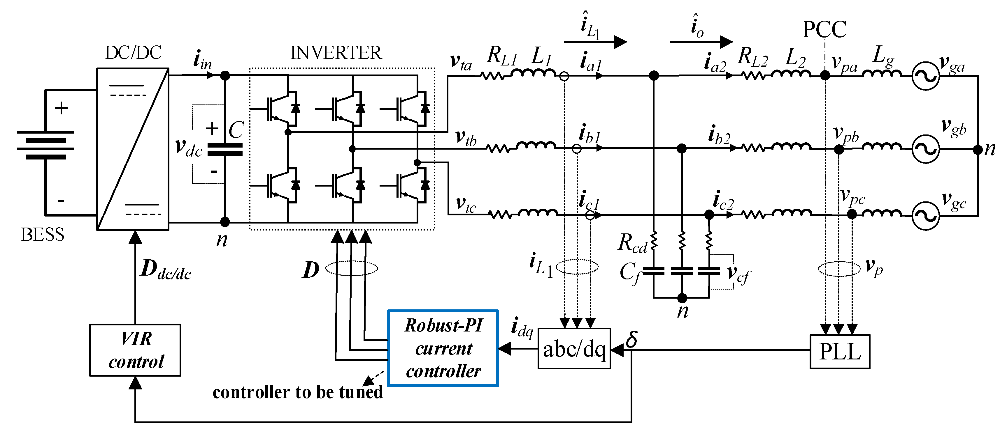
2. Modeling and Validation

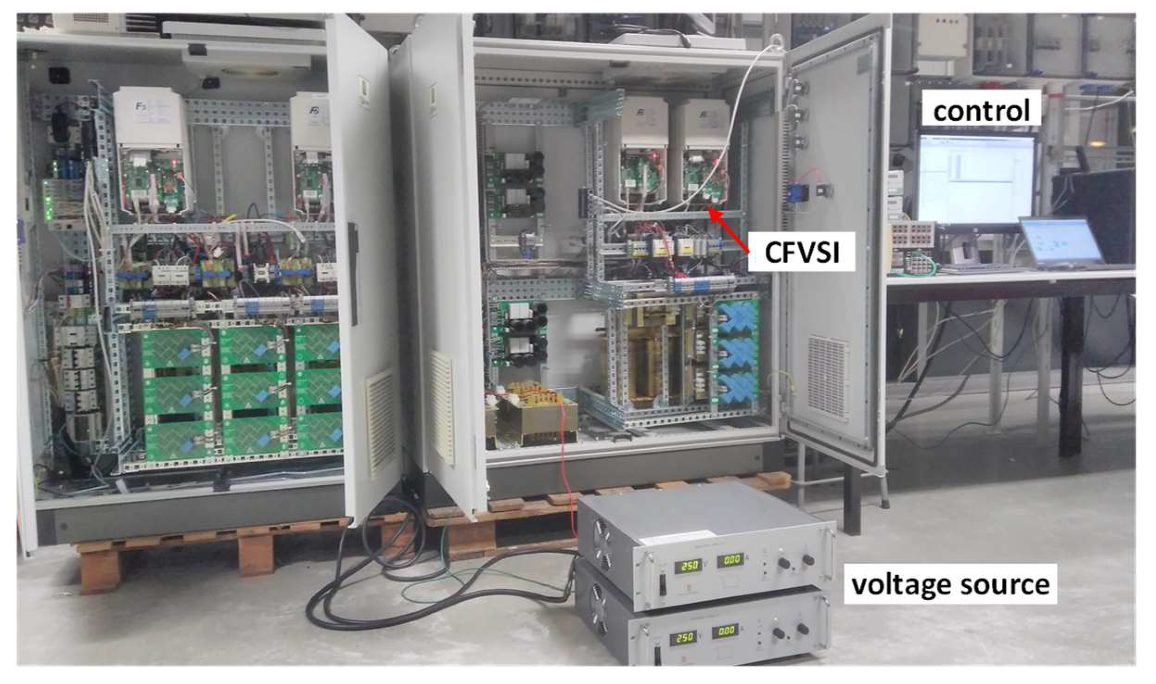
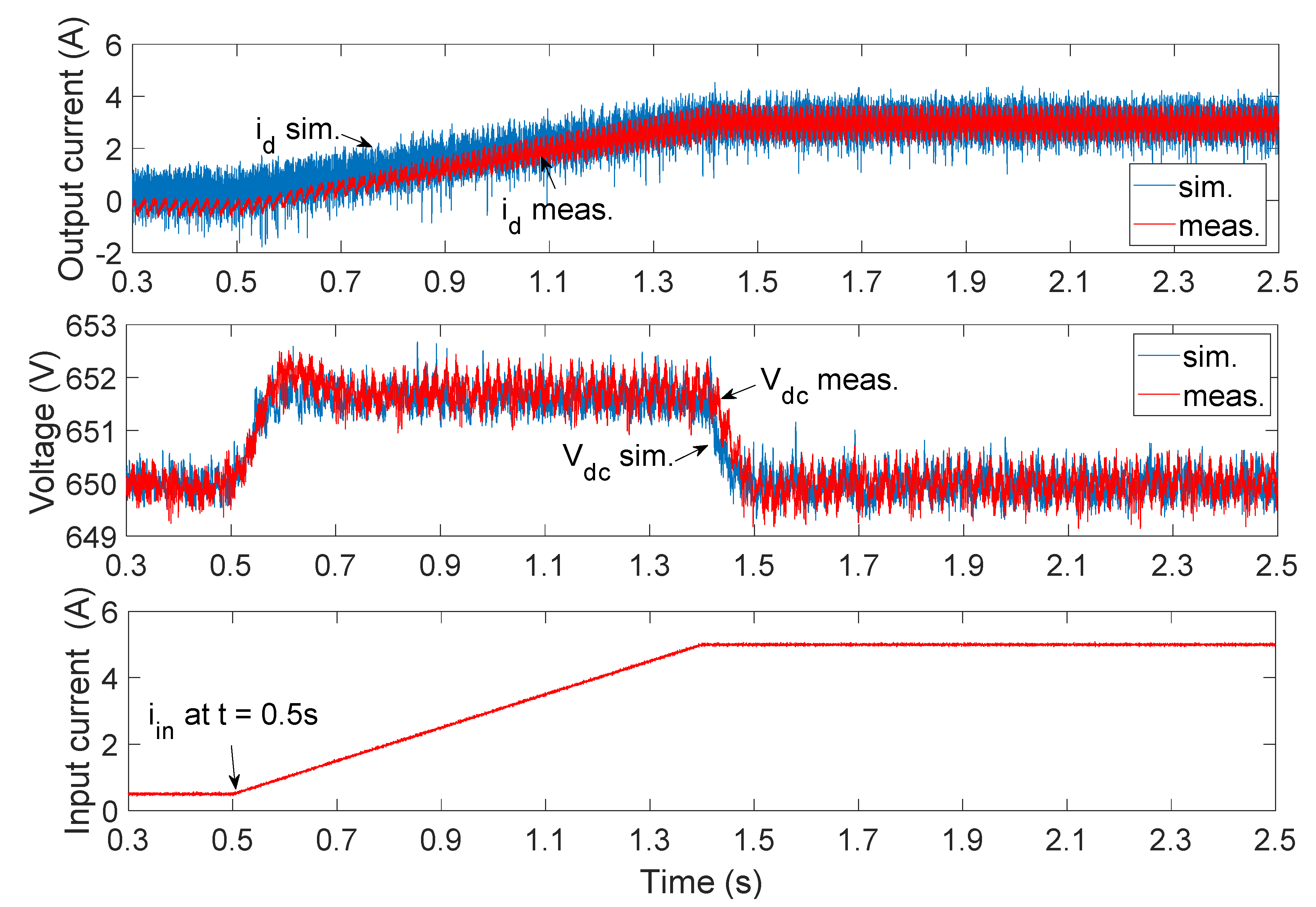
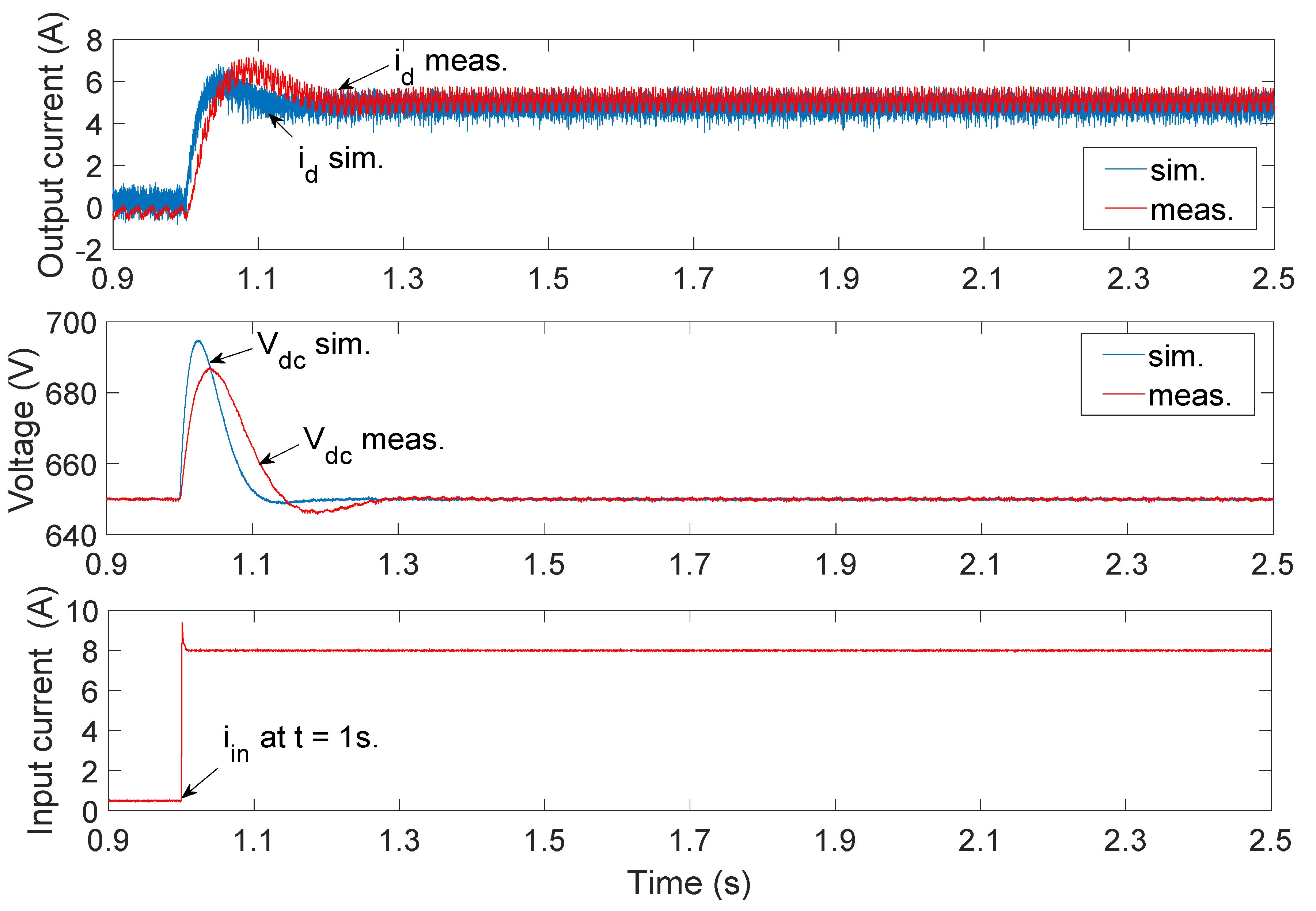
2.1. Validation of Detailed Switching Model

A current fed voltage source inverter (CFVSI) available in a lab is depicted in Figure 1 and the corresponding parameters are listed in

Table 1. CFVSI parameters.

Parameter	Value	Unit
Rated power	17	kVA
Rated voltage	400	V
DC link voltage	650–750	V
DC link capacitance C	0.75	$\mathrm{mF}$
Filter inductance L1; L2	22.3; 1.28	$\mathrm{mH}$
Filter resistance RL1; RL2	200	$\mathrm{m}\mathsf{\Omega }$
Filter capacitance Cf	8.8	$\mathsf{\mu }\mathrm{F}$
Switching frequency, fs	8–20	kHz
Fundamental frequency	50	$\mathrm{Hz}$

. The schematic diagram of the CFVSI is shown in Figure 2, which also depicts the situation where the CFVSI system is connected to a grid through the line impedance Z_g. In the virtual inertia scheme, a reference signal can be issued to the DC-DC converter, thereby extracting (or absorbing) the corrective power from the BESS and exchanging it through the CFVSI with the grid. The time rate of change of the reference signal varies with the ROCOF, which is calculated by the “VIR control block” based on the angle δ issued by the PLL, as shown in Figure 2.

The control analysis in time-domain was conducted through simulations with a detailed switching model of the CFVSI built in the software package MATLAB/Simulink. To validate the model, the aforementioned VIR scheme was emulated in the lab and the CFVSI dynamic response of the DC link voltage, grid currents, and voltages in both dq- and abc-domains were recorded. The measurements were sampled at the inverter switching frequency of 8 kHz, which is well above the 1.5 kHz resonant frequency of the inverter LCL filter [24]. The same scheme was simulated with the MATLAB/Simulink model, and the simulated results were compared to the experimental recordings. Figure 3, Figure 4 and Figure 5 show the measured and simulated responses of the DC link voltage of which the setpoint voltage was 650 V, and the d-component of the grid currents for the three current injections is as follows: 5 A at a rate of 5 A/s, 8 A instantaneously, and 10 A at 100 A/s.

Comparison of the simulated responses to the recordings show that the model is capable of representing the dynamics of the real system.

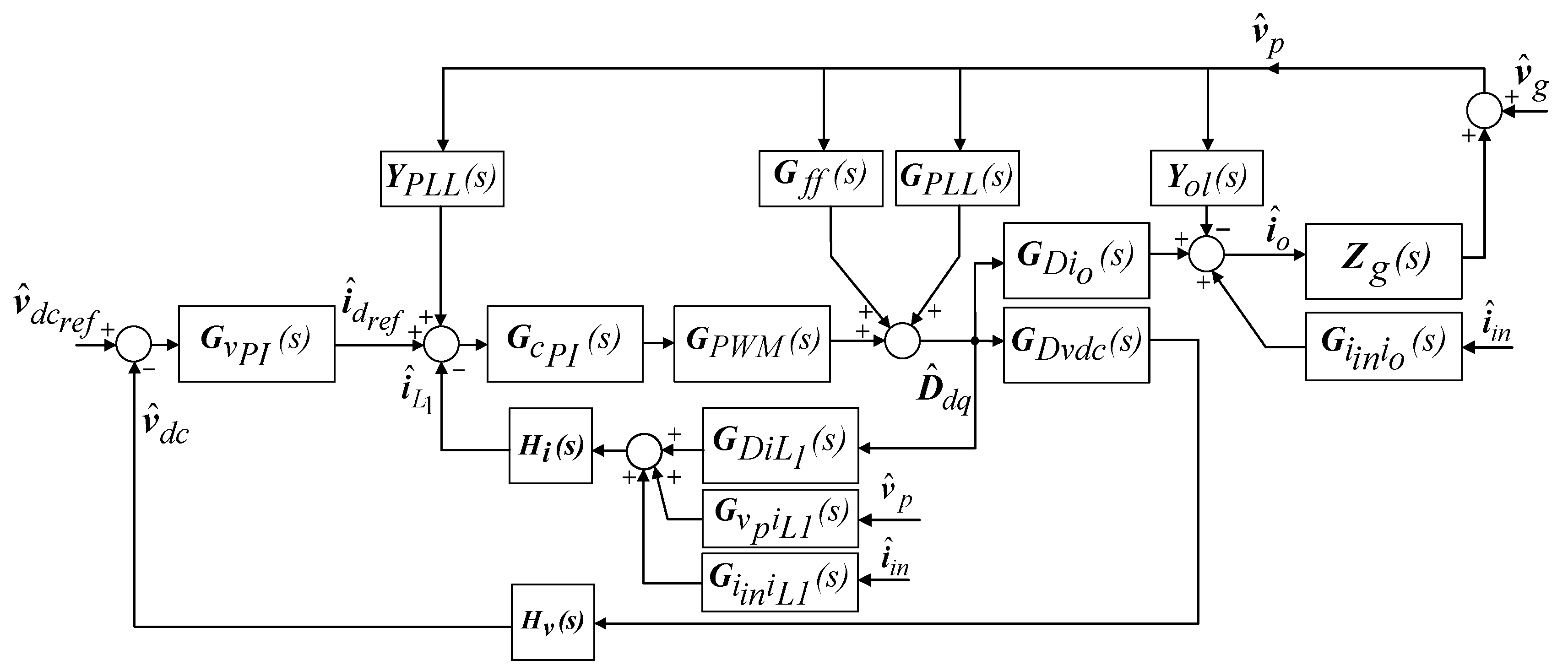
2.2. Small Signal Model of the CFVSI

Next, a linear small signal model of the CFVSI was derived using space phasor variables. The inductor currents i_L1 and i_o and capacitor voltages v_dc and v_cf, as depicted in Figure 2, were chosen as state variables of the system, with input and output variables defined, respectively, as: i_in, v_p, D; and v_dc, i_L1, i_o. Referring to Figure 2, the set of simultaneous differential equations describing the dynamics of the balanced three phase system could then be formulated in space phasor form to give Equation (1).

(1)

where the variables in brackets are averaged values.

After (1) is expanded (e.g.,$\frac{d〈\overrightarrow{i_{L_1}}〉}{dt}=\left(i_{L_{1d}}+j{i}_{L_{1q}}\right)e^{j\delta (t)}$), solved, and linearized, the variables can be decomposed into their dq-components. The obtained expression can then be written in the state-space form of (2). The obtained corresponding state-space matrices are given in Appendix A.

$$\left\{\begin{array}{l}s\mathit{X}(s)=\mathit{A}\mathit{X}(s)+\mathit{B}\mathit{U}(s)\\ \mathit{Y}(s)=\mathit{C}\mathit{X}(s)+\mathit{D}\mathit{U}(s)\end{array}\right.$$

(2)

The open-loop transfer functions in the s-domain can be found by applying the transfer function matrix in (3) to (2), as elaborated in [25].

$$\mathit{G}(s)=\frac{\mathit{Y}(s)}{\mathit{U}(s)}=\mathit{C}{\left(s\mathit{I}-\mathit{A}\right)}^{-1}\mathit{B}+\mathit{D}$$

(3)

where I is the identity matrix.

The obtained open-loop transfer functions are collected in G(s) and are given in Appendix A. The 2 by 2 transfer matrices relate the corresponding output to input vectors. With the open-loop transfer functions now available, the total system block diagram can be constructed, as shown in Figure 6. The block diagram includes the dynamics of the PLL and the grid impedance Z_g. The PLL transfer functions G_PLL and Y_PLL can be derived as elaborated in [26], and are given in Appendix A. The typical cascade control configuration contains an outer-loop voltage controller and an inner-loop current controller, denoted here, respectively, by ${\mathit{G}}_{{\mathit{v}}_{PI}}$ and ${\mathit{G}}_{c_{PI}}$. The DC link voltage is regulated by issuing the reference current ${\mathit{i}}_{d_{ref}}$ to ${\mathit{G}}_{c_{PI}}$, thereby transferring the input power to the grid. The two loops are isolated by making the inner-loop faster than the outer-loop, i.e., designing ${\mathit{G}}_{c_{PI}}$ to be at least a decade higher than ${\mathit{G}}_{{\mathit{v}}_{PI}}$ [27].

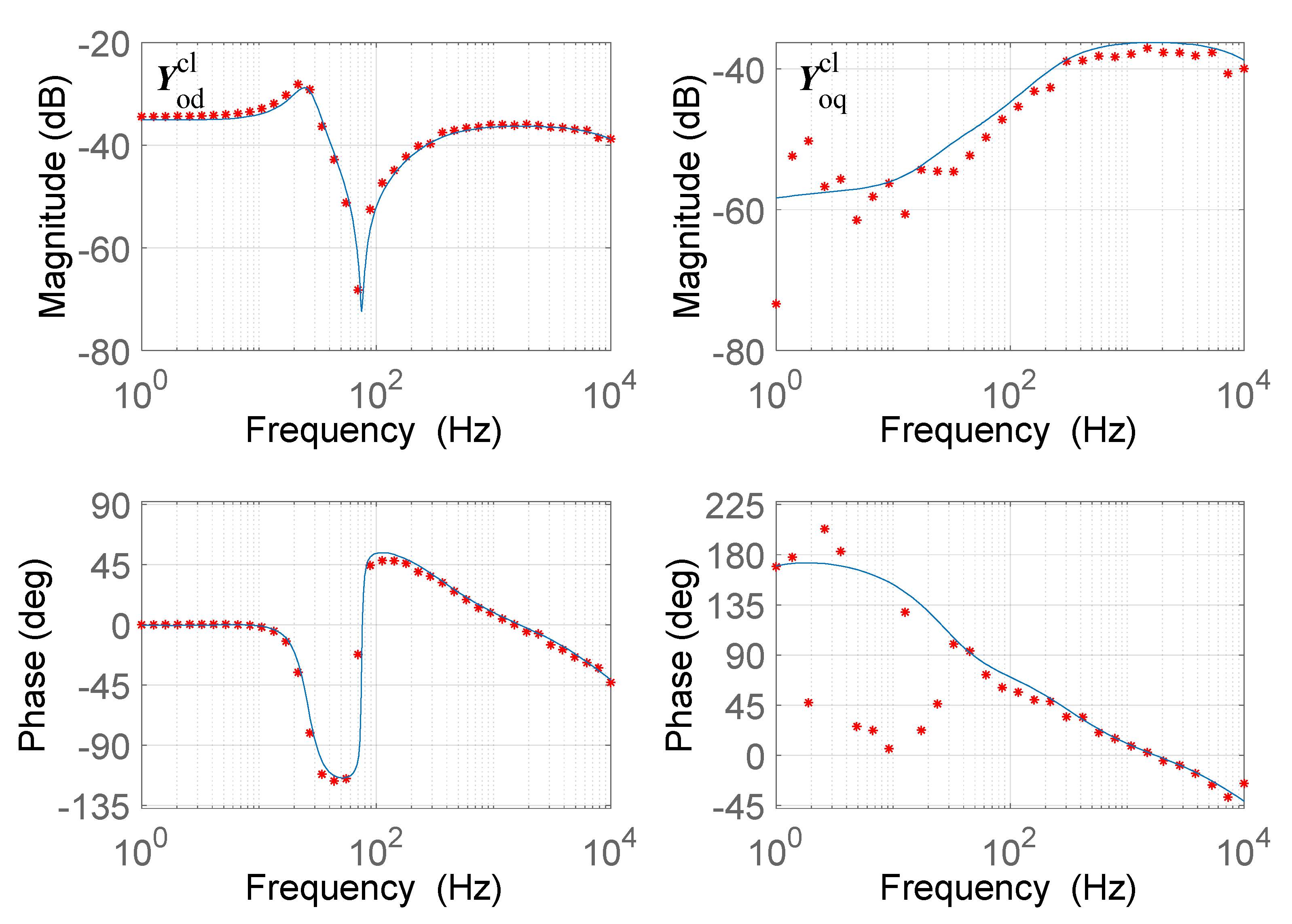
3. Transfer Functions Verification

In this section, the closed loop transfer functions of the detailed CFVSI are presented and verified. It should be pointed out that, in the simulations, the grid current is measured on the inverter side, as shown in Figure 2; however, to take the effect of both the PLL and grid inductance into account, the closed-loop transfer functions are derived based on the current ${\widehat{\mathit{i}}}_o$ entering Z_g. The closed-loop output admittance Y_ocl, i.e., the transfer function from ${\widehat{\mathit{v}}}_p$ to ${\widehat{\mathit{i}}}_o$ with both the inner current-loop and the outer voltage-loop closed, can be derived from the corresponding open-loop transfer functions. The open-loop transfer functions are obtained from the matrix G(s) and given by (4) and (5), with the dq sub-subscripts omitted for brevity.

$${\widehat{\mathit{i}}}_o={\mathit{G}}_{{\mathit{i}}_{in}{\mathit{i}}_o}{\widehat{\mathit{i}}}_{in}-{\mathit{Y}}_{ol}{\widehat{\mathit{v}}}_p+{\mathit{G}}_{\mathit{D}{\mathit{i}}_o}\widehat{\mathit{D}}$$

(4)

$${\widehat{\mathit{v}}}_{dc}={\mathit{G}}_{{\mathit{i}}_{in}{\mathit{v}}_{dc}}{\widehat{\mathit{i}}}_{in}+{\mathit{G}}_{{\mathit{v}}_p{\mathit{v}}_{dc}}{\widehat{\mathit{v}}}_p+{\mathit{G}}_{\mathit{D}{\mathit{v}}_{dc}}\widehat{\mathit{D}}$$

(5)

The closed-loop transfer functions for the inner current-loop are found by solving for the duty ratio $\widehat{\mathit{D}}$ and then substituting the obtained expression into (4) and (5). By inspection of Figure 6, the following expression for $\widehat{\mathit{D}}$, which includes the PLL dynamics, is obtained:

$$\begin{array}{l}\widehat{\mathit{D}}={\left(\mathit{I}+L_c\right)}^{-1}\left\{{\mathit{G}}_{PWM}{\mathit{G}}_{c_{P\mathit{I}}}{\widehat{\mathit{i}}}_{d_{ref}}-H_{\mathit{i}}{\mathit{G}}_{PWM}{\mathit{G}}_{c_{P\mathit{I}}}{\mathit{G}}_{{\mathit{i}}_{in}{\mathit{i}}_{L_1}}{\widehat{\mathit{i}}}_{in}\right.\\ \left.\left[\left({\mathit{G}}_{ff}+{\mathit{G}}_{PLL}\right)+{\mathit{G}}_{PWM}{\mathit{G}}_{c_{P\mathit{I}}}\left({\mathit{Y}}_{PLL}-H_{\mathit{i}}{\mathit{G}}_{{\mathit{v}}_p{\mathit{i}}_{L_1}}\right)\right]{\widehat{\mathit{v}}}_p\right\}\end{array}$$

(6)

With, $L_c=H_{\mathit{i}}{\mathit{G}}_{\mathit{D}{\mathit{i}}_{L_1}}{\mathit{G}}_{PWM}{\mathit{G}}_{c_{P\mathit{I}}}$.

The closed-loop dynamics including the outer voltage-loop are found by replacing ${\widehat{\mathit{i}}}_{d_{ref}}$ in (6) with the following expression obtained from Figure 6:

$${\widehat{\mathit{i}}}_{d_{ref}}=\left({\mathit{v}}_{d{c}_{ref}-H_{\mathit{v}}}{\widehat{\mathit{v}}}_{dc}\right){\mathit{G}}_{{\mathit{v}}_{P\mathit{I}}}$$

(7)

Substitution of the obtained $\widehat{\mathit{D}}$ into (5) yields the following expression for the closed-loop dynamics:

$${\widehat{\mathit{v}}}_{dc}={\mathit{G}}_{{\mathit{i}}_{in}{\mathit{v}}_{dc}}^{cl}{\widehat{\mathit{i}}}_{in}+{\mathit{G}}_{{\mathit{v}}_p{\mathit{v}}_{dc}}^{cl}{\widehat{\mathit{v}}}_p+{\mathit{G}}_{{\mathit{v}}_{d{c}_{ref}}{\mathit{v}}_{dc}}^{cl}{\widehat{\mathit{v}}}_{d{c}_{ref}}$$

(8)

$${\widehat{\mathit{i}}}_o={\mathit{G}}_{{\mathit{i}}_{in}{\mathit{i}}_o}^{\mathit{i}l}{\widehat{\mathit{i}}}_{in}-{\mathit{Y}}_o^{\mathit{i}l}{\widehat{\mathit{v}}}_p+{\mathit{G}}_{{\mathit{i}}_{d_{ref}}{\mathit{i}}_o}\left({\widehat{\mathit{v}}}_{d{c}_{ref}}-H_{\mathit{v}}{\widehat{\mathit{v}}}_{dc}\right){\mathit{G}}_{{\mathit{v}}_{P\mathit{I}}}$$

(9)

Finally, replacing ${\widehat{\mathit{v}}}_{dc}$ in (9) with (8) yields the total closed-loop dynamics of the output current, which is given by:

$${\widehat{\mathit{i}}}_o={\mathit{G}}_{{\mathit{i}}_{in}{\mathit{i}}_o}^{cl}{\widehat{\mathit{i}}}_{in}-{\mathit{Y}}_o^{cl}{\widehat{\mathit{v}}}_p+{\mathit{G}}_{{\mathit{v}}_{d{c}_{ref}}{\mathit{i}}_o}^{cl}{\widehat{\mathit{v}}}_{d{c}_{ref}}$$

(10)

The full expressions of the closed-loop transfer functions in (8) and (9) are given in Appendix A. The closed-loop output admittance of the inverter with both inner-and outer-loops closed is given by:

$$\frac{{\widehat{\mathit{i}}}_o}{{\widehat{\mathit{v}}}_p}={\mathit{Y}}_o^{cl}={\mathit{Y}}_o^{\mathit{i}l}+{\mathit{G}}_{{\mathit{i}}_{d_{ref}}{\mathit{i}}_o}{\mathit{G}}_{{\mathit{v}}_{P\mathit{I}}}{H}_{\mathit{v}}{\mathit{G}}_{{\mathit{v}}_p{\mathit{v}}_{dc}}^{cl}$$

(11)

Y_o^cl contains all the transfer functions necessary to tune the inner-loop current controller. Next, the verification of the obtained transfer functions follows before using them to design the controller. The validated detailed switching model of the CFVSI is used to verify the derived transfer functions by comparing the frequency responses of Y_o^cl. The frequency response of Y_o^cl of the detailed switching CFVSI model is obtained in MATLAB/Simulink by the frequency estimation method. A fixed-step sine sweep signal (appropriate for discrete simulation [28]) is adopted and a small perturbation (around 5% of rated terminal voltage) is added to terminal voltage of the inverter model. This was achieved by computing the dq-values of the terminal voltage, adding the excitation signal, and then transforming them back to time varying abc-voltages. The corresponding dq-components of the output current were computed with the PLL, thereby obtaining the frequency responses of Y_od^cl and Y_oq^cl, respectively. The inverter was operated at steady state points of, respectively, i_in = 10 A, and i_oq = 2 A.

The estimated frequency response of the detailed switching model and the frequency response of the derived transfer function for Y_o^cl are shown in Figure 7. The obtained results show good similitude, and deviations at the low frequency end may be ascribed to the initial conditions.

To include and evaluate the effect of changes in Z_g on ${\widehat{\mathit{i}}}_o$, ${\widehat{\mathit{v}}}_p$ in (10) is replaced with ${\widehat{\mathit{v}}}_p={\widehat{\mathit{v}}}_g+{\mathit{Z}}_g{\widehat{\mathit{i}}}_o$; this yields the following expression for ${\widehat{\mathit{i}}}_o$ (with the term due to the dc-ref. voltage omitted):

$${\widehat{\mathit{i}}}_o=\left[{\mathit{G}}_{{\mathit{i}}_{in}{\mathit{i}}_o}^{il}{\widehat{\mathit{i}}}_{in}-{\mathit{Y}}_o^{cl}{\widehat{\mathit{v}}}_g\right]\frac{1}{\mathit{I}+{\mathit{Y}}_o^{cl}{\mathit{Z}}_g}$$

(12)

From (12), it is evident that the stability of the injected virtual inertia current, i.e., ${\widehat{\mathit{i}}}_{in}$, is impacted by the interaction between the grid impedance and the inverter output impedance.

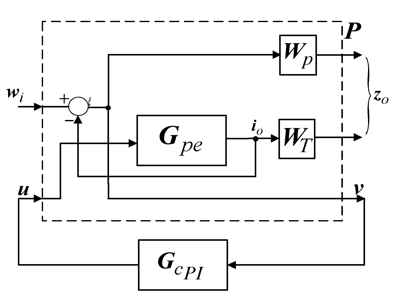
4. Generalized Representation and Controller Design

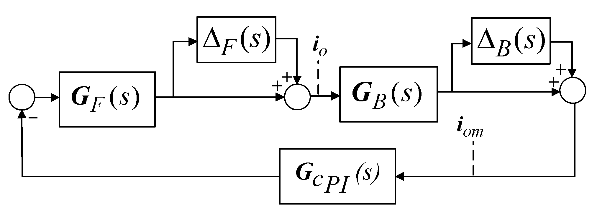
4.1. Generalized Representation

In this section, the verified transfer functions are used to translate the “inverter power exchange in weak-grid condition” problem into the framework of robust control. In this regard, a generalized representation of the inverter output dynamics is useful for analyzing and designing the robust inner-loop current controller. Therefore, the loops of the output stage of the inverter block diagram shown in Figure 6 are eliminated to produce the following equivalent transfer functions:

$${\mathit{G}}_F={\mathit{G}}_{PWM}{\mathit{G}}_{\mathit{D}{\mathit{i}}_o}{\left[\mathit{I}+{\mathit{Z}}_g\left({\mathit{Y}}_{ol}-{\mathit{G}}_{PLL}{\mathit{G}}_{\mathit{D}{\mathit{i}}_o}\right)\right]}^{-1}$$

(13)

$${\mathit{G}}_{\mathit{B}}=\left(-{\mathit{Y}}_{PLL}{\mathit{Z}}_g+\mathit{I}\right)$$

(14)

G_F and G_B relate the input to output dynamics, respectively, of the duty ratio to output current, i_o, and the output current to the measured output current,${\mathit{i}}_{om}$. Increases in Z_g are treated as a parametric uncertainty, which is useful for formulating the problem as a robust control problem.

The reduced block diagram, including the normalized uncertainties due to Z_g, i.e., ${\Delta }_F(s)$ and ${\Delta }_{\mathit{B}}(s)$, is shown in Figure 8. Note that Δ(s) represents the uncertainty normalized to the nominal plant (Z_g= 0), i.e.: $\Delta (s)=\left|\frac{{\mathit{G}}_{{\mathit{Z}}_g\ne 0}(s)-{\mathit{G}}_{{\mathit{Z}}_g=0}(s)}{{\mathit{G}}_{{\mathit{Z}}_g=0}(s)}\right|$.

To obtain the generalized plant configuration P of the system, Figure 8 is recast to that shown in Figure 9 with: ${\mathit{G}}_{pe}=\frac{{\mathit{G}}_F}{\mathit{I}+{\mathit{G}}_F{\mathit{G}}_{c_{P\mathit{I}}}\left({\mathit{G}}_{\mathit{B}}-\mathit{I}\right)}$, and ${\mathit{G}}_{c_{P\mathit{I}}}$ as the controller to be tuned. Note that the control signal u is not penalized and, therefore, the weighting is omitted from the generalized representation.

The exogeneous inputs to the generalized plant P are gathered in the input vector w_i = [${\mathit{i}}_{d_{ref}}$${\mathit{v}}_g$${\mathit{i}}_{in}$]^T, and the controller input to P is specified by u. The weighted exogeneous outputs of P are gathered in z_o = [$W_T{\mathit{i}}_o$ $W_{P}e$]^T, with W_T and W_P weighting functions as explained in Section 4.2. The output vector v is given by [e 0].

With these expressions, the generalized open-loop expression from [w_i u ]^T to [z_o v ]^T is given by,

$$\left[\begin{array}{c}{\mathit{z}}_o\\ \mathit{v}\end{array}\right]=\left[\begin{array}{cc}{\mathit{P}}_{11}& {\mathit{P}}_{12}\\ {\mathit{P}}_{21}& {\mathit{P}}_{22}\end{array}\right]\left[\begin{array}{c}{\mathit{w}}_{\mathit{i}}\\ \mathit{u}\end{array}\right]$$

(15)

where P is partitioned as follows:

$${\mathit{P}}_{11}=\left[\begin{array}{c}0\\ {\mathit{W}}_P\end{array}\right];{\mathit{P}}_{12}=\left[\begin{array}{c}{\mathit{W}}_T{\mathit{G}}_{pe}\\ -{\mathit{W}}_P{\mathit{G}}_{pe}\end{array}\right];{\mathit{P}}_{21}=\left[\mathit{I}\right];{\mathit{P}}_{22}=\left[-{\mathit{G}}_{pe}\right]$$

(16)

The closed-loop relation between the input and output vectors, respectively, w_i and z_o, is found by computing the linear fractional transformation of P and ${\mathit{G}}_{c_{P\mathit{I}}}$ as follows:

$\mathit{N}={\mathit{P}}_{11}+{\mathit{P}}_{12}{\mathit{G}}_{c_{P\mathit{I}}}{\left(\mathit{I}-{\mathit{P}}_{22}{\mathit{G}}_{c_{P\mathit{I}}}\right)}^{-1}{\mathit{P}}_{21}$, which results in,

$$\mathit{N}=\left[\begin{array}{c}{\mathit{W}}_T{\mathit{G}}_{pe}{\mathit{G}}_{c_{P\mathit{I}}}{\left(\mathit{I}+{\mathit{G}}_{pe}{\mathit{G}}_{c_{P\mathit{I}}}\right)}^{-1}\\ {\mathit{W}}_P\left(\mathit{I}-{\mathit{G}}_{pe}{\mathit{G}}_{c_{P\mathit{I}}}{\left(\mathit{I}+{\mathit{G}}_{pe}{\mathit{G}}_{c_{P\mathit{I}}}\right)}^{-1}\right)\end{array}\right]=\left[\begin{array}{c}{\mathit{W}}_T\mathit{T}\\ {\mathit{W}}_P\mathit{S}\end{array}\right]$$

(17)

The resulting vector N contains the expressions of both the weighted-complementary sensitivity and sensitivity transfer functions, referred to, respectively, by T and S. The expression given by N is used for synthesizing the robust controller by the mixed-sensitivity method, as discussed in the results section.

4.2. Weighting Functions

The weighting functions (which should be stable and proper functions [29]) can be viewed as the tuning knobs for synthesizing the robust controller. In the mixed-sensitivity tuning method, two weighting functions, W_T and W_p, are required for, respectively, T and S. The inverse of these weighting functions, i.e., |W_T|⁻¹ and |W_p|⁻¹, form upper bounds on the perturbed T and S in the frequency domain. The variation of Z_g creates a parametric uncertainty in T and S and is modelled as a multiplicative perturbation, as shown in Figure 8. If the block diagram in Figure 8 is redrawn to an equivalent block diagram, as shown below in Figure 10 below, a single perturbation ${\Delta }_{eq}(s)={\Delta }_F(s){\Delta }_B(s)$ is obtained.

It can then be easily deduced from Figure 10 that, in accordance with the small-gain theorem [29], if the H_∞ norm of Δ_eqT is satisfied, i.e., $\left|{\Delta }_{eq}(s)\mathit{T}(s)\right|<1$ where T is derived with respect to i_o, the system will be stable throughout the uncertainty margin ${\Delta }_{eq}(s)$.The weighting function W_T is a representation of ${\Delta }_{eq}(s)$ and forms an upper bound across the entire frequency range; therefore, the following requirement is made of W_T:

$$\overline{\sigma }\left\{{\Delta }_{eq}\left(j\omega \right)\right\}<\left|{\mathit{W}}_T\left(j\omega \right)\right|.$$

With $\overline{\sigma }\left\{{\Delta }_{eq}\left(j\omega \right)\right\}$, the largest singular value of ${\Delta }_{eq}(s)$.

W_p⁻¹ forms an upper bound on the perturbed sensitivity function S_Δ and contains the desired performance requirements. Based on the presented arguments, the following transfer functions were considered, respectively, for W_T and W_p:

$${\mathit{W}}_T(s)={\left(\frac{{\omega }_{W_T}^{-1}s+M_T{}^{-1/2}}{{\omega }_{W_T}^{-1}{\mathit{A}}_T{}^{1/2}s+1}\right)}^2;{\mathit{W}}_p(s)=\frac{M_p^{-1}s+{\omega }_{W_p}}{s+{\omega }_{W_p}{A}_p}$$

Values of M_T = 3 and M_p = 8 were chosen to provide good roll off at high frequency. A_T and A_p were chosen to be small non-zero values, i.e., 10⁻⁶, such as to obtain a Butterworth type filter characteristic. The bandwidths ꞷ_WT and ꞷ_WP were selected such that ꞷ_WP < ꞷ_L < ꞷ_WT, where ꞷ_L is the loop cross-over frequency. The requirement that |S+T|=I means that both S and T cannot be made less than I in the same frequency range. Therefore, their respective bandwidths should be sufficiently separated [29].

Hence, ꞷ_WP was selected to yield a closed-loop time constant of around 1 ms and ꞷ_WT was chosen to be 10⁴ rad/s. Bode plots of the obtained weights and several plots of S_Δ (as Z_g is increased) and ${\Delta }_{eq}(s)$ are shown in Figure 11.

5. Results

5.1. Synthesized Robust Controller

In the mixed-sensitivity approach, the H_∞ norm of (17) is minimized and, thus, the obtained controller provides robustness in that it is capable of maintaining the system stability (|W_TT|<1) and performance (|W_pS|<1) throughout the predefined uncertainty margin.

The so-called fixed-structure control synthesis is conducted in MATLAB by applying the structured H_∞ optimization method detailed in [30]. The vector N is computed by invoking the lft() function with the input arguments G_pe and ${\mathit{G}}_{c_{P\mathit{I}}}$. ${\mathit{G}}_{c_{P\mathit{I}}}$ is treated as a tunable fixed structured transfer function, while the variation of Z_g in G_pe is captured with the ureal function [31]. The outer-loop voltage controller ${\mathit{G}}_{{\mathit{v}}_{PI}}$ was designed to have a crossover frequency of 40 Hz, and the PLL a crossover frequency of 50 Hz. The performance of the tuned robust PI controller (RPI) was compared to that of a nominal PI controller (PI) tuned by the regular loop shaping method. The PI was tuned to have a 65° PM at a crossover frequency of 1/10 the switching frequency [32]. Below are the obtained controllers:

$$\begin{array}{cc}\hfill & RP{I}_d=RP{I}_q=\frac{1.8s+44}{s}; \mathrm{with} \mathrm{final} \mathrm{peak} \mathrm{gain}: 1.03; \hfill \\ \hfill & P{I}_d=P{I}_q=\frac{0.21s+484}{s}\hfill \end{array}$$

5.2. Sensitivity Analysis

In the sensitivity analysis, the uncertainty margin of the line inductance (L_g) is made to be in the range of 0 mH–20 mH. In this regard, the base case corresponds to the situation where L_g is smaller than 3 mH (SCR > 10) and weak grid conditions where L_g is made to be greater than 10 mH (SCR < 3). According to (12), the stability and performance of the injected virtual inertia current (${\widehat{\mathit{i}}}_{in}$) can be predicted by the Nyquist criterion of Y_o^clZ_g [25]. To illustrate the performance difference between the PI and RPI, the PLL crossover frequency is raised to 100 Hz. The resulting Nyquist plot of Y_o^clZ_g is shown in Figure 12 as the SCR is decreased from above 10 to below 2. It is evident from the Nyquist plot that the stability margins of the system with the PI (red loci) have larger sensitivity to decreases in the SCR than that of the system with RPI (blue loci). When the SCR is decreased from 2 to 1, the PM and gain margin (GM) of the system with PI decrease from, respectively, around 59° to 25°, and from around 11.1 dB to 4.8 dB. In comparison, the system with RPI has smaller changes in the stability margins, i.e.: the PM changes from around 66° to 41°, while the GM changes from around 13 dB to 6.8 dB. The stability margin achieved with RPI at a SCR of around 1 is similar to that achieved with PI at a SCR of 2.3. This indicates that the system with RPI can handle more than a 50% decrease in SCR than the system with PI.

The performance sensitivity of the system with the PI and RPI is further analyzed by considering the magnitude plot of the closed-loop transfer function from ${\widehat{\mathit{i}}}_{d_{ref}}$ to ${\widehat{\mathit{i}}}_o$, i.e., T, as the SCR is decreased as before. Increases in the magnitude of T are a good indicator of degradation of the system damping and, therefore, a good indicator of poor transient performance [29]. The magnitude plots of T are shown in Figure 13 for the system with PI (red) and RPI (blue). Comparison of the two plots shows larger changes in |T| for the system with PI (2.3 dB to 18.5 dB) than for the system with RPI (1.14 dB to 8.8 dB) for the same decrease in SCR. This observation confirms the results from the Nyquist plot of Y_o^clZ_g, i.e., there is higher performance sensitivity to changes in SCR for the system with PI than for the system with RPI.

5.3. Time Domain Simulations

Finally, both controllers are used to perform time domain simulations with the validated detailed switching model of the CFVSI from Section 2. The PLL is fixed at 50 Hz, while the SCR is decreased from the base case of above 10 to the weak grid case of below 2. A step current of 10 A is injected at t = 0.05 s through the DC-DC boost converter, as previously outlined. Figure 14 shows that in the base case, i.e., SCR > 10, both controllers achieve identical response performance. However, as can be seen in Figure 15 and Figure 16, the performance of the system with PI deviates from its nominal state as the SCR is decreased from the base case to the weak grid case. The response eventually becomes underdamped at SCR < 2, which is also visible in the initially distorted current waveforms in Figure 16. On the contrary, as shown in Figure 17 and the abc-waveforms in Figure 18, the system with RPI shows little performance degradation throughout the same SCR decrease. This is a satisfactory result as it shows that the robustly tuned inner-loop PI controller can maintain its nominal performance in a weak grid condition with a fast PLL.

6. Conclusions

Fast frequency changes in low inertia grids will require a high BW PLL for virtual inertia response, and this requirement will degrade the stability margins of the inverter system should the SCR become low enough to create a strong PLL-grid impedance coupling. To address this problem, the design of a robust inner-loop current controller of a current fed grid-tie inverter system was investigated. It was shown that:

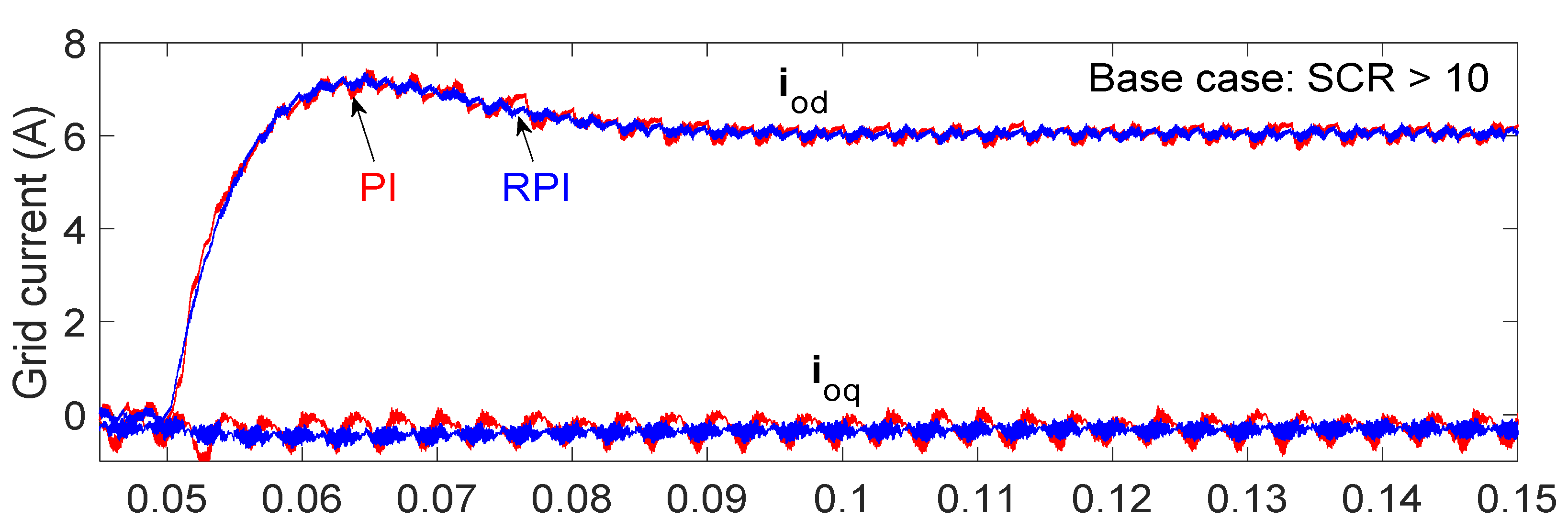
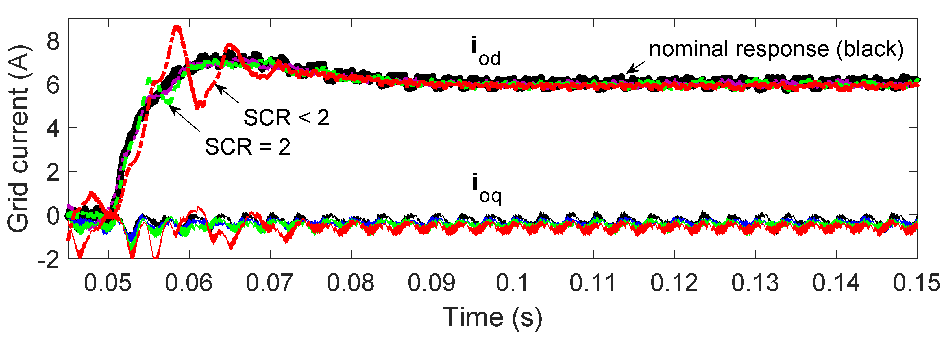
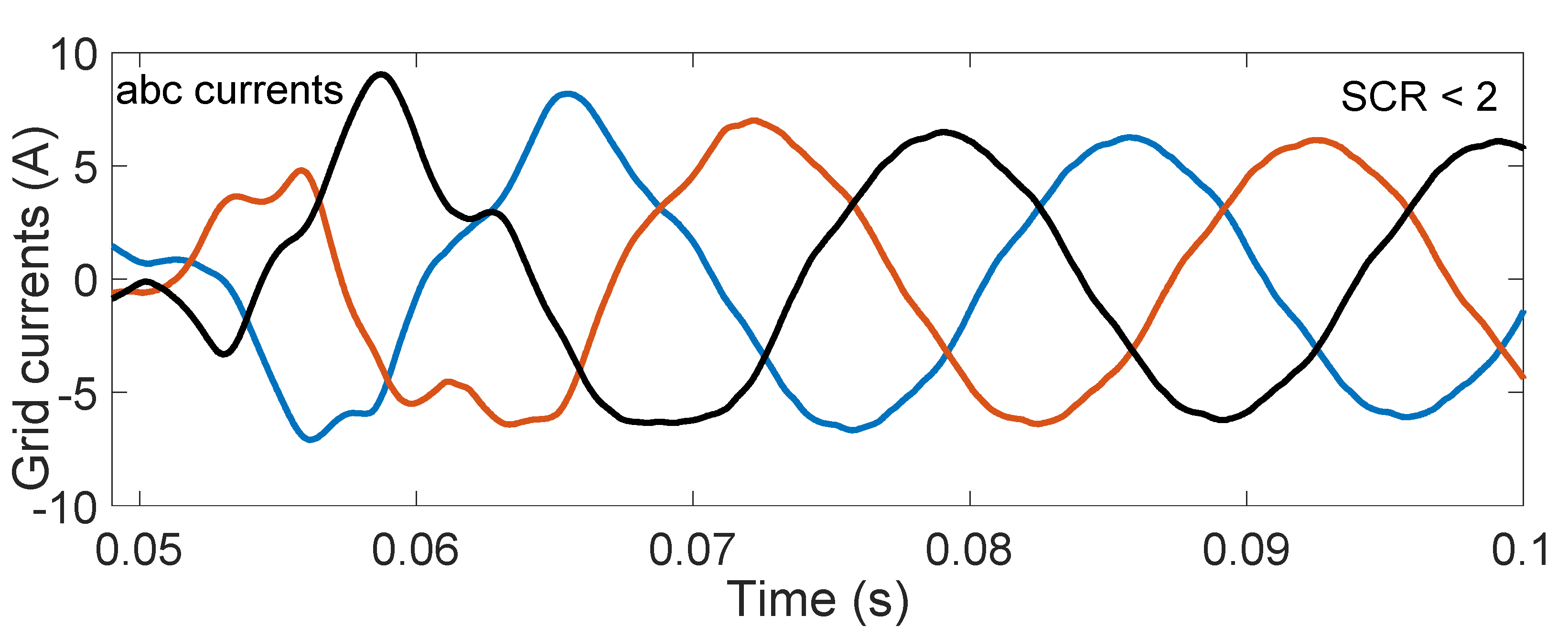
• While the regular loop-shaping method for tuning the inner-loop PI current controller is appropriate when the inverter-grid connection is strong (SCR > 10), it is inadequate in weak conditions (SCR < 3), even when the PLL-grid coupling dynamics are included in the loop transfer function.
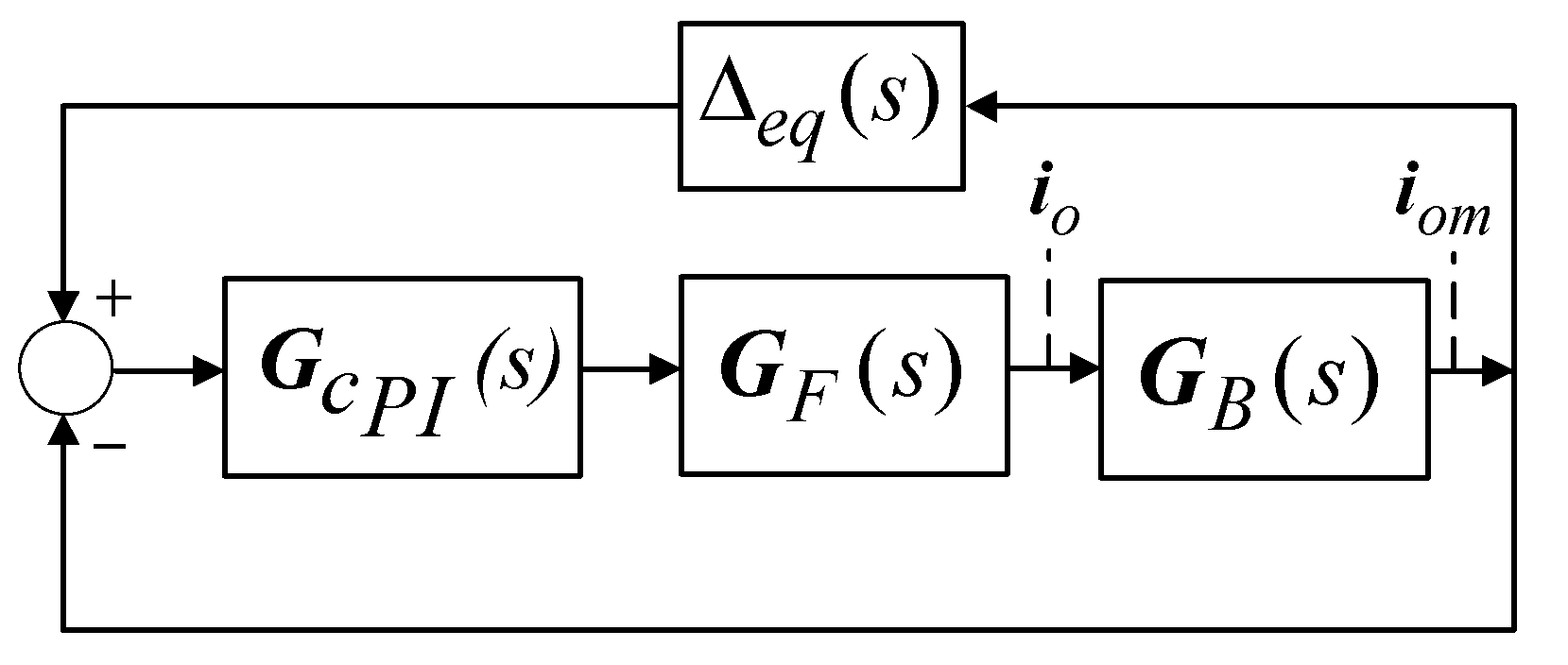
• The proposed alternative solution, whereby the PLL-grid coupling was formulated as a single perturbation on the dynamics of the inverter system, allowed for easy translation of the problem into the H_∞ robust control framework. Adequate inverter dynamics in the presence of a strong PLL-grid impedance coupling can then be achieved by tuning the controller to minimize the H_∞ norm.
• The structured H_∞ method [30] can be applied to tune the inner-loop PI controller against the PLL-grid impedance coupling, thereby avoiding an H_∞ controller with higher order dynamics.

Nyquist analysis and simulations with a validated model of a current fed grid-tie inverter confirmed that the performance of the inverter system with the H_∞ tuned PI controller was improved in the weak grid case of SCR < 3 as compared to the system with a regularly tuned PI controller. As future research, it would be useful to investigate whether inverter harmonic stability can be incorporated, formulated, and resolved in a similar manner.

References

1. Wright, P.S.; Davis, P.N.; Johnstone, K.; Rietveld, G.; Roscoe, A.J. Field Measurement of Frequency and ROCOF in the Presence of Phase Steps. IEEE Trans. Instrum. Meas. 2019, 68, 1688–1695. [Google Scholar] [CrossRef]
2. Sun, Y.; De Jong, E.C.W.; Wang, X.; Yang, D.; Blaabjerg, F.; Cuk, V.; Cobben, J.F.G. The Impact of PLL Dynamics on the Low Inertia Power Grid: A Case Study of Bonaire Island Power System. Energies 2019, 12, 1259. [Google Scholar] [CrossRef] [Green Version]
3. REE, Terna, TransnetBW, 50Hz, Transmission, Swissgrid, Energienet.dk. Frequency Stability Evaluation Criteria for the Synchronous Zone of Continental Europe; ENTSO-E: Brussels, Belgium, 2016. [Google Scholar]
4. DNV KEMA Energy & Sustainability. RoCoF An Independent Analysis on the Ability of Generators to Ride through Rate of Change of Frequency Values Up to 2 Hz/s; DNV KEMA Ltd: London, UK, 2013. [Google Scholar]
5. Yan, R.; Masood, N.-A.; Saha, T.K.; Bai, F.; Gu, H. The Anatomy of the 2016 South Australia Blackout: A Catastrophic Event in a High Renewable Network. IEEE Trans. Power Syst. 2018, 33, 5374–5388. [Google Scholar] [CrossRef]
6. ElectraNet. ESCRI-SA Battery Energy Storage—Final Knowledge Sharing Report; ElectraNet: Adelaide, Australia, 2021. [Google Scholar]
7. Hawaii Natural Energy Institute. Hawaii Natural Energy Institute Research Highlights Fast Frequency Response Battery on a Low-Inertia Grid. 2020. Available online: https://www.hnei.hawaii.edu/wp-content/uploads/Fast-Frequency-Response-Battery-on-a-Low-Inertia-Grid.pdf (accessed on 1 September 2021).
8. Vandermeer, J.; Glassmire, J.; Bitaraf, H.; Pike, C.; Wilber, M.; Whitney, E. Multi-Stage Flywheel Battery Energy Storage System at Chugach Electric Utility: A Performance Assessment. 2020. Available online: https://acep.uaf.edu/media/298261/MultiStage-Energy-Storage-System-Chugach_Final.pdf (accessed on 1 September 2021).
9. Goud, R.D.; Rayudu, R.; Mantha, V.; Moore, C.P. Impact of Short-circuit Ratio on Grid Integration of Wind Farms-A New Zealand Perspective. In Proceedings of the 2nd International Conference Large-Scale Grid Integration of Renewable Energy in India, New Delhi, India, 4–6 September 2019. [Google Scholar]
10. Zhang, C.; Wang, X.; Blaabjerg, F. Analysis of phase-locked loop influence on the stability of single-phase grid-connected inverter. In Proceedings of the 2015 IEEE 6th International Symposium on Power Electronics for Distributed Generation Systems (PEDG), Aachen, Germany, 22–25 June 2015; pp. 1–8. [Google Scholar]
11. Huang, Z. Revisiting Stability Criteria for DC Power Distribution Systems Based on Power Balance. CPSS Trans. Power Electron. Appl. 2017, 2, 76–85. [Google Scholar] [CrossRef]
12. He, Y.; Wang, X.; Ruan, X.; Pan, D.; Xu, X.; Liu, F. Capacitor-Current Proportional-Integral Positive Feedback Active Damping for LCL-Type Grid-Connected Inverter to Achieve High Robustness Against Grid Impedance Variation. IEEE Trans. Power Electron. 2019, 34, 12423–12436. [Google Scholar] [CrossRef]
13. JXu, J.; Qian, Q.; Xie, S. Adaptive control method for enhancing the stability of grid-connected inverters under very weak grid condition. In Proceedings of the 2018 IEEE Applied Power Electronics Conference and Exposition (APEC), San Antonio, TX, USA, 4–8 March 2018; pp. 1141–1146. [Google Scholar]
14. Jang, Y.; Erickson, R. Physical origins of input filter oscillations in current programmed converters. IEEE Trans. Power Electron. 1992, 7, 725–733. [Google Scholar] [CrossRef]
15. Huang, X.; Wang, K.; Fan, B.; Yang, Q.; Li, G.-J.; Xie, D.; Crow, M.L. Robust Current Control of Grid-Tied Inverters for Renewable Energy Integration Under Non-Ideal Grid Conditions. IEEE Trans. Sustain. Energy 2020, 11, 477–488. [Google Scholar] [CrossRef]
16. Wang, J.; Tyuryukanov, I.; Monti, A. Design of a novel robust current controller for grid-connected inverter against grid impedance variations. Int. J. Electr. Power Energy Syst. 2019, 110, 454–466. [Google Scholar] [CrossRef]
17. Xu, J.; Zhang, B.; Qian, Q.; Meng, X.; Xie, S. Robust control and design based on impedance-based stability criterion for improving stability and harmonics rejection of inverters in weak grid. In Proceedings of the 2017 IEEE Applied Power Electronics Conference and Exposition (APEC), Tampa, FL, USA, 26–30 March 2017; pp. 3619–3624. [Google Scholar]
18. Kaura, V.; Blasko, V. Operation of a phase locked loop system under distorted utility conditions. IEEE Trans. Ind. Appl. 1997, 33, 58–63. [Google Scholar] [CrossRef]
19. Yang, S.; Lei, Q.; Peng, F.Z.; Qian, Z. A Robust Control Scheme for Grid-Connected Voltage-Source Inverters. IEEE Trans. Ind. Electron. 2010, 58, 202–212. [Google Scholar] [CrossRef]
20. Gryning, M.P.S.; Wu, Q.; Blanke, M.; Niemann, H.H.; Andersen, K.P.H. Wind Turbine Inverter Robust Loop-Shaping Control Subject to Grid Interaction Effects. IEEE Trans. Sustain. Energy 2015, 7, 41–50. [Google Scholar] [CrossRef] [Green Version]
21. Wang, Y.; Wang, J.; Zeng, W.; Liu, H.; Chai, Y. H∞ Robust Control of an LCL-Type Grid-Connected Inverter with Large-Scale Grid Impedance Perturbation. Energies 2018, 11, 57. [Google Scholar] [CrossRef] [Green Version]
22. Osório, C.R.D.; Borin, L.C.; Koch, G.G.; Montagner, V.F. Optimization of Robust PI Controllers for Grid-Tied Inverters. In Proceedings of the 2019 IEEE 15th Brazilian Power Electronics Conference and 5th IEEE Southern Power Electronics Conference (COBEP/SPEC), Santos, Brazil, 1–4 December 2019; pp. 1–6. [Google Scholar]
23. Zhou, S.; Zou, X.; Zhu, D.; Tong, L.; Zhao, Y.; Kang, Y.; Yuan, X. An Improved Design of Current Controller for LCL-Type Grid-Connected Converter to Reduce Negative Effect of PLL in Weak Grid. IEEE J. Emerg. Sel. Top. Power Electron. 2018, 6, 648–663. [Google Scholar] [CrossRef]
24. Liserre, M.; Blaabjerg, F.; Hansen, S. Design and Control of an LCL-Filter-Based Three-Phase Active Rectifier. IEEE Trans. Ind. Appl. 2005, 41, 1281–1291. [Google Scholar] [CrossRef]
25. Messo, T.; Aapro, A.; Suntio, T. Generalized multivariable small-signal model of three-phase grid-connected inverter in dq-domain. In Proceedings of the 2015 IEEE 16th Workshop on Control and Modeling for Power Electronics (COMPEL), Vancouver, BC, Canada, 12-15 July 2015; pp. 1–8. [Google Scholar]
26. Wang, X.; Harnefors, L.; Blaabjerg, F. Unified Impedance Model of Grid-Connected Voltage-Source Converters. IEEE Trans. Power Electron. 2018, 33, 1775–1787. [Google Scholar] [CrossRef] [Green Version]
27. Harnefors, L.; Bongiorno, M.; Lundberg, S. Input-Admittance Calculation and Shaping for Controlled Voltage-Source Converters. IEEE Trans. Ind. Electron. 2007, 54, 3323–3334. [Google Scholar] [CrossRef]
28. The MathWorks, Inc. Simulink ® Control Design TM Getting Started Guide R2021a; The Mathworks, Inc.: Natick, MA, USA, 2021. [Google Scholar]
29. Skogestad, S.; Postlethwaite, I. Multivariable Feedback Control: Analysis and Design, 2nd ed.; Wiley: New York, NY, USA, 2007; Volume 2. [Google Scholar]
30. Gahinet, P.; Apkarian, P. Decentralized and fixed-structure H∞ control in MATLAB. In Proceedings of the IEEE Conference on Decision and Control and European Control Conference, Orlando, FL, USA, 12–15 December 2011; pp. 8205–8210. [Google Scholar]
31. Balas, G.; Chiang, R.; Packard, A.; Safonov, M. Robust Control Toolbox TM Getting Started Guide R2020b, 6.9; The Mathworks, Inc.: Natick, MA, USA, 2020. [Google Scholar]
32. Peña-Alzola, R.; Blaabjerg, F. Design and Control of Voltage Source Converters With LCL -Filters. In Control of Power Electronic Converters and Systems; Academic Press: Cambridge, MA, USA, 2018; pp. 207–242. [Google Scholar]
Figure 1. Lab-setup of CFVSI.
Energies 14 05546 g001
Figure 2. Schematic diagram of a typical current-fed voltage source inverter.
Energies 14 05546 g002
Figure 3. Current injection of 5 A at 5 A/s.
Energies 14 05546 g003
Figure 4. Current injection of 8A instantaneously.
Energies 14 05546 g004
Figure 5. Current injection of 10 A at 100 A/s.
Energies 14 05546 g005
Figure 6. Total system block diagram.
Energies 14 05546 g006
Figure 7. Frequency responses of Yocl. Red-dotted: estimation; blue solid line: transfer function.
Energies 14 05546 g007
Figure 8. Reduced block diagram.
Energies 14 05546 g008
Figure 9. Generalized representation of the system.
Energies 14 05546 g009
Figure 10. Simplified block diagram with single multiplicative perturbation.
Energies 14 05546 g010
Figure 11. Weighted upper bounds on Δeq(s) and SΔ(s).
Energies 14 05546 g011
Figure 12. Nyquist plot of YoclZg. Red: PI; blue: RPI.
Energies 14 05546 g012
Figure 13. Magnitude plots of |T|. Red: PI; blue: RPI.
Energies 14 05546 g013
Figure 14. dq-grid currents with SCR > 10. Red: PI; blue: RPI.
Energies 14 05546 g014
Figure 15. dq-grid currents of the system with PI for SCR < 10.
Energies 14 05546 g015
Figure 16. Grid current waveforms of the system with PI for SCR < 2.
Energies 14 05546 g016
Figure 17. dq-grid currents of the system with RPI for SCR < 10.
Energies 14 05546 g017
Figure 18. Grid current waveforms of the system with RPI for SCR < 2.
Energies 14 05546 g018