Empirical Correlations between the Hydraulic Properties Obtained from the Geoelectrical Methods and Water Well Data of Arak Aquifer

Abstract

A number of empirical correlations have been achieved between the hydraulic properties measured through geoelectrical methods and water well data of Arak Aquifer located in Markazi province, Iran. The geoelectrical method of Vertical Electrical Sounding (VES) technique was used to calculate the hydraulic properties of the aquifer. Through the VES technique, the pivotal hydraulic properties such as porosity, hydraulic conductivity, and specific yield of the layers were calculated. The results of VES technique were compared with the data obtained from seven observation water wells that were already drilled as exploratory coring boreholes in the region. The results demonstrate that as the porosity and hydraulic conductivity of the water-bearing layer increase, the results of VES technique appear much identical to the water well records. Furthermore, the specific yield was calculated as 4.6% that was very close to the value of 3.5% measured through the previous pumping tests. Moreover, VES technique predicted the water table of the aquifer very close to the water level monitored in the observation water wells. The obtained correlations can be used as an alternative for drilling of new observation wells that are inefficient in time and expense, and may encounter environmental limitations of drilling and site construction.

1. Introduction

About 30% of the world’s population depends on underground water, and more than 70% of groundwater resources are consumed by the agriculture sector. In Iran, a dramatic rise in water consumption has caused more exploitation, and faster extraction of underground water resources than the past. Therefore, the importance of studying groundwater for exploration, management and control of this valuable resource is increasing daily in the country.

One of the main goals of a hydrogeological study is determination of porosity, hydraulic conductivity, storativity and water transferability in the aquifer or underground rocks. These properties can be directly related to the electrical resistivity that is the basis of geoelectrical method. So far, the application of geoelectric method for determination of the aquifer characteristics has been widely developed in engineering, environmental and hydrogeological studies [1]. In the next sections, a number of applications of this method have been depicted.

Geoelectric sounding by Schlumberger method was used to determination of hydraulic parameters in the semi-arid areas of Jalore in northwestern India [2]. They used AIMRESI software to model the hydraulic and resistivity properties. The calculated resistivity was in a close compatibility with the regional data obtained from the water wells. The effect of pollution leak was investigated using Vertical Electrical Sounding (VES) technique in Moscow [3]. During that research, two polluted areas were determined using the VES technique. Additionally, properties such as resistivity together with porosity and clay content were adopted to typify the aquifer and aquitard. Geoelectric sounding by Schlumberger method was used for describing of the conditions of an aquifer situated in the semi-arid region of Khanasser valley, Syria, and compared to the hydraulic conductivity derived from pumping tests in the area. It was concluded that the hydraulic conductivity and permeability coefficient can be used for modeling and mapping the aquifer [4].

Resistivity property was used to estimate the aquifer hydraulic properties, and modeling the influences of pollutants on water quality within an aquifer in China [5]. The transmissivity of the geological formations in the study area also was estimated; it showed a wide range of the high inhomogeneity of the sedimentary formations together with the complexity of the karst formations. Based on the calculated hydraulic parameters, they made several hydrogeological maps, which were very useful for the modeling of contaminant migration. Resistivity, thickness, and lithology of the aquifer layers along with the fresh water quality were determined by the applied method [6].

VES technique was deployed to measure the hydraulic properties in an aquifer located in Iraq [7]. Using VES technique, an aquifer and bedrock in south Nigeria was successfully surveyed [8]. Schlumberger array was used in this research, and IPI2win software was applied to interpret the field data. The results of this study revealed three water-bearing layers. It was also found that the main aquifer was situated in the weathered and broken parts of the bedrock. Finally, using the 3-dimensional resistivity maps and hydraulic properties of the aquifer, the most appropriate locations for drilling of future water wells were identified. George et al. utilized the VES technique to calculate the hydraulic conductivity of the sediments in the coastal parts of Nigeria [9]. They could classify the sediments such as siltstones and sands based on their grain size. An application of their study was the usage of the results of VES method instead of the water well tests to quantify the hydraulic conductivity of the aquifer. In addition, they discovered two different aquifers in the region, and could characterize both of them. Contour maps of hydraulic conductivity, layer thickness and resistivity of the aquifers were also prepared [10].

Grain size distribution, together with the shape type of the salt water contamination in the coastal aquifers of Chaouia, Morocco, were determined by using the VES and Electrical Resistivity Tomography (ERT) profiles. The results showed that the length of the salt water penetration depended on the lithological nature of the aquifer formations [11].

The depth of seawater intrusion was determined by using VES technique within the coastal fresh water aquifer located in the southern part of Black Sea coastline in Romania. As seawater intrusion had caused major variations in the aquifer resistivity, simulation of the particular hydrogeological situations of the area became possible [12]. Gómeza et al. probed the hydrogeological properties of an aquifer located adjacent to Oruro, Bolivian Altiplano [13]. They managed to utilize an affordable and alternative approach to estimate the hydraulic properties of the aquifer. By utilization of the experimental linear correlations between properties of resistivity and hydraulic conductivity, other parameters such as aquifer thickness, along with the most suitable spots for drilling of water wells were determined.

Management of underground water supplies calls for a sufficient knowledge of the hydraulic properties of existing aquifers. Understanding of these properties contribute to determination of total volume of the underground water, numerical modeling of the water flow within the aquifer, site selection for drilling of suitable water wells, long-time planning for management and consumption of accessible water resources, etc. Moreover, using these properties, some undesirable outcomes of water extraction can be predicted and handled to effective and positive consequences. For instance, the extent of some negative impacts such as land subsidence, fault reactivation, or water level change due to the local seismic activities derived from the long-lasting water production and can be scientifically investigated if other supplementary data including poroelastic and strength properties of the rocks are also available. In situ stresses surrounding the porous rocks are referred to as the most effective factors in the fluid movement underground [14,15,16]. According to the poroelasticity theory, water extraction through the water wells affects the in situ stress by reduction in pore volume, and fractures’ closure [17,18]. Reversely, change of in situ stress influences on the pore deformations and may cause land subsidence, seismic activities and even water well blockage [19].

Hydraulic properties can be conventionally estimated through the water well tests. However, these tests may be sometimes unfeasible due to the much-needed cost and time as well as possible environmental restrictions. Arak aquifer is located near the Arak city in Markazi Province, Iran, and supplies the drinking water for the urban inhabitants.

In this study, 75 different sounding points were used to measure the thickness of different rock layers, rock resistivity and in situ water electrical conductivity within the aquifer. Then, porosity and hydraulic conductivity along with the transmissivity and specific yield of the different sediments were calculated. Afterwards, they were compared to the observed results from the data of seven water wells that were already drilled in the region. Those water wells were initially drilled as the exploratory boreholes and coring operation was done through them to characterize the underground formations in the area. In this study, based on the comparison between different hydraulic parameters, several empirical correlations were developed to correct the future VES measurements in the area. Moreover, the water table in the boreholes that recently function as the observation wells was compared to the water table determined by VES method.

The calculated hydraulic properties obtained from the VES method and water well data were very identical. In addition, the results illustrated that as the porosity of the rock layers increase, the correlations between the hydraulic properties achieved from both methods are much more precise than when they are computed for low values of porosity. This trend was quite evident for porosity and hydraulic conductivity of the rock layers in the aquifer. On the second hand, the average value of the aquifer specific yield was computed as 4.6% by VES method. Using previous pumping tests conducted by the client company, this value was calculated as 3.5%, confirming a good agreement between two methods. Moreover, regarding the predicted water table, both methods could estimate the water level in a very close range.

This study showed that VES technique can be a good alternative for water well tests to calculate the hydraulic properties of the aquifers. As the grain size of the layers approaches to the gravel and sand grains, the porosity and hydraulic conductivity of the underlying rock formations can be predicted more precisely. When environmental or financial restrictions govern the drilling of water wells, VES method can be a very effective and affordable method to indirectly measure the hydraulic properties of the rocks.

2. Materials and Methods

2.1. Project Description

The study area is located in the south part of Meyghan Desert in Markazi province, Iran. A number of 75 geoelectrical sounding points (to perform VES technique) were utilized to characterize the water aquifer. These sounding points were arrayed in seven profiles including A, B, C, D, E, F, G, H, and I expanded from the south towards the north direction. Furthermore, the data of seven observation wells that had been already drilled in the area were deployed to compare with the results of VES technique. Figure 1 shows the geographical and geological map of the area as well as the locations of sounding points and water wells. The water wells had been drilled as exploratory boreholes, although finally, they functioned as observation wells. Hence, some data such as porosity and hydraulic conductivity of the water-bearing rock layers within the aquifer had been already obtained directly from the cores taken during the drilling operation of the exploratory boreholes. After completion of the boreholes, they have been preserved as observation wells to monitor the water level continuously. The data related to the water wells have been summarized in Table 1.

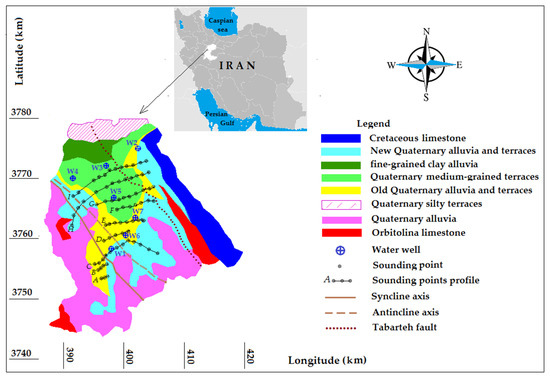
Figure 1. Geographical and geological map of the study area.

Table 1. Data of water wells. The values of porosity and hydraulic conductivity belong to the water-bearing rock layer in each water well within the Arak aquifer. k is hydraulic conductivity.

Well Name	X (m)	Y (m)	Z (m)	Water Table (m)	Water-Bearing Layer	Porosity (%)	k (cm/s)
W1	397,910	3,758,322	1781	1756	Clay-content alluvium	7.6	7.02
W2	402,329	3,774,972	1674	1652	Cretaceous limestone	8.7	6.90
W3	397,060	3,772,101	1673	1659	Fine-grained clay alluvium	29.0	3.10
W4	391,530	3,770,017	1674	1659	Quaternary sand terraces	19.5	5.30
W5	398,310	3,766,811	1696	1663	Quaternary sand terraces	16.1	9.20
W6	400,295	3,760,554	1753	1718	Clay-content alluvium	17.5	19.07
W7	401,887	3,763,508	1727	1665	Quaternary lime terraces	26.0	6.05

The aquifer is located in the Sanandaj-Sirjan zone and sub-zone of Haftad-ghole. The major fault of this region, which separated the two zones, is the Tabarteh fault, which is directed from the northwest to the southeast.

Alluvial deposits formed in the region are composed of coarse grains, medium grains, fine grains and very fine grains. The coarse grain formations are present in the east part of the area, and include rubble, sand and clay minerals. The type of those sediments is more calcareous and slate, and a little bit of igneous material, found in sandy-clay context. Moderate-grain alluvial deposits that cover most of the area include sand and gravel. The materials of these sediments are limestone and lime-slate stone which include more degree of clay content. The fine-grained alluvial sediments can be seen mostly in the eastern and southeast part of the desert in the area. The material of this type of alluvial has a lot of clay, with a small amount of sand grains. Very fine-grained sediments around the Meyghan Lake are seen in a narrow strip. These sediments were formed in the last stage of sedimentation and transportation of the rock particles by the occasional floods, and include a lot of clay, very fine sand and evaporate sediments such as gypsum and salt [20].

2.2. VES Technique Theory

Ohm’s law is the most fundamental physical law on which the theory of electrical resistivity is based, and can be expressed as:

$$J=\sigma E$$

(1)

where J represents the current density, σ represents the electrical conductivity of the environment, and E indicates the electric field strength of the environment. The resistivity, ρ, is equal to the inverse of conductivity, σ. In practice, what is measured is the voltage difference of the electric field. The relationship between the electric field strength and electric voltage is defined according to the following equation [21]:

$$E=-\nabla \left(\mathsf{\Phi }\right)$$

(2)

where Φ is the electric voltage. From Equations (1) and (2), it can be stated that:

$$J=-\sigma \nabla \left(\mathsf{\Phi }\right)$$

(3)

In a half-space ground, the relationship between the electric voltage and potential resistivity is defined as:

$$\mathsf{\Phi }=\frac{\rho I}{2\pi r}$$

(4)

where r is the distance of the desired electrode from the current source, Φ is the electric voltage, and I is the electric current.

Figure 2 shows an example of a four-electrode arrangement. In this figure, electrodes C₁ and C₂ represent the current electrodes while electrodes P₁ and P₂ represent the potential electrodes. This figure also shows how current is distributed, and how the electrical voltage is generated by the current.

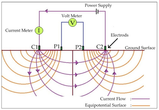
Figure 2. Distribution of the current lines and voltage.

The voltage generated by the two current electrodes at a given distance from a homogeneous and isotropic ground can be calculated as:

$$\mathsf{\Phi }=\frac{\rho I}{2\pi r}\left(\frac{1}{r_{c1}}-\frac{1}{r_{c2}}\right)$$

(5)

where, r_c1 is the distance of the desired point from the electrode C₁, and r_c2 indicates the distance of the same electrode from C₂. In this four-electrode arrangement, the voltage difference being created between the two voltage electrodes can be calculated as:

$$\Delta \mathsf{\Phi }=\frac{\rho I}{2\pi r}\left(\frac{1}{r_{c1p1}}-\frac{1}{r_{c2p1}}-\frac{1}{r_{c1p2}}+\frac{1}{r_{c2p2}}\right)$$

(6)

where $\Delta \mathsf{\Phi }$ is the voltage difference between the two voltage electrodes, r_c1p1 is the distance between the electrodes C₁ and P₁, r_c1p2 is the distance between the electrodes C₁ and P₂, and lastly, r_c2p2 is the distance between the electrodes C₂ and P₂. After measuring the voltage difference, the resistivity of the earth can be calculated as:

$${\rho }_a=K\frac{\Delta \mathsf{\Phi }}{I}$$

(7)

where ${\rho }_a$ is electrical resistivity of the earth, and K indicates the geometric factor used for the arrangement. K can be computed as:

$$K=2\pi {\left(\frac{1}{r_{c1p1}}-\frac{1}{r_{c2p1}}-\frac{1}{r_{c1p2}}+\frac{1}{r_{c2p2}}\right)}^{-1}$$

(8)

where K depends on how the four electrodes are arranged in each configuration. Resistivity-measuring devices usually measure the resistance of the ground. A number of researchers mentioned the underlying correlation between the ${\rho }_a$ and K as [21,22]:

$${\rho }_a=KR$$

(9)

An intriguing interpretation of VES technique in the field of hydrogeology can be found in [23].

2.3. Resistivity of Different Rocks

The rock resistivity is a function of rock porosity, cracks, saturation degree and the volume of insoluble salt compounds in the water [24]. The normal values of electrical resistivity for some rocks can be found in [25].

2.4. Estimation of Hydraulic Properties by VES Technique

VES technique can be used to estimate some hydraulic properties using relationships between electrical and hydraulic properties. For a water-saturated rock, Archie expresses the relationship between the resistivity of the rock, porosity, distribution and resistivity of the electrolyte [26]:

$${\rho }_r={\rho }_{w}a{\phi }^{-m}$$

(10)

where ${\rho }_r$ is the resistivity of rock mass (Ω·m) and ${\rho }_w$ represents the resistivity of the water in the formation (Ω·m). $a$ is a dimensionless adjustment coefficient. It is equal to 1 when the saturation degree is 100%. In this study, $a$ was assumed to be in the range between 0.3 and 1 for the different sediments. $\phi$ indicates the porosity, and $m$ represents the dimensionless coefficient of cementation which is relatively constant for a specific rock. m is also described as the pore-shape or grain-shape factor. The more cementation and compaction degree of the sediment, the higher value of m. In this study, based on the type of the regional sediments, the value of m was assumed to be equal to 1.5.

The electrical conductivity can be converted to the resistivity by the following equation:

$${\rho }_w=\frac{{10}^4}{E_w}$$

(11)

where $E_w$ is electrical conductivity of water (µS/cm), and can be calculated by interpolation of the water electrical conductivity in each location of the sounding points. Using Equation (11), the water resistivity,${\rho }_w$, for each sounding point is calculated. Then, using Equation (10), the spatial porosity of the aquifer can be determined.

Specific yield, $S_y$, of an aquifer is related to the resistivity of in situ water, ${\rho }_w$, the resistivity of the water-saturated rock layer, ${\rho }_{sat}$, the resistivity of unsaturated layer, ${\rho }_{unsat}$, and can be calculated using the following equation [27]:

$$S_y={\left(\frac{{\rho }_w}{{\rho }_{sat}}\right)}^{\frac{1}{m}}\left[1-{\left(\frac{{\rho }_{sat}}{{\rho }_{unsat}}\right)}^{\frac{1}{n}}\right]$$

(12)

In the current study, regarding the rock type of the layers, n = 2 was considered. Moreover, after estimation of the water table for each sounding point, the saturated and unsaturated layers were determined. In other words, the layers below and above the water table were considered as the saturated and unsaturated formations, respectively. Then, to obtain the bulk resistivity of a zone containing a group of saturated layers, the following equation was used:

$${\rho }_{sat}=\frac{{\sum }_{i=1}^n{h}_i{R}_i}{{\sum }_{i=1}^n{h}_i}$$

(13)

where ${\rho }_{sat}$ indicates the bulk resistivity of the saturated zone, n represents the number of layers in the zone, $R_i$ is the resistivity of the layer i, and $h_i$ represents the thickness of the i-th layer in the zone. Equation (13) was similarly used for calculation of bulk resistivity of a zone containing a group of unsaturated layers. In the next step, the values of $S_y$ for geoelectrical sounding points were calculated.

Hydraulic conductivity (m/s) is defined as the speed of water motion inside the porous rock. This parameter is a function of the rock and fluid (water) properties. The hydraulic conductivity for each layer can be calculated through the following relationship [28]:

$$k=\left(\frac{p_{w}g}{\mu }\right)\left(\frac{d^2}{180}\right)\left(\frac{{\phi }^3}{{\left(1-\phi \right)}^2}\right)$$

(14)

where d is the particle diameter (m) and $p_w$ represents the pore fluid density (1000 kg/m³). Parameter of g indicates the gravitation acceleration, $\phi$ is porosity, and μ is the fluid viscosity (0.0014 kg·ms).

As well as hydraulic conductivity property, transmissivity is also considered as one of the most important parameters that describes the fluid motion in the aquifer (Figure 3). In this figure, b and W are the thickness and width of the aquifer, respectively. Transmissivity is a function of the fluid (water) features, porous media (rock), and the rock layer thickness. Transmissivity incorporates the total saturation thickness whereas hydraulic conductivity indicates unit one. For definition of the transmissivity, a number of different approaches have been cited so far [29,30]. Fetter defined the transmissivity as the following equation [30]:

$$T=k·b$$

(15)

where T is transmissivity (m²/s), k is hydraulic conductivity (m/s), and b indicates the aquifer thickness (m).

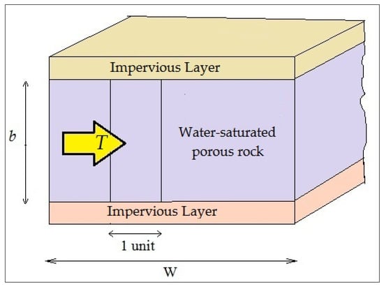
Figure 3. Transmissivity definition in a water-saturated porous medium.

3. Results and Discussion

In this study, the recorded data, obtained from 75 geoelectrical sounding points, were quantitatively interpreted using matching the curves to the Master curves. Then, for each sounding point, the number of rock layers, thickness, and resistivity were determined. Afterwards, the results obtained from the Master curves were imported as the primary data to the IX1D software. In the next step, the results were compared to the results derived from the modeling in IPI2win software. Finally, the results of those three methods (including IX1D software, IPI2win software, and Master curves) were analyzed and contrasted. For instance, Figure 4 shows the simulations in IPI2win software (a) and IX1D software (b) for geophysical sounding point E4.

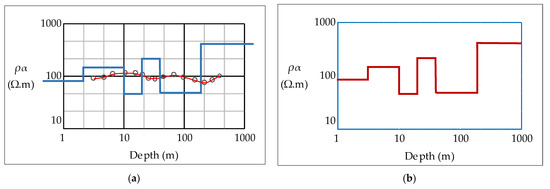
Figure 4. (a) Inverse modeling for sounding point E4 by IPI2win software. The field data is presented as the black points. The response of the model is in the form of a red curve while the inverse model is in the form of the blue line; (b) The model fitted to the sounding point E4 derived from the inverse modeling in IX1D software.

In the next step, for each sounding point, the results of the numerical modeling as well as the Master curves were compared. As an example, those results for sounding point E4 are presented in Table 2. The E4 sounding was situated in the center of the geoelectrical grid and the aquifer region. Hence, the results of E4 sounding point may reflect the typical range of the thickness and electrical resistivity of the sediments in the area.

Table 2. Results for the sounding point E4.

Layers	IPI2win		IX1D		Master Curves
Layer_id	t (m)	${\rho }_r$(Ω·m)	t (m)	${\rho }_r$(Ω·m)	t (m)	${\rho }_r$(Ω·m)
Layer_1	2.2	82	2.2	70	2.2	70
Layer_2	6.7	132	6.7	122	6.6	120
Layer_3	10	47	10	43	10	43
Layer_4	23	207	23	213	23	210
Layer_5	143	48	134	45	135	45

Figure 5 shows the 2D cross-section of the E profile that consisted of nine geoelectrical sounding points (E1–E9), which was performed in the Res2dinv software. In this profile, the upper horizon with a resistivity of 16 Ω·m to 200 Ω·m is composed from fine-grain and old alluvial sediments to the destructed granular grains’ layers. As shown, the range of the sounding point E1 has a high resistivity at very low depths—reason being that it is adjacent to the lime extrusion masses. In the interval between the sounding points E2 and E4, the elevation of the surface of the bedrock is also visible to some extent due to the anticline function. In this range, surface layers have high resistivity because of the presence of the coarse-grained sediments. In the range of sounding point E3, a water-bearing layer with a resistivity around 70 Ω·m is observed at the depth of 60 m. In the interval between the sounding points E4 to E5, an increase of thickness of the water-bearing layer with a resistivity between 30 Ω·m–60 Ω·m is visible, which is also confirmed through the interpretation of one-dimensional modeling results. In the range between the sounding points E6 to E8, the upraising of the surface of the bedrock and reducing of the thickness of the water-bearing layer can be easily seen. Finally, the vicinity of the sounding point E9 to the elevated calcareous masses demonstrates the absence of water-bearing layer within the interval of this sounding point.

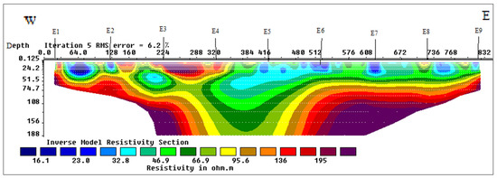
Figure 5. Two-dimensional cross-section obtained from inverse modeling for profile E.

Afterwards, through the comparison and combination of both 1D and 2D interpretations, the vertical profile of lithology was extracted for every sounding point. For instance, Figure 6 displays a typical profile for sounding point E4. Such profiles were deployed for calculation of saturated and unsaturated rock features for estimating the hydraulic properties.

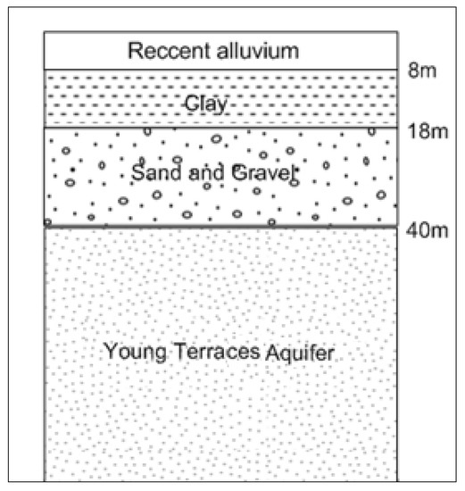
Figure 6. One-dimensional profile of the geophysical sounding point E4.

In this research, Surfer software was used to extract the contour maps of the hydraulic properties. For this purpose, firstly, the thickness and depth of the different rock layers for each sounding point (which was done by using numerical modeling in the previous step) were computed. Secondly, using the geoelectrical sounding locations and the depth of the rock layers, the contour maps were created in Surfer software. To this end, Kriging technique was chosen as the interpolation method. The contour depth map of the top of the basement layer derived from the one-dimensional interpretations is shown in Figure 7.

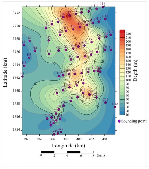
Figure 7. Contour depth map for bedrock obtained from the geoelectrical data of the study area.

One of the most useful applications of VES technique is the estimation of grain size of underground rock layers. Not only for aquifer studies, but also for a large number of other engineering phenomena where rock grain size plays a key role, can be utilized. For instance, regarding petroleum engineering, it may be used in hydraulic fracturing pre-studies [31,32].

In this study, through the geoelectrical interpretations, four different types of sediments were identified in the region. Based on the grain diameter, they were classified as the coarse-grained alluvium (d ≥ 0.50 mm), the medium-grained alluvium (0.01 mm ≤ d < 0.50 mm), the fine-grained alluvium (0.001 mm ≤ d < 0.01 mm), and the salty fine-grained alluvium (d < 0.001 mm). According to the Figure 8a, towards the desert located in the north of the area, the thickness of the coarse-grained alluvium gradually reduces. In Figure 8b, it can also be observed that the medium-grained alluvium in the central and northern parts have the highest thickness. Figure 8c indicates that the thickness of the fine-grained alluvium also increases towards the desert. In Figure 8d, the amount of the salty fine-grained alluvium which mostly consists of clay and salt increases towards the north of the plain.

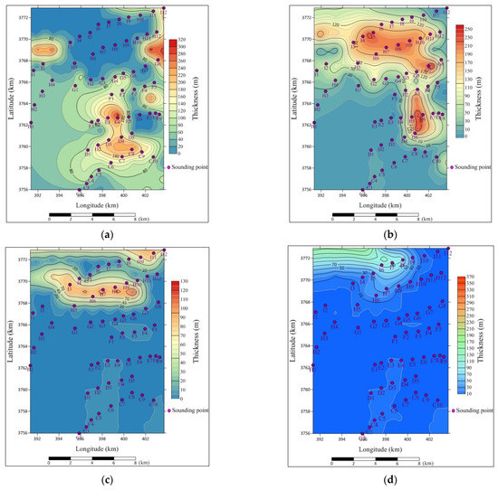
Figure 8. (a) Thickness contour map for coarse-grained alluvium; (b) Thickness contour map for medium-grained alluvium; (c) Thickness contour map for fine-grained alluvium; (d) Thickness contour map for salty fine-grained alluvium.

Figure 9 demonstrates the contour map of water electrical conductivity in the area. The values of groundwater electrical conductivity were interpolated using the soundings data and Kriging estimation method in Surfer. As it is observed, towards the desert, the water electrical conductivity builds up with increasing clay and fine-grained content as well as growing salinity of the water.

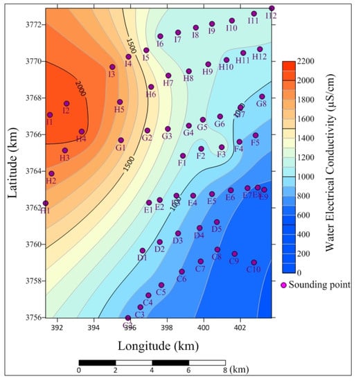
Figure 9. Contour map for groundwater electrical conductivity.

Using Equations (10)–(15), for each sounding point that detected a water-bearing layer in the subsurface, the properties of the water-bearing layer were calculated. Those properties included the resistivity of saturated rock, resistivity of unsaturated rock, the electrical conductivity of in situ water, water resistivity, rock porosity, specific yield, hydraulic conductivity and transmissivity; such calculated values are presented in Table 3.

Table 3. Calculated hydraulic properties for water-bearing layers at each sounding point.

Sounding	${\mathit{\rho }}_{\mathit{s}\mathit{a}\mathit{t}}$ (Ω·m)	${\mathit{\rho }}_{\mathit{u}\mathit{n}\mathit{s}\mathit{a}\mathit{t}}$ (Ω·m)	${\mathit{E}}_{\mathit{w}}$ (µS/cm)	${\mathit{\rho }}_{\mathit{w}}$ (Ω·m)	$\mathit{\phi }$ (%)	${\mathit{S}}_{\mathit{y}}$ (%)	$\mathit{k}$ (cm/s)	$\mathit{T}$ (m2/day)
C2	60	65	850	11.76	19.60	0.76	112	9.40
C3	62	74	830	12.04	19.43	1.64	2.31	9.53
C4	76	80	840	11.90	15.66	0.39	5.47	8.29
C5	82	140	850	11.76	9.72	0.68	8.62	4.89
C6	93	97	790	12.63	13.61	0.28	9.41	4.04
C7	81	92	736	13.58	16.77	1.03	23.0	4.006
C8	67	70	703	14.22	21.23	0.459	66.5	3.61
D1	100	113	1023	9.77	9.77	0.57	5.91	1.78
D2	98	154	966	10.35	10.56	2.13	3.44	3.20
D3	89	108	889	11.24	12.63	1.16	14.80	2.73
D4	64	67	795	12.57	19.65	0.44	24.70	3.02
D5	52	57	737	13.56	26.09	1.17	20.86	2.95
E3	80	100	1023	9.77	12.21	1.28	9.60	4.34
E4	68	96	928	10.77	15.84	2.50	13.91	3.14
E5	42	54	832	12.01	28.61	3.37	2.21	2.93
E6	37	38	769	13.00	35.14	0.46	7.23	2.06
E7	40	57	711	14.06	27.04	3.79	2.52	0.43
E8	60	63	688	14.53	24.22	0.58	27.71	0.80
F1	89	92	1127	8.87	9.64	0.16	4.47	2.98
F2	75	80	1047	9.55	12.73	0.40	9.63	7.11
F3	42	66	1212	8.25	19.64	3.97	68.30	7.55
F4	46	93	906	11.03	23.99	7.11	72.18	5.36
F5	66	111	884	11.31	17.13	3.92	50.16	4.54
G2	36	44	1458	6.85	15.58	1.64	8.70	0.43
G3	42	48	1304	7.66	18.25	1.179	10.94	1.68
G4	62	97	1165	8.58	13.84	2.77	2.79	3.96
G5	52	53	1111	9	17.30	0.16	4.78	6.80
G6	33	42	1038	9.63	29.19	3.31	35.41	5.10
G7	45	51	1001	9.99	22.2	1.34	10.36	1.26
G8	98	112	981	10.19	10.40	0.67	0.003	2.47
H1	70	83	1744	5.73	6.90	0.61	1.04	2.75
H4	67	73	2042	4.89	6.70	0.29	0.29	0.21
H5	40	42	1789	5.58	13.97	0.33	0.05	0.26
H6	21	31	1454	6.87	22.18	4.76	0.33	0.49
H7	15	38	1291	7.74	20.38	12.06	0.465	0.72
H8	18	32	1173	8.52	26.64	8.88	0.952	1.22
H9	19	33	1120	8.92	27.05	8.60	1.38	1.77
H10	20	41	1094	9.14	22.29	9.62	1.39	1.27
I3	15	31	1873	5.33	17.22	7.53	0.57	0.76
I4	12	21	1607	6.22	29.63	9.56	1.54	1.88
I5	17	25	1326	7.54	30.16	6.41	1.75	2.95
I6	18	31	1145	8.73	28.17	8.79	2.20	2.01
I7	20	30	1106	9.04	30.13	6.77	3.72	1.94
I8	21	28	1105	9.04	32.32	5.00	5.14	2.66
I9	17	42	1117	8.95	21.31	12.18	4.17	3.51
I10	22	60	1139	8.77	14.63	9.53	1.59	5.03
I11	38	78	1186	8.43	10.80	4.67	0.71	7.73
I12	47	94	1199	8.34	8.87	3.67	1.21	8.62

In the next step, using the obtained porosity values, the contour map of porosity was extracted for water-bearing layers in the aquifer (Figure 10). Since the depth of each water-bearing layer varied, the depth of the porosity contour map is variable. As it can be seen, the higher values of porosity are observed in the north of the region which is mainly composed of fine-grained alluvium deposits and clay. This is due to the presence of clay in the region. Sediments of clay materials due to the negative electrical charge of their particles cannot be well put together, and hence their porosity sometimes may reach up even to 60%.

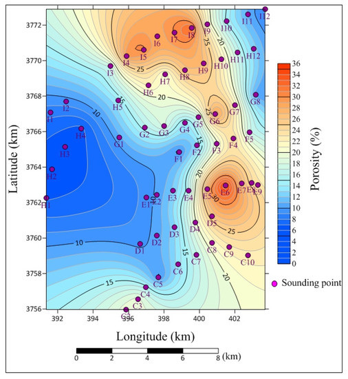
Figure 10. Contour map of porosity.

In the following section, the porosity and hydraulic conductivity of the water-bearing layers as well as the water table obtained from the VES technique are compared to the corresponding values gained from the water well data. Figure 11 demonstrates the porosity obtained from the VES technique versus water well data. As it can be seen, there is a good compatibility between the porosity values obtained through both approaches. The corresponding empirical correlation can be written as:

$${\phi }_{Well}=0.5{\left({\phi }_{VES}\right)}^{1.22}$$

(16)

where ${\phi }_{Well}$ and ${\phi }_{VES}$ are the porosity obtained from water well and VES technique, respectively.

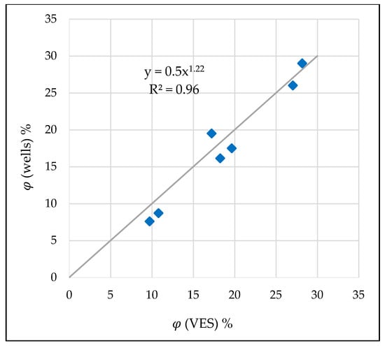
Figure 11. Porosity values obtained from VES method vs. water wells.

An important point that can be discovered from Figure 11 is that as the porosity of water-bearing layer increases, the estimation error for VES method decreases markedly. Figure 12 shows the percentage of estimation error in the calculation of porosity through the VES technique against the porosity achieved from the water wells. It is evident that as the porosity of the water-bearing layer increases, the estimation error decreases dramatically. Hence, it can be concluded that in high porosity layers, the calculated porosity from the VES technique is very close to the real value.

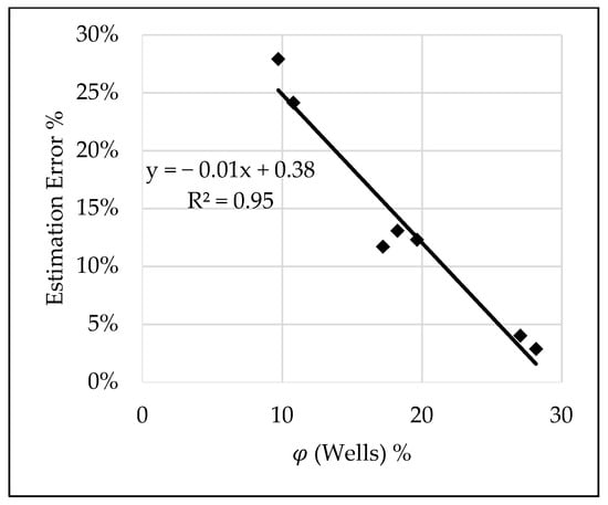
Figure 12. Percentage of the estimation error in calculation of porosity by VES technique.

Regarding the hydraulic conductivity, Figure 13 demonstrates the close relationship between both hydraulic conductivity calculated from the water wells and VES technique. The corresponding empirical correlation can be written as:

$$k_{Well}=0.02{\left(k_{VES}\right)}^2+0.08k_{VES}+5.24$$

(17)

where $k_{Well}$ and $k_{VES}$ are the hydraulic conductivity gained from the water wells and VES technique, respectively. Similar to the porosity, as the hydraulic conductivity of the rock increases, the value of the hydraulic conductivity estimated by the VES technique becomes closer to the water wells’ results.

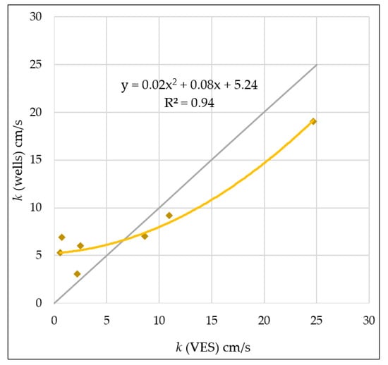
Figure 13. Hydraulic conductivity calculated by water wells vs. VES technique.

Finally, the efficiency of the VES method in estimation of water table was investigated. Figure 14 displays the water table predicted by the VES method versus real observations through the water wells. The obtained correlation confirms the similarity between the real water table and predicted values of water table by the VES method.

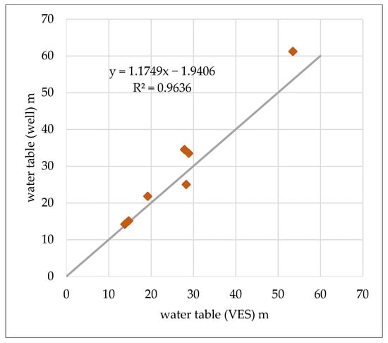
Figure 14. Water table predicted by the VES technique vs. real water table observed in water wells.

The hydraulic properties predicted by the VES technique are in a good agreement with the real data obtained from the water wells. As the porosity of the water-bearing layers increases, the results obtained from VES technique and water wells become closer. Porosity has a direct impact on the value of specific yield; thus, it is logical that the coarse-grained alluvium has the highest amount of storage coefficient in the area. In this study, for different geoelectrical sounding points, the specific yield values varied from 0.16% to 12.18%, which is related to clay, sand, sandstone, shale and limestone. Using the VES method, the average amount of the specific yield was determined equal to 4.6%. This confirms the average specific yield value of 3.5% measured by the client company during the prior pumping tests. In terms of the underground water utilization, the sedimentary rocks that have higher values of porosity and percentage of storage coefficient are preferred. The highest coefficient storage is for middle-grained to coarse-grained sediments. Hence, the best water-bearing layer is a layer that has both fine and coarse grains in the same extent. In terms of well drilling, neither clay layer nor very coarse grain layer is desirable; hence, the best proposed sites for drilling and water production are the locations of the H9, I4 and I7 sounding points.

Regarding the effect of granulation of rock particles, our results are similar to the study carried out by [33]. They concluded that the grain size distribution significantly influences on hydraulic conductivity and transmissivity of the aquifer. They found that in the presence of fine grains such as clay and shale, the hydraulic conductivity and transmissivity decline dramatically while coarse grains such as gravel and sand enhance those properties. In addition, the current research verifies their conclusion about the close correlation between the porosity and hydraulic conductivity of the water-bearing layers as well.

Similar to the works carried out by [9], the VES technique is quite efficient in time and expense to be as an alternative scenario for observation water wells to predict the water table. Additionally, it was found that VES technique can be easily applied to predict the vital hydraulic properties of the aquifer such as porosity, specific yield, hydraulic conductivity and transmissivity. Application of these techniques is offered strongly for developing the subjected aquifer, especially to avoid the environmental footprints in adjacent conservation areas.

Furthermore, combination of these hydraulic properties with poroelastic and strength features of the rocks can be a very beneficial tool to conduct numerical modeling of the whole aquifer system. Such simulations can help the engineers to detect the potential underground hazards threatening the aquifer life or water flow rate from the water wells for urban consumption. The reason is that due to the water extraction from the aquifer, the in situ stress regime governing the rock formations changes, and brings about small-scale or large-scale dynamic loadings which consequently influence the pore volume (porosity) of the aquifer [34].

4. Conclusions

In this study, the hydraulic properties of Arak aquifer were calculated through the Vertical Electrical Sounding (VES) technique. A number of 75 sounding points were installed on the aquifer ground, and some parameters such as the thickness of subsurface layers, rock resistivity and in situ water electrical conductivity were calculated. In the next step, the hydraulic properties such as porosity and hydraulic conductivity together with the transmissivity and specific yield of rock layers were determined. These results were compared to the values that were already obtained through the analysis of the core samples taken during the drilling operation of seven exploratory boreholes. Those boreholes functioned as observation wells during the conduction of this research and implementation of VES technique. Furthermore, the water table in the observation wells was compared to the water table predicted by VES technique.

Findings illustrate that VES technique and water well data provide close results so that some precise empirical correlations can be developed between them. For instance, the calculated porosity by VES technique is very close to the values obtained from the water well data. The results display that as the porosity of the layers is higher, the correlation is stronger, and the predicted values are more identical to the water well data. Furthermore, predicted hydraulic conductivity is also in a good agreement with the reported values of hydraulic conductivity through the water wells.

Additionally, it was found that the average specific yield of the aquifer is equal to 4.6% by VES technique which is close to the average specific yield value of 3.5% reported by the client company during the previous pumping tests’ measurements. Additionally, the water contour map (water table) provided through the VES technique, is very similar to the map acquired from the water wells. Hence, the application of VES and ERT techniques is strongly suggested to evaluate the aquifers especially when the physical limitations such as environmental regulations must be taken into account, and a more reasonable price of exploration activities is preferred.

References

- Kearey, P.; Brookes, M.; Hill, I. An Introduction to Geophysical Exploration, 3rd ed.; Wiley-Blackwell: Oxford, UK, 2002; ISBN 13 (EAN): 9780632049295. [Google Scholar]
- Yadav, G.S.; Aboalfazli, H. Geoelecteric sounding and their relationship to hydraulic parameters in semiarid regions of Jalore, northwestern India. Appl. Geophys. 1998, 39, 35–51. [Google Scholar] [CrossRef]
- Delgado-Rodríguez, O.; Shevnin, V.; Ochoa-Valdés, J.; Ryjov, A. Geoelectrical characterization of a site with hydrocarbon contamination caused by pipeline leakage. Geofísica Int. 2006, 45, 63–72. [Google Scholar] [CrossRef]
- Asfahani, J. Geoelectrical investigation for characterizing the hydrogeological conditions in semi-arid region in Khanasser valley, Syria. Arid Environ. 2006, 68, 31–52. [Google Scholar] [CrossRef]
- Pantelis, M.; Kouli, M.; Valliantos, F.; Vfidis, A.; Stavroulakis, G. Estimation of aquifer hydraulic parameters from surficial geophysical methods: A case study of Keritis Basin in Chania (Crete–Greece). J. Hydrol. 2007, 338, 122–131. [Google Scholar] [CrossRef]
- Arshad, M.; Cheema, J.M.; Ahmed, S. Determination of lithology and groundwater quality using electrical resistivity survey. Agric. Biol. 2007, 9, 143–146. [Google Scholar]
- Fadhil, A. The assessement of Erbil aquifer using geo-electrical investigation (Iraqi Kurdistan region). J. Appl. Sci. Environ. Sanit. 2009, 4, 43–54. [Google Scholar]
- Anuda, G.K.; Onuba, L.N. Geoelectric sounding for groundwater exploration in the crystalline basement terrain around Onipe and adjoining areas, southwestern Nigeria. Appl. Technol. Environ. Sanit. 2011, 1, 343–354. [Google Scholar]
- George, N.J.; Atat, J.G.; Umoren, E.B.; Isong, E.I. Geophysical exploration to estimate the surface conductivity of residual argillaceous bands in the groundwater repositories of coastal sediments of EOLGA, Nigeria. J. Astron. Geophys. 2017, 6, 174–183. [Google Scholar] [CrossRef]
- Are’touyap, Z.; Bisso, D.; Njandjock, N.P.; Amougou, M.L.E.; Asfahani, J. Hydrogeophysical characteristics of Pan-African aquifer specified through an alternative approach based on the interpretation of Vertical Electrical Sounding data in the Adamawa region, Central Africa. Nat. Resour. Res. 2019, 28, 63–77. [Google Scholar] [CrossRef]
- Alabjah, B.; Amraoui, F.; Chibout, M.M.; Slimani, M. Assessment of saltwater contamination extent in the coastal aquifers of Chaouia (Morocco) using the electric recognition. J. Hydrol. 2018, 566, 363–376. [Google Scholar] [CrossRef]
- Niculescu, B.M. Geophysical and geological investigations of the late Jurassic- early cretaceous aquifer in CernaVoda area, south Dobrogea (Romania). In Proceedings of the International Multidisciplinary Scientific GeoConference, Albena, Bulgaria, 30 June 2018. [Google Scholar] [CrossRef]
- Gómeza, E.; Bromana, V.; Dahlina, T.; Barmena, G.; Rosberga, J.E. Quantitative estimations of aquifer properties from resistivity in the Bolivian highlands. H2Open J. 2019, 2, 113–124. [Google Scholar] [CrossRef] [Green Version]
- Knez, D. Stress State Analysis in Aspect of Wellbore Drilling Direction. J. Arch. Min. Sci. 2014, 59, 71–76. [Google Scholar] [CrossRef] [Green Version]
- Knez, D.; Mazur, S. Simulation of Fracture Conductivity Changes due to Proppant Composition and Stress Cycles. J. Pol. Miner. Eng. Soc. 2019, 2, 231–234. [Google Scholar]
- Knez, D.; Calicki, A. Looking for a New Source of Natural Proppants in Poland. J. Bull. Pol. Acad. Sci. Tech. Sci. 2018, 66, 3–8. [Google Scholar] [CrossRef]
- Knez, D.; Rajaoalison, H. Discrepancy Between Measured Dynamic Poroelastic Parameters and Predicted Values from Wyllie’s Equation for Water-Saturated Istebna Sandstone. Acta Geophys. 2021, 69, 673–680. [Google Scholar] [CrossRef]
- Zamani, M.A.M.; Knez, D. A new mechanical-hydrodynamic safety factor index for sand production prediction. Energies 2021, 14, 3130. [Google Scholar] [CrossRef]
- Knez, D.; Wiśniowski, R.; Owusu, W.A. Turning Filling Material into Proppant for Coalbed Methane in Poland-Crush test results. Energies 2019, 12, 1820. [Google Scholar] [CrossRef] [Green Version]
- Mirzaei, M.; Ghadimi, A.F.; Gholami, S.; Adeshteh, V.; Baghri, A.; Mohseni, M.A. Determining hydrodynamics coefficients of AmanAbad aquifer using geoelectrical data. Hydrol. Eng. Geol. Geotech. 2011, 1, 421–428. [Google Scholar]
- Loke, M.H. Tutorial: 2D and 3D Electrical Imaging Surveys; Birmingham, UK, 2004; Available online: https://sites.ualberta.ca/~unsworth/UA-classes/223/loke_course_notes.pdf (accessed on 20 July 2021).
- Reynold, J.M. An Introduction to Applied and Environmental Geophysics, 2nd ed.; Wiley-Blackwell: Hoboken, NJ, USA, 2011; ISBN -13: 9780471485360. [Google Scholar]
- Atzemoglou, A.; Tsourlos, P. 2D interpretation of vertical electrical soundings: Application to the Sarantaporon basin (Thessaly, Greece). J. Geophys. Eng. 2012, 9, 50–59. [Google Scholar] [CrossRef]
- Klagari, A.A. Principles of Geophysical Exploration, 1st ed.; University of Tabriz Press: Tabriz, Iran, 1992. [Google Scholar]
- Telford, W.M.; Geldart, L.P.; Sheriff, R.E. Applied Geophysics, 2nd ed.; Cambridge University Press: Cambridge, UK, 1990; ISBN 9781139167932. [Google Scholar]
- Archie, G.E. The Electrical Resistivity Logs as and Aid in Determining some Reservoir characteristics. Pet. Technol. 1942, 146, 54–62. [Google Scholar] [CrossRef]
- Frohlich, R.K.; Kelly, W.E. Estimates of specific yield with the geoelectric resistivity method in glacial aquifers. J. Hydrol. 1987, 97, 33–44. [Google Scholar] [CrossRef]
- Domenico, P.A.; Schwartz, F.W. Physical and Chemical Hydrogeology, 2nd ed.; Wiley: Hoboken, NJ, USA, 1997; ISBN 978-0-471-59762-9. [Google Scholar]
- Freeze, R.A.; Cherry, J.A. Groundwater, 1st ed.; Prentice-Hall: Hoboken, NJ, USA, 1979; ISBN -13: 0-13-365312-9. [Google Scholar]
- Fetter, C.W. Applied Hydrogeology, 4th ed.; Pearson International Edition: London, UK, 2013; ISBN -13: 978-1292022901. [Google Scholar]
- Quosay, A.A.; Knez, D.; Ziaja, J. Hydraulic Fracturing: New Uncertainty Based modelling Approach for Process Design Using Monte Carlo Simulation Technique. PLoS ONE 2020, 15, e0236726. [Google Scholar] [CrossRef]
- Quosay, A.A.; Knez, D. Sensitivity Analysis on Fracturing Pressure using Monte Carlo Simulation Technique. Oil Gas Eur. Mag. 2016, 42, 140–144. [Google Scholar]
- Akhter, G.; Hasan, M. Determination of aquifer parameters using geoelectrical sounding and pumping test data in Khanewal District, Pakistan. Open Geosci. 2016, 8, 630–638. [Google Scholar] [CrossRef]
- Rajaoalison, H.; Knez, D.; Zlotkowski, A. Changes of Dynamic Mechanical Properties of Brine-Saturated Istebna Sandstone under Action of Temperature and Stress. Przemysł Chem. 2019, 98, 801–804. Available online: https://sigma-not.pl/publikacja-120236-2019-5.html (accessed on 22 May 2019).
Publisher’s Note: MDPI stays neutral with regard to jurisdictional claims in published maps and institutional affiliations. |
© 2021 by the authors. Licensee MDPI, Basel, Switzerland. This article is an open access article distributed under the terms and conditions of the Creative Commons Attribution (CC BY) license (https://creativecommons.org/licenses/by/4.0/).