A Minimal System Cost Minimization Model for Variable Renewable Energy Integration: Application to France and Comparison to Mean-Variance Analysis

Abstract

The viability of Variable Renewable Energy (VRE)-investment strategies depends on the response of dispatchable producers to satisfy the net load. We lack a simple research tool with sufficient complexity to represent major phenomena associated with the response of dispatchable producers to the integration of high shares of VRE and their impact on system costs. We develop a minimization of the system cost allowing one to quantify and decompose the system value of VRE depending on an aggregate dispatchable production. Defining the variable cost of the dispatchable generation as quadratic with a coefficient depending on macroeconomic factors such as the cost of greenhouse gas emissions leads to the simplest version of the model. In the absence of curtailment, and for particular parameter values, this version is equivalent to a mean-variance problem. We apply this model to France with solar and wind capacities distributed over the administrative regions of metropolitan France. In this case, ignoring the wholesale price effect and variability has a relatively small impact on optimal investments, but leads to largely underestimating the system total cost and overestimating the system marginal cost.

1. Introduction

Climate and energy action plans around the world set targets on the integration of large shares of Variable Renewable Energies (VREs), including wind and photovoltaic (PV) power (see, for instance, the 2030 Climate and Energy Framework of the European Union). Yet, increasing the penetration of VREs in electricity systems poses major challenges [1] and calls for the development of modeling tools to evaluate the technical feasibility and the economic viability of these objectives, as reviewed by Ringkjob et al. [2].

First among these challenges is the variable nature of VREs. They depend on meteorological conditions and thus pose challenges on the electricity system’s adequacy when conventional capacities are reduced Cretì and Fontini [3] (the system adequacy refers to the power system’s ability to meet the demand in the long-term, Chapter 22). Apart from scarcity periods, VRE generation can be abundant during other periods, which requires other generation technologies to reduce their output to avoid VRE curtailment. The combination of these impacts is referred to as utilization effect [4]. Furthermore, if markets respond as expected in the face of surplus supply, wholesale prices can be expected to fall (the so-called wholesale price effect). In addition, if VRE generation has to be curtailed at times of abundance, this will contribute to increased costs for the overall power system. This is referred to as the curtailment effect. The predictability of the VRE production is also limited and thus induces additional balancing needs. Moreover, VREs are location-specific, meaning that their production is not evenly distributed and that they cannot be transported like a fuel. Even though there is a large variability in the size of VRE projects, solar and wind energy harvesting is necessarily geographically dispersed. It is important to recognize that the development of VRE systems results from and produces a number of interactions between a number of actors such as citizens, electricity networks, markets, and ecosystems [5]. In this study, we do not address the political and social aspects of energy transformations. Instead, we concentrate on the integration of VRE to an existing interconnected system.

VREs deployment results in benefits and costs not only to the power system, but also to the wider economy and society. It is thus important to capture these costs and benefits appropriately. More specifically, while VREs have low marginal costs of generation, the above-mentioned characteristics induce system costs including adequacy costs, grid-related costs, and balancing costs [4]. A number of factors impact these costs: (i) the locational and temporal agreement between VRE generation and electricity demand, (ii) the distribution of VREs technologies and their penetration, (iii) the flexibility of the generation portfolio and the power system, and (iv) the capacity of the system to adapt to higher levels of VRE penetration over time. Yet, approaches based on Levelized Costs of Electricity (LCoEs) [3] (see Chapter 25.3, for a definition) alone do not account for these costs, as they depend on the rest of the electricity system. In particular, the LCoE does not take unavoidable correlations between the wholesale price of electricity and the VRE generation into account [6].

As reviewed in IEA [4] and Sijm [7], there are two main ways to take the effects of when, where and how VRE is generated into account in the economic assessment of a VRE technology: evaluating integration costs [8,9,10,11,12] or evaluating the System Total Cost (STC) [13,14,15]. For VREs, one can define the integration cost as the additional cost of adapting to higher VRE shares. These costs are calculated using modeling based on different scenarios. The technology for which the integration costs are to be calculated is included in a first scenario. In another scenario, the technology is excluded or included at a lower level of penetration. Using a number of techniques, the costs are computed for both scenarios and the difference is attributed to the technology in question. Yet, no standard recipe exists on which costs to include and on how to define the scenarios. This is a serious limit to the integration cost methodology [8]. In order to capture all relevant benefits and costs, another approach is to evaluate the STC of the entire power system. In this way, the system total or marginal value can be calculated to assess the impact of VREs integration on the STC [4]. The net benefit to the residual system, i.e., avoided costs minus increased costs, is given by the value of adding VRE generation. A positive value of additional VRE generation motivates further increasing the VRE penetration. From an economic perspective, any factor that contributes to reduce the VRE value constitutes an integration challenge. One major advantage of this methodology compared to the using integration costs is that it does not rely on a specific benchmark technology or on the segmentation of costs into different categories which are not clearly separated. In practice, however, sophisticated software are needed for both approaches in order to estimate the operation and investment costs of the power system. For instance, the family of EOLES models minimize the STC while satisfying energy demand of an energy system by optimizing investment and operation [16].

In order to go beyond VRE investment strategies based on the LCoE alone while avoiding having to model the rest of the power system, a number of authors have relied on the application of Markowitz’ mean-variance portfolio theory [17] to electricity systems. In these studies, a variance term is introduced in addition to the average VRE Capacity Factors (CFs) and fixed costs, which measures the variability of the total VRE production. This type of approach has the advantage to leave space for decision makers to find a trade-off between maximizing the expected renewable energy penetration or value and minimizing some risk measure which depends on the application. An overview of applications of mean-variance analysis to energy planning is provided by Brazilian and Roques [18] focusing on fossil fuel prices. There, investments are protected from price volatility by minimizing the financial risk. Mean-variance optimization based on levelized generation costs is used by Beltran [19] to derive the optimal VREs distribution in Mexico. In other works, the risk serves as a proxy for the reliability of the electricity system as VREs are introduced. For instance, weaker correlations between sites and sources can be leveraged to reduce the variance of the renewable energy production. This is the approach followed by Roques et al. [20] to optimize the distribution of wind power among five European countries. Their findings suggest that the European mix can be improved depending on the cost of variability. Using mean-variance analysis based on simulated daily-mean CFs on a 9 km grid, Thomaidis et al. [21] evaluate repowering actions based on solar and wind power in the southern Iberian Peninsula. The full Spanish wind mix is assessed by Santos-Alamillos et al. [22] using mean-variance optimization with ten years of simulated hourly wind CFs. Recently, Tantet et al. [23] apply mean-variance analysis to the study of the optimal recommissioning of VRE capacities in Italy using time series of both load and VRE CFs estimated from climate data. Bouramdane et al. [24] and Maimó-Far et al. [25] follow a similar approach to compare two different solar technologies in Morocco depending on the weight put on variability, and to analyze the role of the predictability of the photovoltaic (PV) production in Spain, respectively.

While mean-variance analysis is one of the simplest approaches to the problem of long-term investment in VRE accounting for the variability of the renewable energy generation, it lacks a rational to take an objective decision on the weight to put to the variance compared to the mean. Moreover, while the heuristic to maximize the mean penetration while limiting the variance seems sound, it is difficult to understand why one formulation of these terms should be favored to alternatives. In this article, we instead show how a particular form of mean-variance problem arises from an economic problem.

To focus on the investment in regional VRE capacities, the objective of this paper is to design a minimal long-term investment model taking into account the cost of the hourly conventional generation required to ensure the electricity system’s adequacy. Thus, we do not expect the model to be appropriate for operational studies. Rather, we require the program to be sufficient to conduct research works or pedagogical exercises aiming at revealing new or known effects stemming from the integration of large shares of VRE capacities in an electricity system, such as the wholesale price and utilization effects. This does not mean that the model could not be upgraded to include more realistic features to study more sophisticated effects stemming from the integration of VRE, but we leave such developments for future works.

By “minimal”, we mean that we aim at reducing the modeling of the conventional system to its bare minimum, while accounting for the fact that the integration of VREs impacts the cost of ensuring the system’s adequacy and that the marginal costs of peak conventional producers are larger than that of base producers. This second condition is particularly important as it is responsible for a non-trivial response of the pool of dispatchable producers to the variability of the VRE generation. To do so, our fundamental assumption is that the conventional producers are fully dispatchable and that we can approximate the total variable costs of the dispatchable producers by a convex function of the aggregate dispatchable generation only. This allows us to represent adequacy costs in a simple way, while neglecting grid-related, balancing, and flexibility costs. In addition, to concentrate on the integration of VRE capacities, we assume that the mix of dispatchable producers has a constant total capacity that is prescribed. This assumption is not fundamental and could be adjusted. Moreover, because we focus on the role of the variability of the renewable energy resource in the VRE value and adequacy costs, we only deal with the central-planning problem and leave the distributed market problem for future works. This leads to a two-stage quadratic recourse program in which the regional VRE capacities and the hourly dispatchable generation are optimized.

We give particular attention to a version of the problem for which quadratic dispatch variable costs are prescribed. This version is indeed the simplest version of the problem respecting the convexity condition of the dispatch variable costs. Moreover, this version is also interesting because it can be related to a particular mean-variance problem, as we show.

We also ask what are the adequacy costs arising from the variability of the renewable energy production in France depending on the dispatch variable costs and investigate the role of geographical and technological diversification. This question is interesting in itself and allows us to show how a numerical estimation of the model optimal solutions can be performed using a sample-average approximation. For this first case study, we assume that the load and the VRE CFs are stationary. While this assumption is questioned by expected changes in load patterns associated with the French climate-action plan [26] and with climate change [27], it does not prevent the identification of the wholesale price effect and of the emergence of adequacy costs depending on the VRE penetration.

In the next Section 2, we define a problem of investment in regional VRE capacities and generation dispatch based on a STC minimization simplified by the aggregation of the dispatchable generation and its costs. The precise mathematical framework in which we set this problem is described in Appendix A. We give merit-order and profit conditions for the optimality of solutions, which we prove in Appendix B. We also give two reduced versions of the problem against which solutions to the original problem can be compared to assess the impact of ignoring the wholesale price effect and variability when relying on LCoEs. We then show how to evaluate the VRE system total and marginal values together with adequacy costs in the model. Finally, a particular version of the model based on quadratic dispatch variable costs is presented. In Section 3, we describe a numerical version of the model based on a sample-average approximation using load and CF time series and configured for an application to the French electricity system. We analyze the results of this application in Section 4. After a description of the behavior of the model, we focus on the wholesale price effect and the role of variability as well as on the system value of VRE and adequacy costs. In Appendix C, we make sure that this analysis is robust to the sampling of the load and CF time series. Next, in Section 5, we show how the cost-minimization problem with quadratic dispatch variable costs relates to a particular version of mean-variance analysis with an adequate choice of parameters and compare their solutions in the case of France. We finish by summarizing this study and by discussing the range of potential applications of the model in Section 6.

2. Optimal Long-Term Investment Problem

A model of optimal long-term investment in VRE capacities taking adequacy costs associated with the variability of the VRE production into account is developed. It is based on the minimization of a STC including VRE rental costs and approximations of non-VRE-generation while treating non-VRE producers as an aggregate (lost load can be included in the STC using the value of lost load without major difficulties and will be used in another article).

2.1. Problem Definition

2.1.1. Defining the System Total Cost

Our objective is to define a STC reflecting adequacy costs stemming from the satisfaction of the load net of the VRE production by existing dispatchable producers. Approximating the costs by a function of the aggregate dispatchable generation only allows treating dispatchable producers as a single producer.

Conventional Mix

It is assumed that there is an initial mix of conventional (non-VRE) electricity producers which is able to meet an exogenous aggregate load at all hours (the loss-of-load probability is zero). The load is modeled by a one-year cyclostationary stochastic process ${\left(L\left(t\right)\right)}_{t\in \mathbb{T}}$. In other words, its statistics are stationary from one year to the next but depend on the hour of the year. ${\mathbb{T}}_0$ is the set of $T_0=8760$ h in a year (for non-leap years). For all practical purposes, it is assumed that the load is positive and attains a global minimum and a global maximum to which the total dispatchable generation capacity $x_{\mathrm{Di}}$ is identified (i.e., there is no load shedding). (The mathematical setting used here is presented in Appendix A, but the precise mathematical concepts and the stochasticity of the problem may be left aside for a first reading. In particular, it is assumed that the probability distribution of the load has a density. Its support is compact as it is bounded and closed.)

This initial mix is assumed to be fixed: $x_{\mathrm{Di}}$ remains unchanged even after the introduction of renewables. Moreover, these producers can dispatch energy at all times. They have no start-up, no-load, or ramp costs, and no must-run or minimum up/down-time requirements [28]. The only constraints are that their aggregate generation, represented by the non-negative stochastic process ${\left(G_{\mathrm{Di}}\left(t\right)\right)}_{t\in \mathbb{T}}$, should be positive (no storage) and no larger than their total generation capacity $x_{\mathrm{Di}}$.

In this setting, it is assumed that the distribution of the non-VRE producers results in an aggregate cost function of the form

$$\begin{array}{cc}\hfill {\mathrm{C}}_{\mathrm{Di}}\left(q\right)& ={\mathrm{FC}}_{\mathrm{Di}}+{\mathrm{VC}}_{\mathrm{Di}}\left(q\right)\hfill \end{array}$$

(1)

for some total quantity q to be produced. The non-negative constant ${\mathrm{FC}}_{\mathrm{Di}}$ (€) and the function ${\mathrm{VC}}_{\mathrm{Di}}$ (€) are the fixed cost and the variable cost of the dispatchable generation, respectively. (The variable-cost function ${\mathrm{VC}}_{\mathrm{Di}}$ is assumed to be non-negative, strictly convex, and differentiable over the real numbers, so that this is also true for the total cost function ${\mathrm{C}}_{\mathrm{Di}}$. It is also assumed that it is equal to 0 if $q=0$, with no loss of generality.) This aggregate cost function does not include grid-related costs associated with the electricity network extension, operation, and management. Moreover, the fixed cost of the dispatchable generation plays no role in this study on the optimization of VRE capacities for a prescribed dispatchable capacity. We anticipate that the introduction of VRE will result in a decrease in the dispatchable generation leading to a reduction of both the expected variable cost and the expected revenue for the dispatchable generation.

Introducing VRE

Next, m VRE producers indexed by i in $\{0,\dots ,m-1\}$ enter the system. For instance, each VRE producer may be associated to the total production by a given technology in a given region. Each producer has an exogenous CF given by the non-negative cyclostationary stochastic process ${\left(H_i\left(t\right)\right)}_{t\in \mathbb{T}}$ (the probability distribution of $H_i\left(t\right)$ is assumed to have a compact support, e.g., between 0 and 1, and to have a density). The collection of CFs is the multivariate stochastic process ${\left(\mathit{H}\left(t\right)\right)}_{t\in \mathbb{T}}$. For a given capacity $x_i$, the VRE producer i generates $x_i{H}_i(t,\omega )$ at time t and for some outcome $\omega$ in $\mathsf{\Omega }$. With $\mathit{x}=(x_0,\dots ,x_{m-1})$, the vector of VRE capacities the total VRE generation is given by

$$Q_{\mathit{x}}(t,\omega )=\sum _{i=0}^{m-1}{x}_i{H}_i(t,\omega ).$$

It is assumed that only fixed costs are incurred by VRE producers as the sum of annualized capital costs and fixed Operation and Management (O&M) costs. (O&M costs of VREs may depend on the number of operating hours. However, cost data often rely on the assumption that the number of operating hours is constant and O&M costs are considered as fixed costs [29].) The cost of the VRE producer i over one hour at any given time is, with certainty,

$${\mathrm{C}}_i\left(\mathit{x}\right)={\mathrm{hRC}}_i{x}_i={\mathrm{C}}_i\left(x_i\right),i\in \{0,\dots ,m-1\},$$

where ${\mathrm{hRC}}_i$ is the hourly rental cost of producer i. The the one-year total VRE cost is

$$\begin{array}{c}\hfill {\mathrm{C}}_{\mathit{x}}=T_0\sum _{i=0}^{m-1}{\mathrm{C}}_i\left(x_i\right)=T_0{\mathbf{hRC}}^T\mathit{x},\end{array}$$

(2)

where ${\mathbf{hRC}}^T$ is the transpose of the vector of VRE hourly rental costs $\mathbf{hRC}=({\mathrm{hRC}}_0,\dots ,$ ${\mathrm{hRC}}_{m-1})$. This cost is constant in time and only depends on the vector $\mathit{x}$ of installed VRE capacities.

Each hour, the conventional producers are assumed to be able to react instantaneously to varying loads and to generate at a variable cost ${\mathrm{VC}}_{\mathrm{Di}}$ (Equation (1)) that only depends on the instantaneous total dispatchable generation. Thus, no balancing is needed for this system to compensate for uncertainties in the short-term prediction of the CFs and the load.

The one-year STC with VREs is then

$$\begin{array}{c}\hfill \mathrm{STC}\left(\mathit{x},{\left(G_{\mathrm{Di}}(t,\omega )\right)}_{t\in {\mathbb{T}}_0}\right)={\mathrm{C}}_{\mathit{x}}+\sum _{t=0}^{T_0-1}{\mathrm{VC}}_{\mathrm{Di}}\left(G_{\mathrm{Di}}(t,\omega )\right)\end{array}$$

(3)

for some outcome $\omega \in \mathsf{\Omega }$. The aggregate dispatchable generation ${\left(G_{\mathrm{Di}}\left(t\right)\right)}_{t\in \mathbb{T}}$ is a key variable here, as it is through it that the conventional system responds to the introduction of VRE. This representation of the STC includes adequacy costs while ignoring grid-related costs and balancing costs. It takes the costs from the VRE producers and the dispatchable producers into account, and thus allows for the evaluation of the cost of satisfying the load, as opposed to an analysis based on the LCoEs only.

2.1.2. System Total Cost Minimization Problem

The optimal distribution $\overline{\mathit{x}}$ of VRE capacities, fixed in time, is looked for so as to minimize the expected one-year STC, Equation (3). (Because of the cyclostationarity of the load and CFs, the expectation of a cost over a year is equal to the expectation of that cost for subsequent years and does not depend on the initial hour of the year.) Network constraints are ignored and so are imports and exports. That is, it is assumed that the network is a copper plate with no transfer limits and closed from neighboring areas. The corresponding optimization problem is the two-stage quadratic recourse program [30] (Chapter 2.3):

$$\begin{array}{cc}\hfill \underset{\mathit{x}}{\min }& \mathbb{E}\left(\overline{\mathrm{STC}}\left(\mathit{x}\right)\right)\hfill \\ \hfill \mathrm{s}.\mathrm{t}.& x_i\le x_i^{\max },\hfill & \hfill & i\in \{0,\dots ,m-1\}\hfill \\ \hfill & x_i\ge 0,\hfill & \hfill & i\in \{0,\dots ,m-1\},\hfill \end{array}$$

(4)

where the recourse function $\overline{\mathrm{STC}}(\mathit{x},\omega )$ is the optimal value of the second-stage, or scheduling, problem:

$$\begin{array}{cc}\hfill \underset{{\left(G_{\mathrm{Di}}(t,\omega )\right)}_{t\in {\mathbb{T}}_0}}{\min }& \mathrm{STC}\left(\mathit{x},{\left(G_{\mathrm{Di}}(t,\omega )\right)}_{t\in {\mathbb{T}}_0}\right)\hfill \\ & \mathrm{s}.\mathrm{t}.G_{\mathrm{Di}}(t,\omega )+Q_{\mathit{x}}(t,\omega )\ge L(t,\omega )\hfill \\ \hfill & G_{\mathrm{Di}}(t,\omega )\le x_{\mathrm{Di}}\hfill \\ \hfill & G_{\mathrm{Di}}(t,\omega )\ge 0.\hfill \end{array}$$

(5)

This two-stage problem is referred to as the variable problem. The first stage is the long-term investment problem and is coupled with the generation scheduling problem of the second stage, i.e., the short-term problem in economics. We call the first constraint of the scheduling problem the adequacy constraint. It is this constraint that ensures that enough dispatchable energy ${\left(G_{\mathrm{Di}}\left(t\right)\right)}_{t\in \mathbb{T}}$ is generated to meet the residual load. The other constraints ensure that the total dispatchable generation remains positive and does not exceed the total dispatchable capacity. In the applications considered here, the latter is fixed to the maximum load so that optimal solutions will not activate this constraint, which we can safely ignore in the following.

The VRE generation is thus allowed to be curtailed at no extra cost. In other words, one may have $Q_{\mathit{x}}(t,\omega )>L(t,\omega )$ for some times and outcomes. The VRE capacities are also constrained in the investment problem (Equation (4)) not to be larger than a given positive maximum distribution per region and technology, $x_i^{\max }$, i in $\{0,\dots ,m-1\}$. Here, the VRE capacities are invested in starting from a mix without VRE, but the model could easily be adapted to an investment in additional VRE capacities.

The VRE capacities are the decision variables of the investment problem. The dispatchable generation at the different hours of the year are the decision variables of the scheduling problem. Because the load and the CFs introduce uncertainty in the scheduling problem, the optimal dispatchable generations are random. In practice, one can use a sample-average approximation to solve this problem numerically using time series for the load and the VRE CFs. Theorem 5.4 in Shapiro et al. [30] provides a pointwise version of the law of large numbers to show the consistency of optimal solutions and values of two-stage problems such as considered here [31] (Chapter 9). As discussed in Appendix A, even if the conditions of this theorem would be verified, one would still need to make sure that low-frequency variability and climate change on long time scales are sufficiently weak for the sample means to converge to an acceptable precision for the number of years available in the data. Thus, to support the robustness of the results of the application presented in Section 4, we prefer to numerically evaluate the convergence of the solutions with the length of the available time series in Appendix C.

2.2. Optimal System Marginal Cost and Profits

Necessary conditions that the optimal solutions of the cost-minimization problem (Equation (4)) must satisfy are now given.

Let the marginal cost, $c_{\mathrm{Di}}\left(q\right)={\mathrm{VC}}_{\mathrm{Di}}^{\prime }\left(q\right)$, of the dispatchable production be a strictly increasing function of the generation $q\ge 0$. The potential one-year profit per unit of installed capacity (€/MW) of the VRE producer i is given by. (We refer to this quantity as the profit in relationship to the problem of perfect markets even though the notion of profits is misleading in the centralized problem considered here.)

$$\mathbb{E}\left(\sum _{t=0}^{T_0-1}\lambda \left(t\right)H_i\left(t\right)\right)-T_0{\mathrm{hRC}}_i.$$

where $\lambda \left(t\right)$ (€/MW), is the (random) Karush-Kuhn-Tucker (KKT) multiplier of the adequacy constraint in the scheduling problem (Equation (5)) for some time t in ${\mathbb{T}}_0$. It is the System Marginal Cost (SMC) of electricity, i.e., the cost for the electricity system of serving one more unit of load [3] (Chapter 8). In a perfectly competitive wholesale electricity market, it would correspond to the equilibrium price of electricity per unit of energy [3] (Chapter 10).

To simplify the notations, we denote by $\langle X\rangle$ the expectation of the one-year average $\mathbb{E}(1/T_0{\sum }_{t=0}^{T_0-1}X\left(t\right))$ of some process X and refer to it simply as the average of X. Dividing by the CFs and assuming that the average SMC is positive, the one-year potential profits can be expressed per MWh produced as

$${\mathrm{P}}_i=\langle \lambda \rangle {\nu }_i-{\mathrm{LCoE}}_i,$$

(6)

in terms of value factor

$$\begin{array}{c}\hfill {\nu }_i=\frac{\langle \lambda H_i\rangle }{\langle \lambda \rangle \langle H_i\rangle },\end{array}$$

(7)

and LCoE (€/MW)

$$\begin{array}{c}\hfill {\mathrm{LCoE}}_i=\frac{{\mathrm{hRC}}_i}{\langle H_i\rangle },\end{array}$$

(8)

of the VRE producer i. We prove the following result in Appendix B.

Theorem 1.

For a given VRE mix $\mathit{x}$, the dispatchable generation $\overline{G_{\mathrm{Di}}}$ and the SMC $\overline{\lambda }$ make an optimal (primal/dual) solution of the scheduling problem (Equation (5)) only if, for all t in ${\mathbb{T}}_0$,

$$\begin{array}{cc}\hfill \mathrm{when}& x_{\mathrm{Di}}>L(t,\omega )-Q_{\mathit{x}}(t,\omega )>0:\hfill \\ \hfill & \left\{\begin{array}{cc}\overline{G_{\mathrm{Di}}}(t,\omega )\hfill & =L(t,\omega )-Q_{\mathit{x}}(t,\omega ),\hfill \\ \overline{\lambda }(t,\omega )\hfill & =c_{\mathrm{Di}}(L(t,\omega )-Q_{\mathit{x}}(t,\omega )),\hfill \end{array}\right.\hfill \\ \hfill \mathrm{when}& L(t,\omega )-Q_{\mathit{x}}(t,\omega )<0:\hfill \\ \hfill & \left\{\begin{array}{cc}\overline{G_{\mathrm{Di}}}(t,\omega )\hfill & =0,\hfill \\ \overline{\lambda }(t,\omega )\hfill & =0.\hfill \end{array}\right.\hfill \end{array}$$

(9)

Moreover, if the VRE mix $\overline{\mathit{x}}$ is an optimal solution of the investment problem (Equation (4)), then

• either the VRE producer i have a negative potential profit and no capacity is installed, $\overline{x_i}=0$, or
• the VRE producer i makes a non-negative profit and capacity is installed, $\overline{x_i}>0$. In this case,

  –

  either its profit is zero and its capacity is not capped, $0\le \overline{x_i}\le x_i^{\max }$ (the bounds may be reached but the corresponding constraints are inactive), or

  –

  i’s profit is positive (economic rent) and its capacity is maximal, $\overline{x_i}=x_i^{\max }$.

It follows that, at the optimum, the SMC at time t and for some outcome $\omega$ is a function of the residual load, $L(t,\omega )-Q_{\overline{\mathit{x}}}(t,\omega )$, only. This is illustrated in Figure 1.

When there is curtailment, the optimal SMC is given by the marginal cost of VRE production, which is zero here. Otherwise, the SMC is given by the marginal cost of the dispatchable generation, in agreement with standard merit-order dispatching [3] (Chapter 8).

2.3. Two Reduced Models Ignoring VRE Variability

Our goal is here to compare optimal solutions of Problem (4) with that from problems in which VRE variability is ignored. These problems help identify the contribution from variability to adequacy costs. The first ignores both variability and the impact of VRE generation on the SMC, while the second captures the effect of the average VRE generation on the SMC.

2.3.1. Decoupled Problem

First, the dispatch variable costs are assumed linear in the dispatchable generation and the load and VRE CFs are assumed constant and equal to their averages. This leads to the definition of the decoupled version of the expected STC,

$${\mathrm{C}}_{\mathit{x}}+T_0{c}^{\mathrm{Decoupled}}{G}_{\mathrm{Di}}^0.$$

(10)

The investment and schedule problem then reduces to the linear program

$$\begin{array}{cc}\hfill \underset{\mathit{x}}{\min }& {\mathrm{C}}_{\mathit{x}}+T_0{c}^{\mathrm{Decoupled}}{G}_{\mathrm{Di}}^0\hfill \\ \hfill \mathrm{s}.\mathrm{t}.& x_i\le x_i^{\max },\hfill & \hfill & i\in \{0,\dots ,m-1\}\hfill \\ \hfill & x_i\ge 0,\hfill & \hfill & i\in \{0,\dots ,m-1\}\hfill \\ \hfill & G_{\mathrm{Di}}^0+\langle Q_{\mathit{x}}\rangle \ge \langle L\rangle \hfill \\ \hfill & G_{\mathrm{Di}}^0\ge 0.\hfill \end{array}$$

(11)

where $c^{\mathrm{Decoupled}}=\langle c_{\mathrm{Di}}\left(L\right)\rangle$ is the average optimal SMC without VRE (i.e., the optimal SMC for the scheduling problem, Equation (5), with $\mathit{x}=0$). We refer to this problem as the decoupled problem. We take care to note the constant dispatch generation $G_{\mathrm{Di}}^0$ rather than $\langle G_{\mathrm{Di}}\rangle$. In fact, the optimal value $\overline{G_{\mathrm{Di}}^0}$ of $G_{\mathrm{Di}}^0$ is given by the average residual load (the average residual load could not be 0 for optimal solutions of the decoupled problem as this would mean that the decoupled SMC would be 0 and the VRE producers could not make a profit). As a result, for a given VRE mix and in the presence of curtailment for some realizations of the time-dependent dispatchable generation, $\overline{G_{\mathrm{Di}}^0}$ is smaller that $\langle \overline{G_{\mathrm{Di}}}\rangle$.

Then, the SMC of the decoupled optimal schedule, or the decoupled version of the SMC, is given by the constant

$${\overline{\lambda }}^{\mathrm{Decoupled}}=c^{\mathrm{Decoupled}}.$$

(12)

If $c^{\mathrm{Decoupled}}$ is larger than the LCoE of a VRE producer then capacity is installed up to the corresponding maximum capacity. This optimal solution is akin to that of a competitive market in which VRE producers are price takers. This problem thus corresponds to the approach sometimes followed by stakeholders to evaluate the competitivity of a VRE technology by comparing its LCoE to the actual average wholesale price of electricity. Let alone the variability of the VRE production, this approach is clearly not suited for prospective studies with large VRE penetrations. The SMC would indeed be significantly affected by the VRE penetration as a manifestation of the wholesale price effect. However, this problem and the corresponding expected STC (Equation (10)) are still valuable to compare optimal solutions and costs of the variable problem (Equation (4)) to a situation in which predictions would be made only based on statistics without VRE.

2.3.2. Constant Problem: Coupling without Variability

If, instead, one only assumes that the load and VRE CFs are constant in time, one gets the constant version of the expected STC,

$$\begin{array}{c}\hfill {\mathrm{C}}_{\mathit{x}}+T_0{\mathrm{VC}}_{\mathrm{Di}}\left(G_{\mathrm{Di}}^0\right),\end{array}$$

(13)

and the investment and scheduling problem (Equation (4)) reduces to

$$\begin{array}{cc}\hfill \underset{\mathit{x}}{\min }& {\mathrm{C}}_{\mathit{x}}+T_0{\mathrm{VC}}_{\mathrm{Di}}\left(G_{\mathrm{Di}}^0\right)\hfill \\ \hfill \mathrm{s}.\mathrm{t}.& x_i\le x_i^{\max },\hfill & \hfill & i\in \{0,\dots ,m-1\}\hfill \\ \hfill & x_i\ge 0,\hfill & \hfill & i\in \{0,\dots ,m-1\}\hfill \\ \hfill & G_{\mathrm{Di}}^0+\langle Q_{\mathit{x}}\rangle \ge \langle L\rangle \hfill \\ \hfill & G_{\mathrm{Di}}^0\ge 0.\hfill \end{array}$$

(14)

We refer to this case as the constant problem. There is only one difference with the decoupled problem (Equation (11)), but a major one indeed. Instead of evaluating the dispatch variable cost based on an average marginal cost estimated from observations of the optimal mix without VRE, knowledge of the variable cost function ${\mathrm{VC}}_{\mathrm{Di}}$ is used to evaluate the variable cost assuming that the dispatchable generation is constant. The drawback is that the variable cost function may not be known, or even exist, in practice (in fact, estimating this variable cost function for a real system would require information about the marginal costs of the dispatchable producers or to rely on price data under assumptions about the electricity market). On the other hand, this approach preserves the coupling between the VRE production and the SMC responsible for the wholesale-price effect while still ignoring the effect of the residual load variability.

Optimal solutions to this problem must satisfy Theorem 1 with the time-dependent and random load and CFs replaced by their averages. As a result, the value factors (Equation (7)) are all equal to 1 and the profits (Equation (6)) reduce to differences between the average optimal SMC and the LCoEs. In other words, even though the optimal SMC depends on the VRE mix, correlations between the VRE CFs and the SMC are ignored. Moreover, as in the decoupled case, the optimally scheduled dispatchable generation $\overline{G_{\mathrm{Di}}^0}$ is given by the average residual load. Then, the SMC of the constant optimal schedule, or the constant version of the SMC, is given by the constant

$${\overline{\lambda }}^{\mathrm{Constant}}=c_{\mathrm{Di}}\left(\langle L\rangle -\langle Q_{\mathit{x}}\rangle \right).$$

(15)

As a result, two technology regions with profits equal to zero must have the same LCoE. Thus, if all technology regions have different LCoEs, applying Theorem 1 to the constant problem shows that only one technology region can have a positive capacity which is smaller than its maximum capacity. The others are either zero (negative potential profit) or at their maximum capacity (positive profit).

2.4. VRE Value and Adequacy Cost

A precise definition of the VRE value is now given. Following IEA [4], our approach is based on the quantification of the expected system total value (system marginal value) of VRE by comparing the STC (SMC) with and without VRE. The benefit of this approach is that it does not require reverting to a specific benchmark technology or segmenting costs into different categories.

2.4.1. System Total Value of VRE

The expected system total value of a VRE mix $\mathit{x}$ is defined as

$$\begin{array}{cc}\hfill \mathbb{E}\left({\mathrm{STV}}_{\mathit{x}}\right)& =\mathbb{E}\left(\overline{\mathrm{STC}}\left(0\right)\right)-\mathbb{E}\left(\overline{\mathrm{STC}}\left(\mathit{x}\right)\right)\hfill \\ \hfill & =T_0\langle {\mathrm{VC}}_{\mathrm{Di}}\left(L\right)\rangle -\left[{\mathrm{C}}_{\mathit{x}}+T_0\langle {\mathrm{VC}}_{\mathrm{Di}}\left(\overline{G_{\mathrm{Di}}}\right)\rangle \right],\hfill \end{array}$$

where $\overline{G_{\mathrm{Di}}}$ is the optimal schedule of the variable problem given $\mathit{x}$. The first term is the expected STC without VRE, while the second and third terms constitute the expected STC with VRE. As far as optimal solutions $\overline{\mathit{x}}$ to the variable problem are concerned, the expected STC is necessarily smaller or equal to the expected STC without VRE, so that the system total value is non-negative. It is determined by a reduction of the STC due to the contraction of the dispatch variable cost with the increase in the average VRE penetration, which is only partly compensated by the VRE fixed cost, and by a cost associated with the variability of the dispatchable generation.Therefore, we prefer to define adequacy costs specifically as the contribution from variability rather than as the opposite to the system total value. Singling out the effect of variability leads us to the following decomposition of the system total value:

$$\begin{array}{cc}\hfill \mathbb{E}\left({\mathrm{STV}}_{\mathit{x}}\right)=T_0\langle {\mathrm{VC}}_{\mathrm{Di}}\left(L\right)\rangle & -\left[{\mathrm{C}}_{\mathit{x}}+T_0{\mathrm{VC}}_{\mathrm{Di}}\left(\langle L\rangle -\langle Q_{\mathit{x}}\rangle \right)\right]\hfill \\ \hfill & -\mathrm{Adequacy}\mathrm{Cost}.\hfill \end{array}$$

(16)

The second term is now the constant version (Equation (14)) of the STC and is supplemented by a third term representing adequacy costs. The latter is decomposed in a positive contribution from the deviation of the average dispatch variable cost applied to the residual load and in a negative contribution from curtailment:

$$\begin{array}{cc}\hfill \mathrm{Adequacy}\mathrm{Cost}=& T_0\left[\langle {\mathrm{VC}}_{\mathrm{Di}}\left(L-Q_{\mathit{x}}\right)\rangle -{\mathrm{VC}}_{\mathrm{Di}}\left(\langle L\rangle -\langle Q_{\mathit{x}}\rangle \right)\right]\hfill \\ \hfill & -\mathrm{Curtailment}\mathrm{Effect},\hfill \end{array}$$

(17)

where the curtailment effect is defined as

$$\begin{array}{c}\hfill \mathrm{Curtailment}\mathrm{Effect}=T_0\left[\langle {\mathrm{VC}}_{\mathrm{Di}}\left(L-Q_{\mathit{x}}\right)\rangle -\langle {\mathrm{VC}}_{\mathrm{Di}}\left(\overline{G_{\mathrm{Di}}}\right)\rangle \right].\end{array}$$

(18)

2.4.2. System Marginal Value of VRE

The average system marginal value of a VRE mix $\mathit{x}$ is defined here as

$$\begin{array}{cc}\hfill \langle {\mathrm{SMV}}_{\mathit{x}}\rangle & =\langle {\lambda }_0\rangle -\langle \lambda \rangle \hfill \\ \hfill & ={\overline{\lambda }}^{\mathrm{Decoupled}}-\left[\langle \lambda \rangle -{\mathrm{LCoE}}_{\mathit{x}}\right]-{\mathrm{LCoE}}_{\mathit{x}},\hfill \end{array}$$

where the first term $\langle {\lambda }_0\rangle$ is the average SMC without VRE which also corresponds to the decoupled version of the SMC. The second and third terms constitute the average SMC with VRE. The third term is the aggregate LCoE of the VRE mix $\mathit{x}$, defined by

$${\mathrm{LCoE}}_{\mathit{x}}=\frac{{\mathbf{hRC}}^T\mathit{x}}{\langle Q_{\mathit{x}}\rangle }=\frac{{\mathrm{C}}_{\mathit{x}}}{T_0\langle Q_{\mathit{x}}\rangle }.$$

(19)

The second is the deviation of the SMC with VRE from the LCoE. Applying the definition of VRE marginal profits (Equation (6)), we find that this deviation is explained by two factors. First, some VRE marginal profits may be positive due to the marginal VRE rents stemming from the maximum VRE-capacity constraints. The marginal VRE rent is given by

$${\mathrm{MR}}_{\mathit{x}}=\sum _{i=0}^{m-1}{\mathrm{P}}_i{x}_i=\frac{1}{T_0}\frac{{\mathbf{\xi }}^T\mathit{x}}{\langle Q_{\mathit{x}}\rangle },$$

(20)

where the second equality expresses the marginal rent in terms of multipliers, $\mathbf{\xi }$, associated with the maximum VRE-capacity constraints of the variable problem (Appendix B). Second, the aggregate VRE value factor may deviate from 1. The aggregate VRE value factor is defined by

$${\nu }_{\mathit{x}}=\frac{\langle \lambda Q_{\mathit{x}}\rangle }{\langle \lambda \rangle \langle Q_{\mathit{x}}\rangle }.$$

(21)

Thus, the expected system marginal value of $\mathit{x}$ decomposes as

$$\begin{array}{cc}\hfill \langle {\mathrm{SMV}}_{\mathit{x}}\rangle ={\overline{\lambda }}^{\mathrm{Decoupled}}& -\langle \lambda \rangle \left(1-{\nu }_{\mathit{x}}\right)\hfill \\ \hfill & -{\mathrm{MR}}_{\mathit{x}}\hfill \\ \hfill & -{\mathrm{LCoE}}_{\mathit{x}}.\hfill \end{array}$$

(22)

As far as optimal solutions $\overline{\mathit{x}}$ to the variable problem are concerned, the average SMC is necessarily smaller or equal to the average SMC without VRE, so that the system total value of VRE is necessarily non-negative. The decrease of the marginal cost with the average VRE penetration thanks to the wholesale price effect is, however, modulated by deviations of the value factor from one associated with the increased variability of the dispatchable generation, and reduced by the LCoE and marginal rents.

Finally, the correspondence between the decompositions of the system total and marginal values of VRE (Equations (16) and (22)) is only partial. Both the adequacy costs and the complement of the aggregate value factor would vanish in the absence of variability and curtailment. In addition, the total VRE cost and aggregate LCoE may be associated. However, the dispatch variable cost of the average residual and the marginal rents have different origins.

2.5. With Quadratic Dispatch Costs

In the following, it is assumed that the variable cost of the aggregate dispatchable generation is quadratic:

$$\begin{array}{c}\hfill {\mathrm{VC}}_{\mathrm{Di}}\left(q\right)=\alpha q^2,q\in [0,x_{\mathrm{Di}}],\end{array}$$

(23)

where $\alpha$ is a positive coefficient that we call the dispatch variable cost coefficient. In other words, the marginal cost $c_{\mathrm{Di}}\left(q\right)$ is linear and equal to $2\alpha q$. This is a minimal configuration capturing the increase of the marginal cost with the addition of production from more expensive plants as the load increases. In practice, $\alpha$ depends on the dispatchable mix, fuel costs, carbon prices, etc. It may vary with time. In this study, we focus on the sensitivity of optimal mixes and the STC to dispatch variable costs by controlling $\alpha$ arbitrarily and leave a detailed investigation of the relationship between this parameter and the structure of the underlying mix of dispatchable producers for future works.

In this case, the first term in the adequacy cost (Equation (17)) is simply given by the of the total variance (over the hours of the year and over the noise) of the residual load multiplied by $\alpha$ and the period. This fact greatly simplifies the interpretation of the effect of the residual-load variability on the system adequacy and helps draw links with mean-variance approaches, as discussed in Section 5. Moreover, assuming that the average VRE penetration is smaller than 100%, the variable, constant, and decoupled versions of the SMC are given by

$$\begin{array}{cc}\hfill \langle \lambda \rangle & =2\alpha \langle G_{\mathrm{Di}}\rangle \hfill \\ \hfill {\lambda }^{\mathrm{Constant}}& =2\alpha \left(\langle L\rangle -\langle Q_{\mathit{x}}\rangle \right)\hfill \\ \hfill {\lambda }^{\mathrm{Decoupled}}& =2\alpha \langle L\rangle .\hfill \end{array}$$

In the absence of curtailment, thanks to the linearity of the dispatch marginal cost, the constant version (Equation (15)) of the SMC is equal to its variable version (Equation (9)), for a given value of $\alpha$. However, the larger the average amount of energy curtailed, the smaller the constant version compared to the variable version. In addition to this curtailment effect, the corresponding profits differ by the value factors which may deviate from 1 only in the variable case. On the other hand, the decoupled version (Equation (12)) of the SMC is always larger than or equal to the other versions because it ignores the wholesale price effect. As a result, the potential profits are always larger for the decoupled version than for the constant version.

3. The Case of France

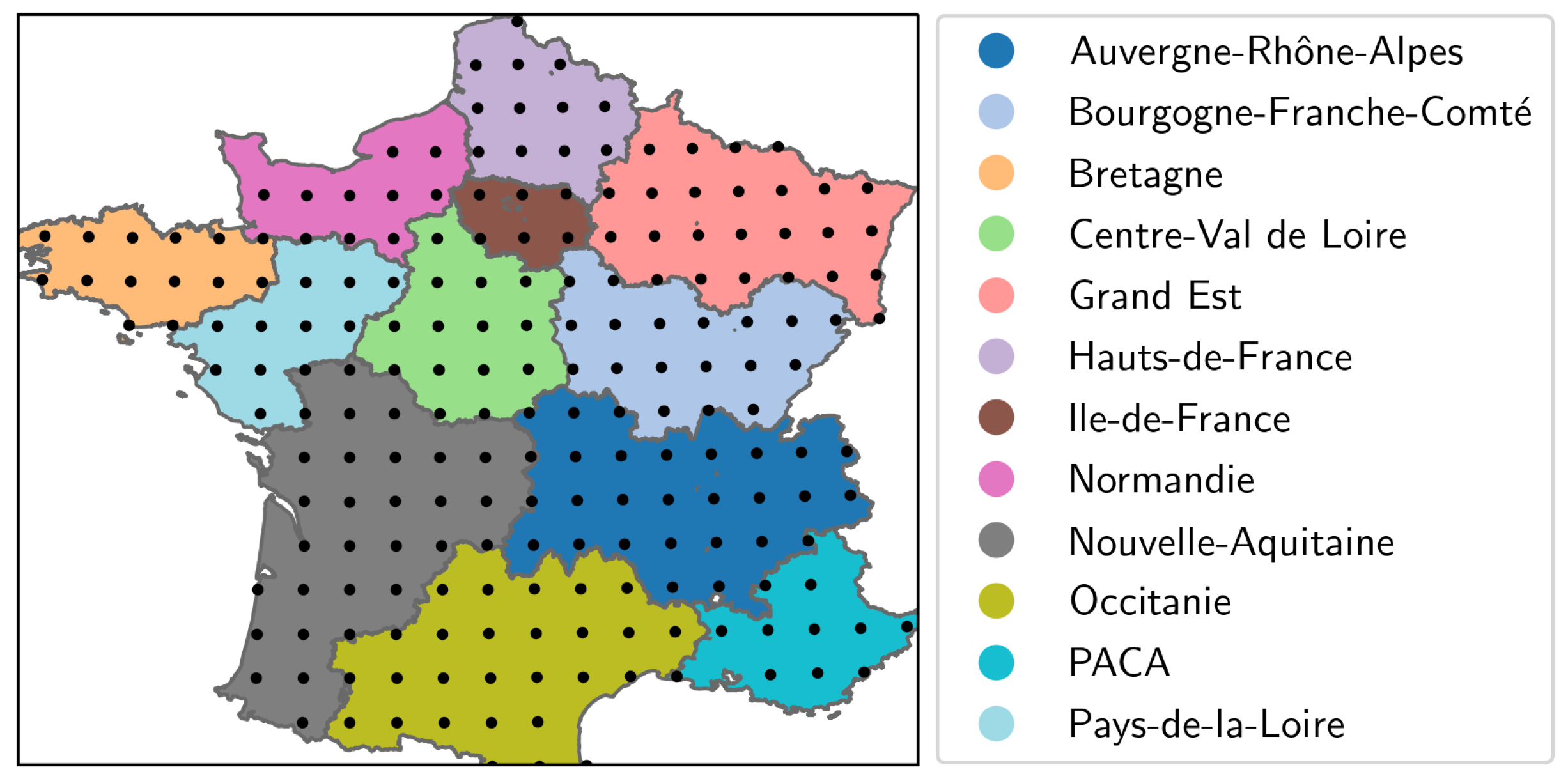
We ask what are the adequacy costs arising from the variability of the renewable-energy production in France depending on the dispatch variable costs and investigate the role of geographical and technological diversification [32] (for an overview of renewable energies in France in 2020). Empirical data are used to apply the cost minimization problems described in the previous Section 2 to the French electricity system. More specifically, the optimization problem with quadratic dispatch costs (Section 2.5) is applied to the case of onshore wind and PV energy in metropolitan France. Each pair of VRE technology and administrative region is associated to a VRE producer in the model. The domain, the national load, the regional CFs per technology and the rental costs need first to be defined.

3.1. Domain

The domain is divided in the 12 administrative regions of metropolitan France (to define the geometry of the regions, shapefiles from https://www.data.gouv.fr, accessed on 1 June 2021 are used), as shown in Figure 2. This gives $12\times 2=24$ VRE producers for the two VRE technologies considered here.

3.2. Load and CF Time Series

Following Tantet et al. [23], regional VRE CF time series from 2010 to 2019 (10 y) are estimated at an hourly sampling from the climate data provided by the MERRA-2 reanalysis. This is done per grid point of the climate data, with each grid point being associated to a region, as illustrated in Figure 2. The result is averaged per region and adjusted using a Ridge linear regression with cross-validation to CF data from 2014 to 2019 (6 y) provided by the French transmission system operator, RTE (https://opendata.reseaux-energies.fr/explore/dataset/fc-tc-regionaux-mensuels-eolien-solaire/information/?disjunctive.region, accessed on 1 June 2021). The averages of the regional CFs ($\langle H_i\rangle$) are represented in Figure 3a,b.

Similarly, the thermosensitive demand model developed by Tantet et al. [23] is used to estimate national demand time series computed from the MERRA-2 temperature data and fitted against the demand data from RTE (https://opendata.reseaux-energies.fr/explore/dataset/eco2mix-regional-cons-def/information/?disjunctive.libelle_region&disjunctive.nature, accessed on 1 June 2021). These estimations are perfomed using the e4clim modeling platform [33] introduced by Tantet et al. [23].

3.3. Rental Costs

The yearly rental costs for onshore wind and PV ($T_0{\mathrm{hRC}}_i$) are computed by summing the annualized capital costs (annuity) and the fixed O&M costs. They are given in

Table 1. Costs and lifetimes used to compute the yearly rental costs for the variable renewable energy technologies (data from Tsiropoulos et al. [29]).

	Units	Onshore Wind	Photovoltaic
Overnight Cost	€/kWe	1.13 × 103	423
Lifetime	y	25	25
Annuity	€/kWe/y	81.2	30.7
Fixed O&M Cost	€/kWe/y	34.5	9.20
Yearly Rental Cost	€/kWe/y	116	39.9

. The annualized capital cost, ${\left(\mathrm{Annuity}\right)}_i$, for some technology i, is computed according to [16].

$$\begin{array}{c}\hfill {\left(\mathrm{Annuity}\right)}_i=\frac{\rho {\left(\mathrm{Overnight}\mathrm{Cost}\right)}_i\left(\rho {\tau }_c+1\right)}{1-{\left(1+\rho \right)}^{-{\left(\mathrm{Lifetime}\right)}_i}},\end{array}$$

(24)

where ${\tau }_c$ is a construction time fixed to 1 y and $\rho$ is a discount rate fixed to $4.5\%$, as recommended by the French government for use in public socio-economic analyses [34]. This choice of a discount rate value defined for socioeconomic evaluations of public investments has two motivations. First, we aim at keeping the cost definition as simple as possible by selecting a single discount rate for the VRE sector, ignoring the specificities of individual projects. Second, considering the large investments in VRE capacities considered here, we set this work in the framework of a long-term socioeconomic strategy, whereby investment choices by decentralized actors are guided by the public power. We thus prefer to rely on a discount rate that takes systemic risk into account rather than to rely on a discount rate coming from energy markets ignoring several externalities.

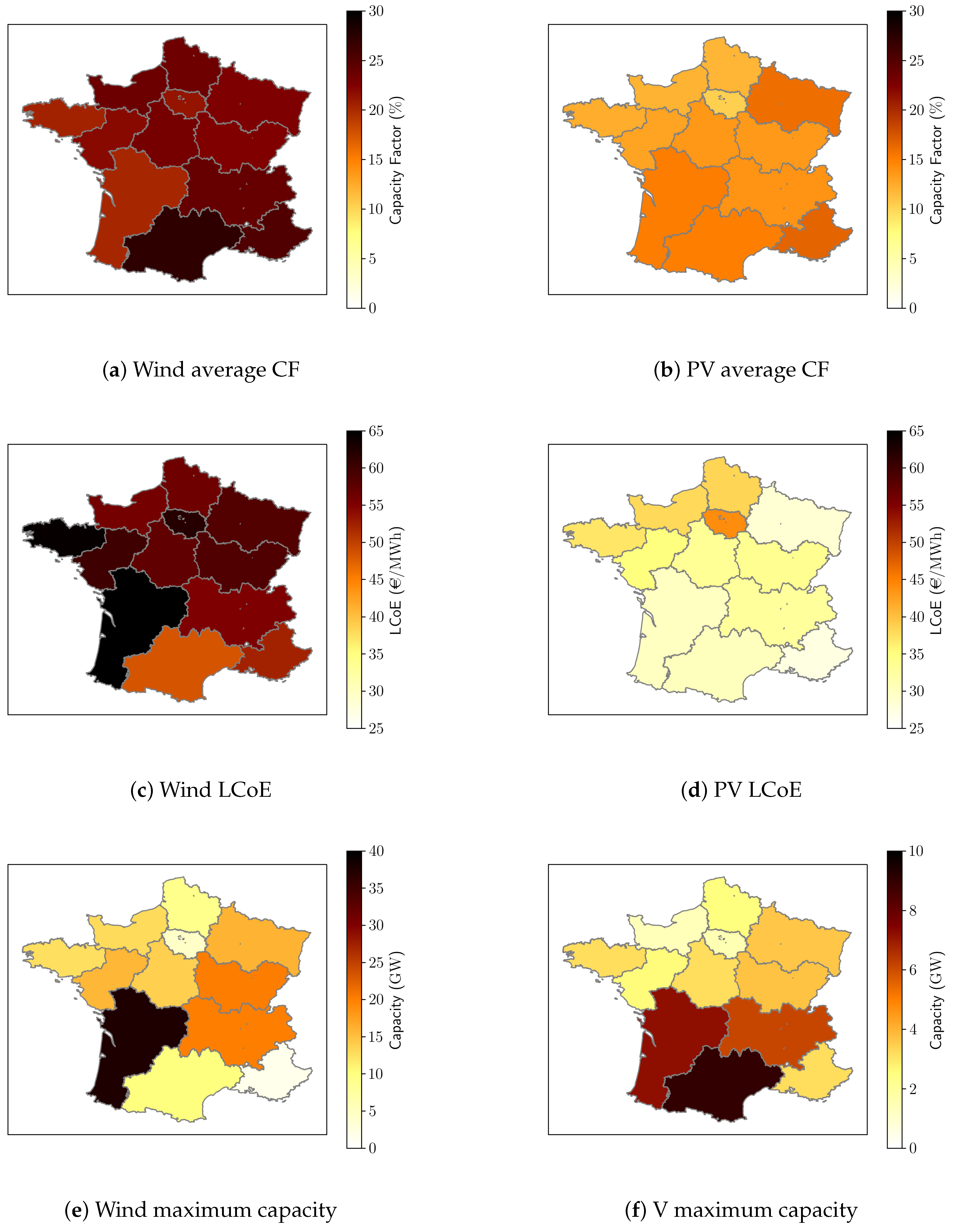
3.4. Levelized Costs of Electricity

The VRE LCoEs (${\mathrm{LCoE}}_i$) is computed applying Equation (8) using the rental costs from Table 1 and the average CFs represented in Figure 3a,b. The resulting LCoEs are represented in Figure 3c,d.

3.5. Maximum Dispatchable and VRE Capacities

The total dispatchable capacity ($x_{\mathrm{Di}}$) is fixed to the maximum over the period of the one-hour load, which is about 107 GW, so that the load can always be met by the dispatchable generation alone. (The following information is not used here, but helps put the abstract results from this study in perspective with the actual electricity system. In 2018, the installed capacities per technology were 19 GW for fossil thermal, 26 GW for hydropower and 63 GW for nuclear, while other renewable sources were totaling about 3 GW. Nuclear, fossil thermal and hydropower capacities were thus totaling about 107 GW. However, there was a net export of 60 TWh corresponding to a capacity at full CF of 60.2 × 10³/8760 = 6.87 GW.) The data is taken from https://opendata.reseaux-energies.fr/explore/dataset/parc-prod-par-filiere/information/ (accessed on 1 June 2021) and https://opendata.reseaux-energies.fr/explore/dataset/imports-exports-commerciaux/information/ (accessed on 1 June 2021). The maximum regional VRE capacities ($x_i^{\max }$) are taken from ADEME [35] and are represented in Figure 3e,f. These values are for industrial-scale onshore wind and PV installations. They exclude rooftop residential PV.

3.6. Solver

The optimization problems are solved using the Pyomo [36,37] interface to the Ipopt algorithm [38]. For a given value of $\alpha$, a numerical approximation of the optimal solution is found in a few minutes on a computer with an Intel Core i7 processor of the 8th generation (8 cores) and with 32 Gb of random access memory. This optimization module is integrated to the new version of the e4clim modeling platform [33]. The problem is solved independently for different values of $\alpha$ ranging from 1.0 × 10⁻⁶ to 6.0 × 10⁻³ with a step of 1.0 × 10⁻⁴ €/MWh². The robustness to sampling is tested in Appendix C by comparing numerical results obtained from load and CF time series of increasing duration estimated from the MERRA-2 data. The choice of using only 10 years of data is found to lead to differences of only a few percents compared to using 5, 15, or 20 years and does not affect the conclusions of this study.

4. Results

Before discussing the role of variability in the model, the variable problem optimal solutions are first analyzed.

4.1. Variable-Problem Behavior

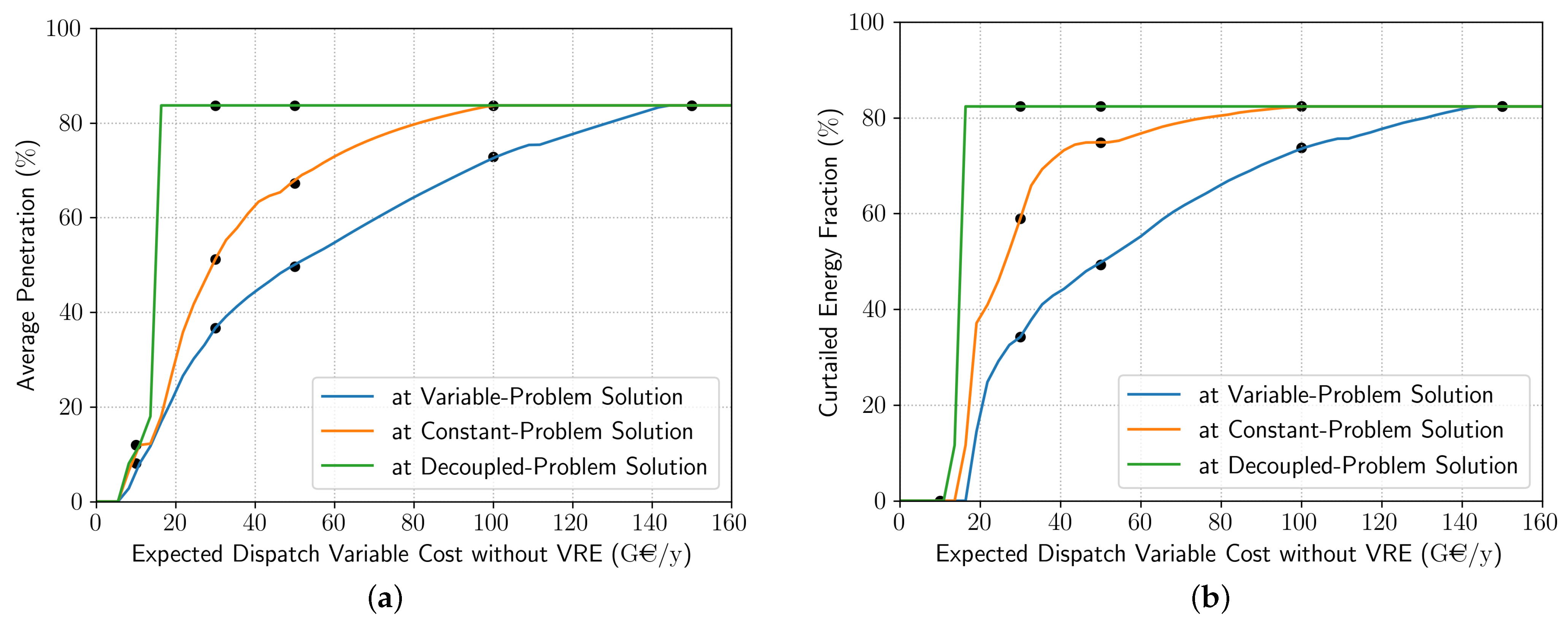
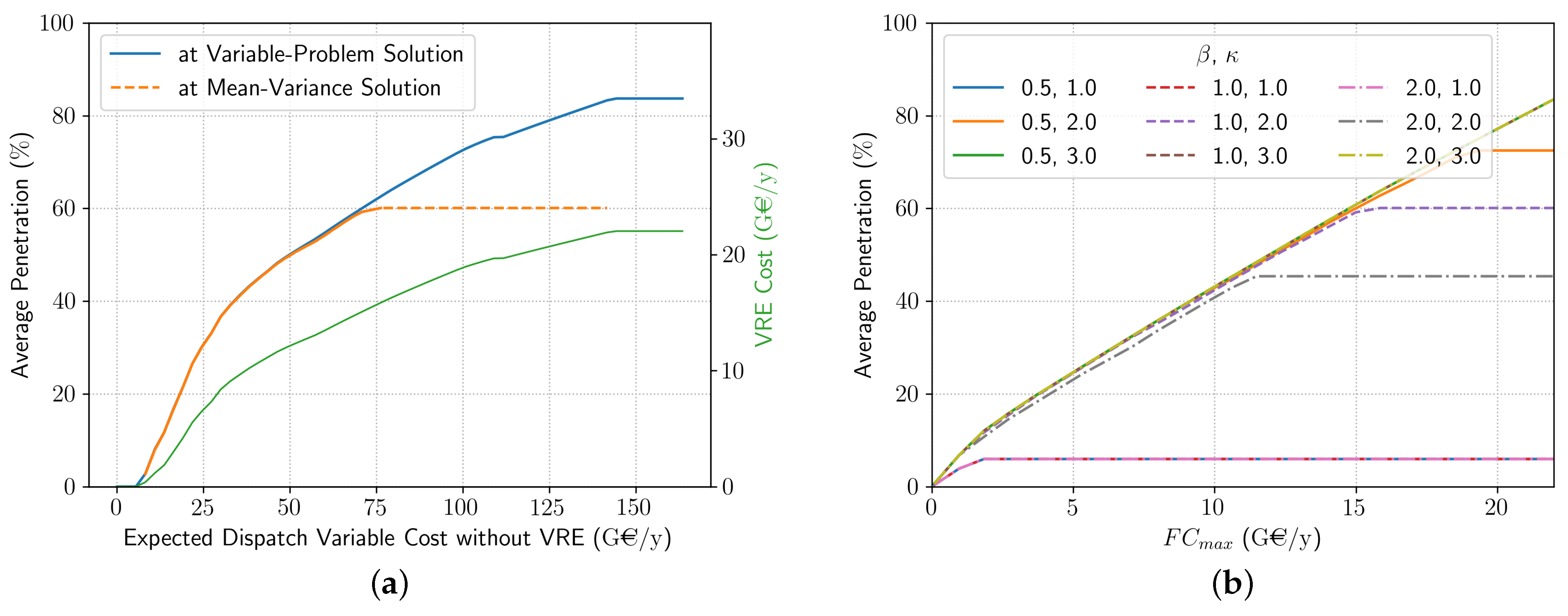
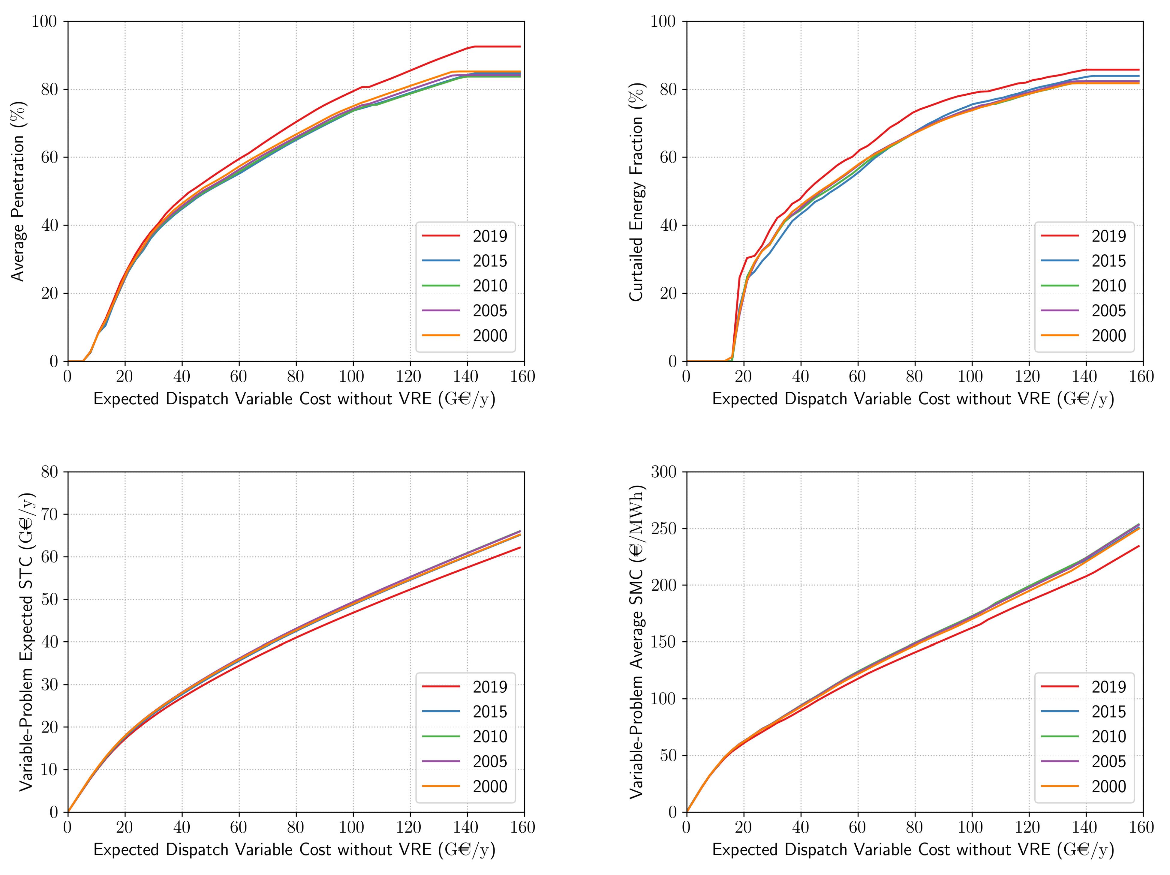
4.1.1. Average Penetration

The average VRE penetrations for numerical approximations of the optimal solutions to the variable problem (Equation (4)) are represented by the blue line in Figure 4a, as a function of $\alpha$. To ease the interpretation of the figure, however, $\alpha$ in abscissa is replaced by the STC without VRE, i.e., the expected dispatch variable cost $\mathbb{E}\left(\overline{\mathrm{STC}}\left(0\right)\right)=T_0\langle \alpha L^2\rangle$ for the French national load. The penetration increases quickly with the variable cost of the dispatchable generation, but stabilizes around 84%. This increase is expected from the fact that the VRE cost (which is not affected by $\alpha$) decreases relatively to the dispatch variable cost. A direct consequence is the decrease in the utilization of the dispatchable production.

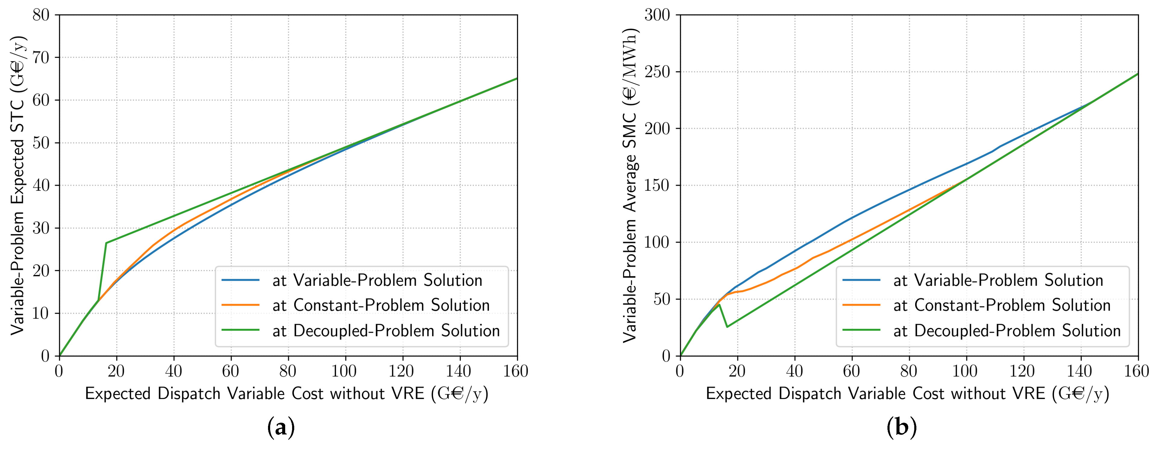
4.1.2. System Costs and Wholesale Price Effect

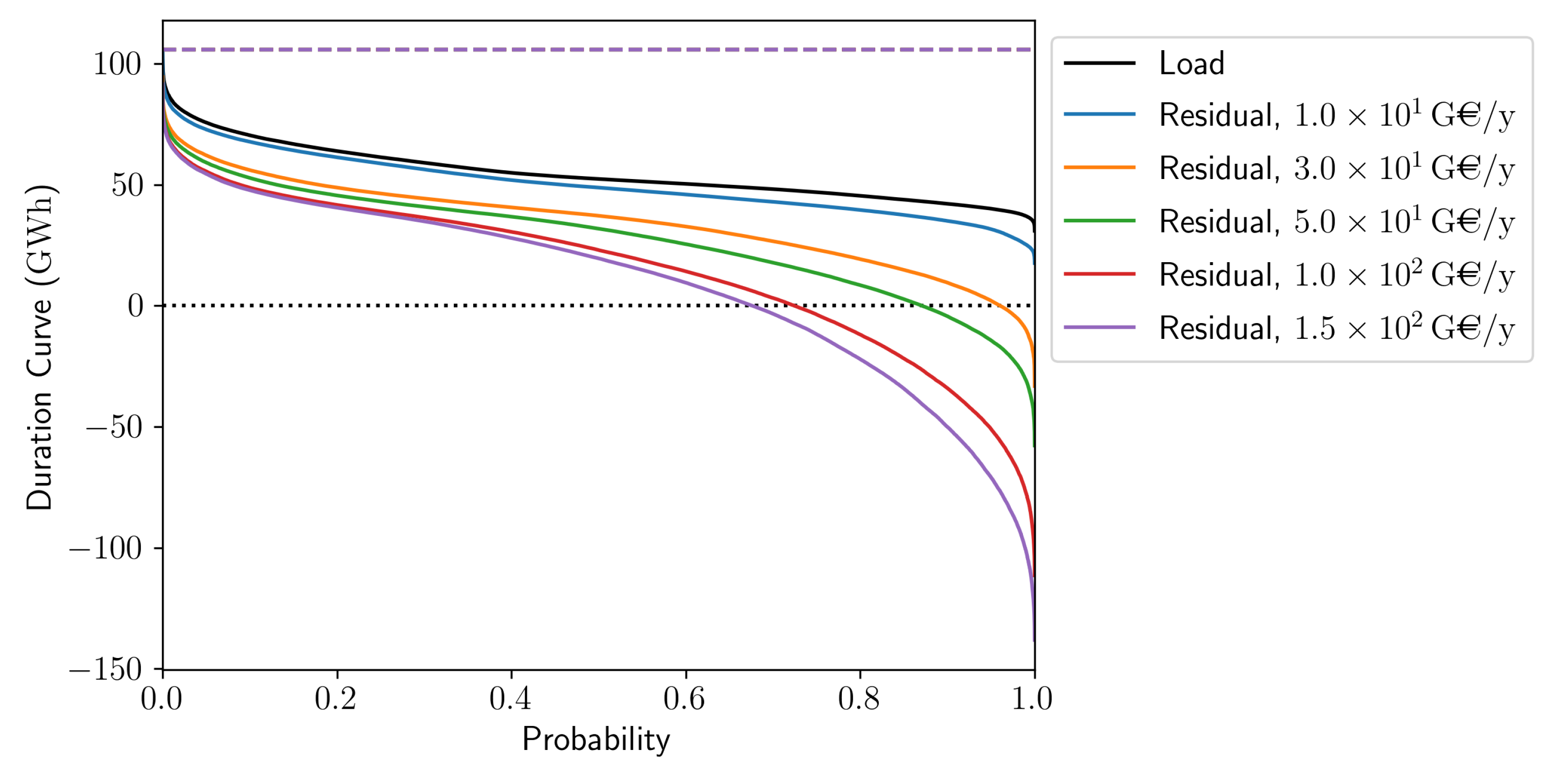
The average SMC and the expected STC for optimal solutions of the variable problem are represented by the blue line in Figure 5a,b, respectively. Overall, the STC and the SMC with VRE increase with the dispatch variable cost. However, this growth is not linear but is instead mitigated by the introduction of VRE capacities, as further discussed in Section 4.3.

4.1.3. Curtailment

Next, one can see from Figure 4b that for penetrations larger than approximately 10%, curtailment of the VRE production occurs. The fraction of energy curtailed quickly increases with the penetration. One can observe from the Residual Load Duration Curve (RLDC), represented in Figure 6, that both the amount of energy curtailed at individual hours and the frequency at which curtailment occurs increase with $\alpha$. At large penetrations, the maximum amount of energy curtailed is actually comparable to the maximum load. Thus, the absence of storage, demand-side management or additional dispatchable renewable capacities—together with the high variability of the total VRE generation when restricted to France—results in large amounts of renewable energy being curtailed even at moderate penetrations.

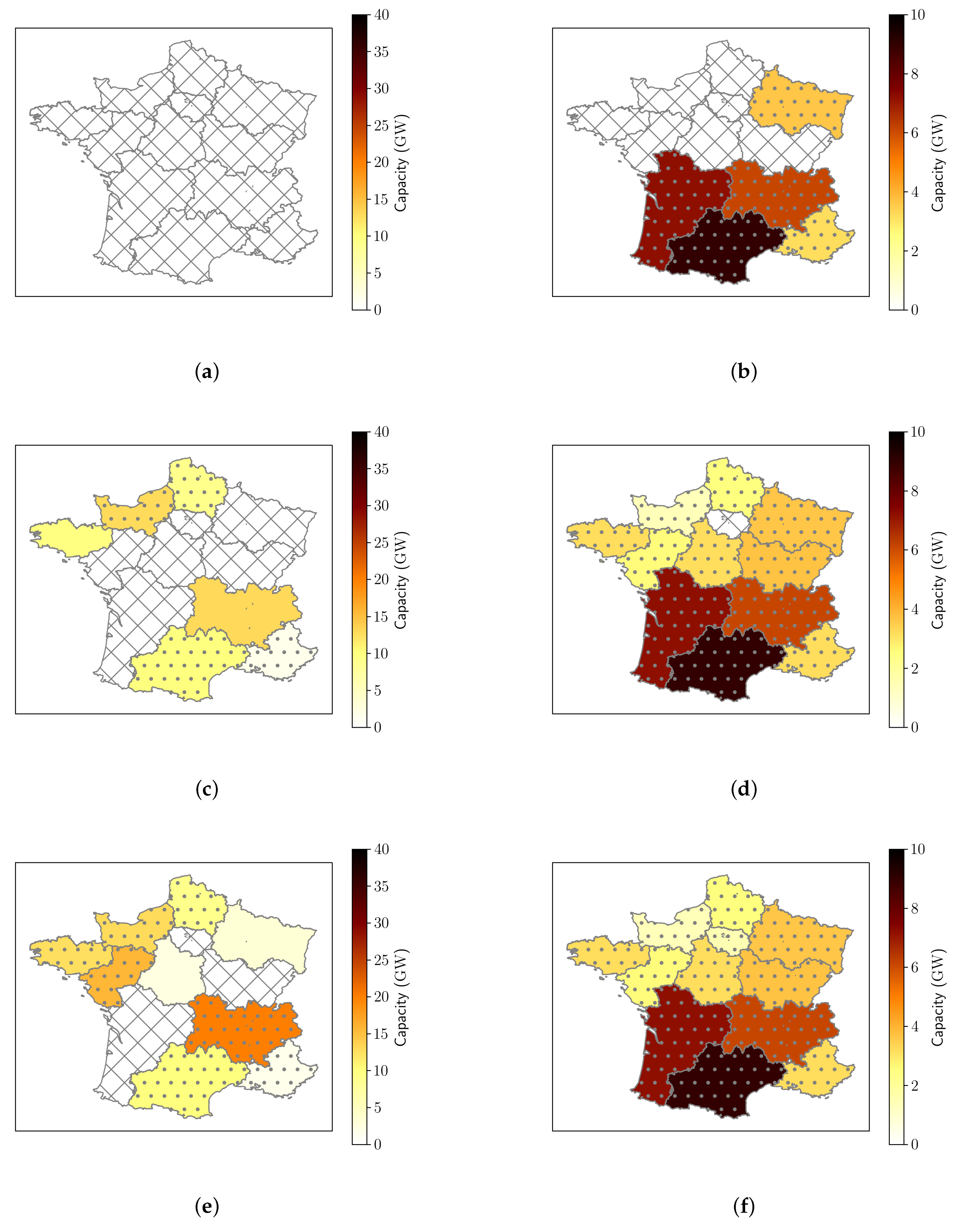
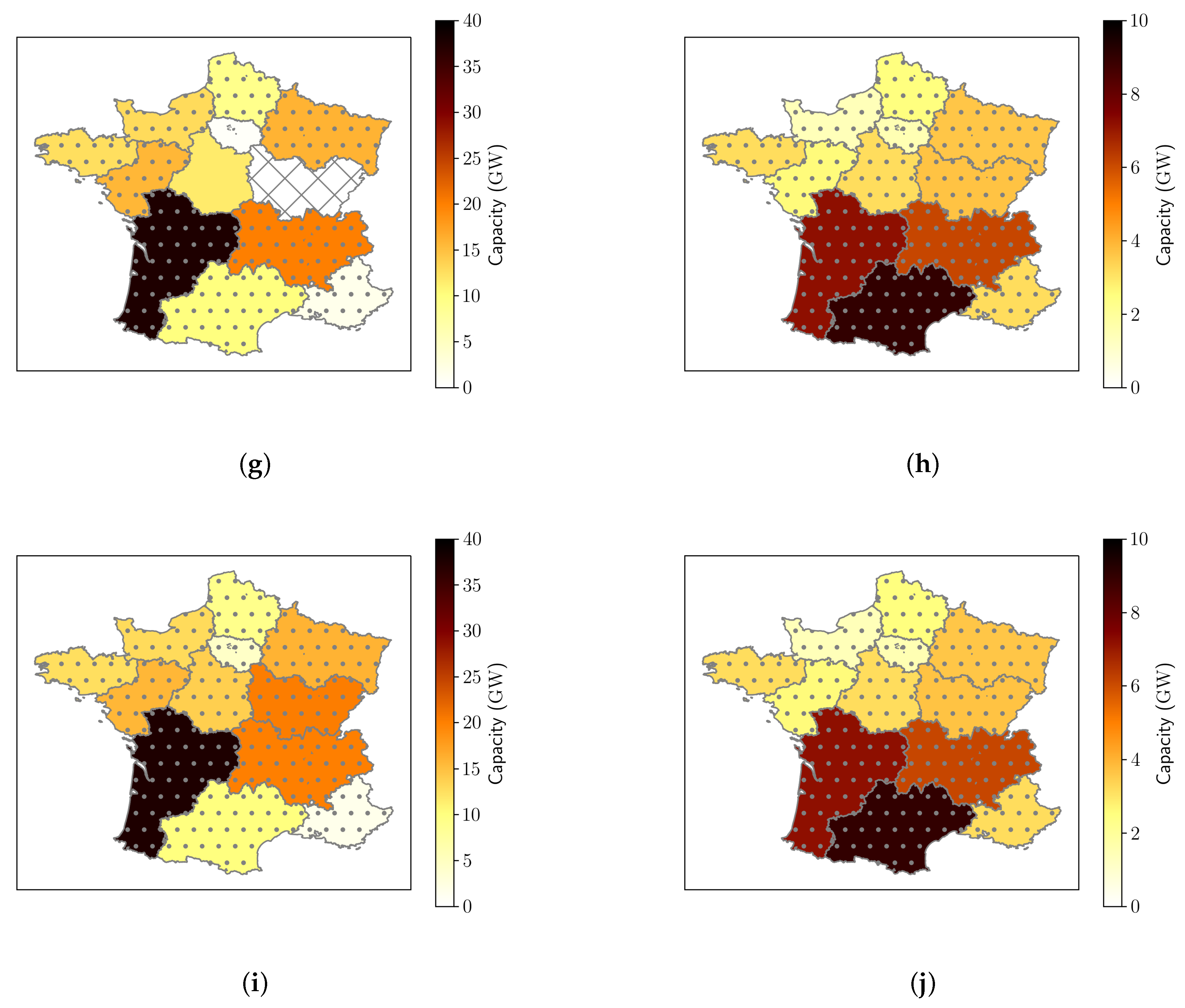
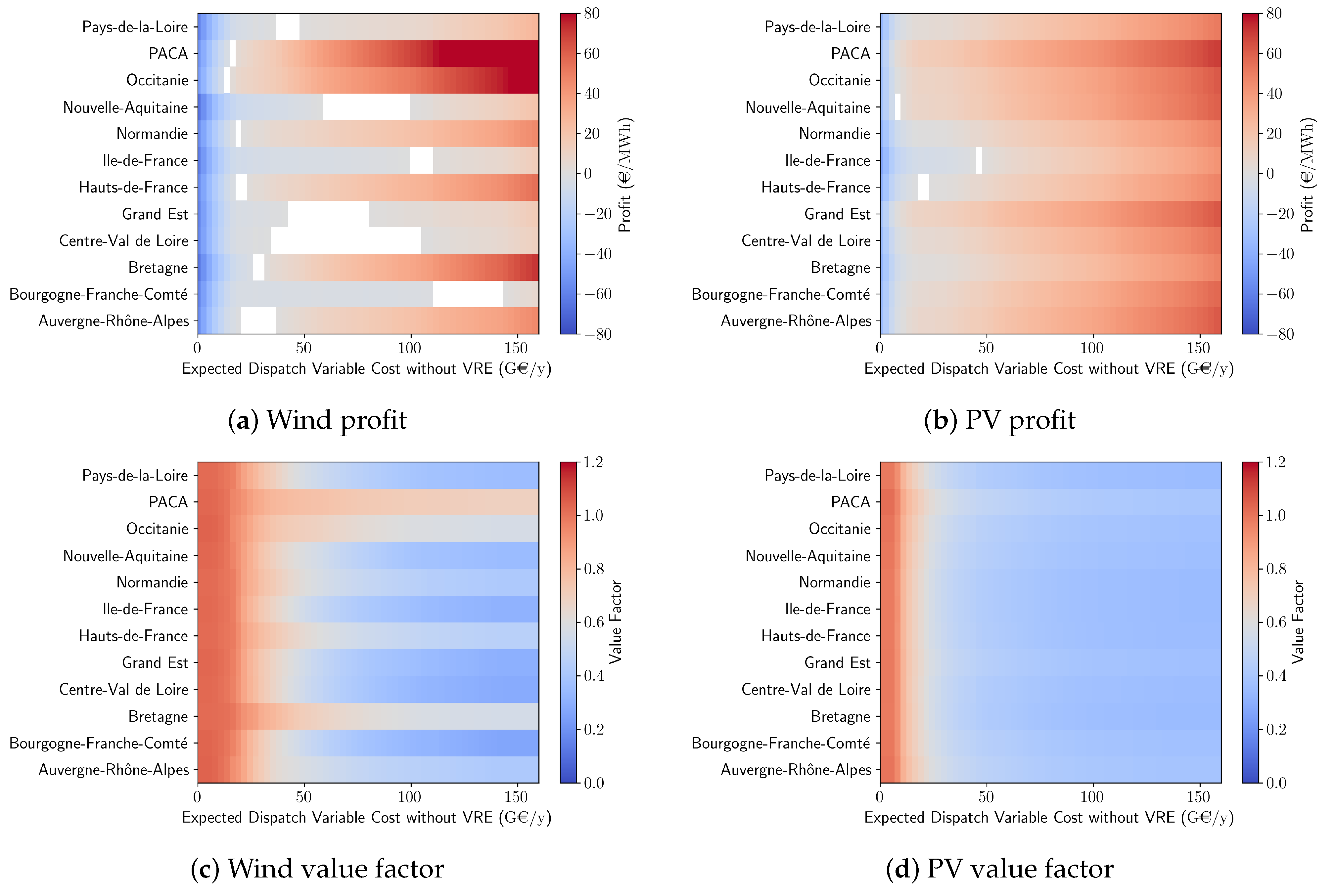
4.1.4. VRE Regional Capacities and Profits

A more detailed picture of the optimal solutions emerges from the regional distributions of the optimal VRE capacities represented in Figure 7. In addition, Figure 8 helps relate the installed capacities to the profits and value factors of the corresponding VRE producers. One can observe that, as $\alpha$ is increased, VRE profits and capacities tend to increase although the increase in the average SMC (Figure 5b) is partially compensated by the decrease in the value factors.

More specifically, one can see that PV capacities in the south and in the east are first installed (Figure 7a,b). In these regions, PV is installed up to maximum capacity so that no two technology regions have positive capacities smaller than their maximum capacity. This behavior is consistent with an economic analysis based on the LCoE and accounting for the impact of the VRE generation on the SMC, as encoded in the constant problem. One can see from Figure 3c,d that the LCoE is indeed smaller for PV than wind (due to the smaller rental cost of PV, see Table 1), and for PV in the south and in the east compared to other regions (due to the higher average CFs in these regions, see Figure 3b). In fact, for such low values of the expected STC without VRE, the PV value factors for the variable problem are all close to one (Figure 8d), so that the PV profits are indeed maximal for these regions (Figure 8b). The profits for these regions are in fact positive, which indicates that an economic rent is generated because of the capacity limits in these regions.

For higher expected STC withtout VRE values (Figure 7c–j) wind capacities are installed in addition to more PV capacity. In Figure 7c,e, one can see that two wind regions are positive without reaching their maximum capacity. This shows that optimal solutions deviate from the constant problem and that correlations between technology regions play an important role (see Section 2.3). This is confirmed by the fact that the wind profits for these regions remain zero around the corresponding values of the expected STC without VRE (Figure 8a). This indicates that the increase in the SMC with $\alpha$ is exactly compensated by the decrease in the wind value factors of these regions (Figure 8c).

4.1.5. Economic Rent at High Penetrations

For an expected STC without VRE of 150 G€/y, all technology regions have reached their maximum capacity (Figure 7j). This explains why the optimal solutions remain constant for values of the expected STC without VRE larger than about 140 G€/y. The maximum capacity constraints prevent installing more VRE capacities even though this would further reduce the STC. As a result, the average penetration cannot be larger than about 84%. This results in positive VRE profits (Figure 8a,b) due to economic rents, as discussed in Section 4.3.

4.2. Optimizing Ignoring the Wholesale Price Effect and Variability

The impact of the residual load variability on optimal mixes depending on $\alpha$ is now investigated.

First, optimal solutions for the variable, constant, and decoupled problems are compared. Their properties are respectively represented by blue, orange, and green lines in Figure 4 and Figure 5. For the decoupled problem, VRE penetration increases sharply with the expected STC without VRE and reaches its maximum value quickly, as expected from the absence of merit-order effect reducing the SMC. In this case, VRE capacity for a technology-region is installed up to maximum capacity as soon as the decoupled SMC (Equation (12)) is larger than the corresponding LCoE (Section 2.3.1).

In all these plots, the constant-problem solutions (in orange) lie between the decoupled- and the variable-problem solutions. This shows that taking the merit-order effect into account limits the installation of VRE capacities because the resulting SMC remains smaller than in the decoupled problem, but that ignoring variability leads to installing more VRE than otherwise.

Due to the higher penetrations of the decoupled- and constant-problem solutions, the SMC is smaller than for the variable-problem solutions for intermediate values of the penetration (Figure 5b). It thus appears that the cost of electricity is cheaper for optimal mixes ignoring the merit-order effect and/or variability. However, the drawback is that the resulting expected STC is larger (Figure 5a) so that the decoupled and constant mixes are sub-optimal when taking VRE rental costs into account. At high penetrations, these differences are small because the solutions of all three problems converge to the maximum capacity distributions. For moderate values of the expected STC without VRE, however, the differences in expected STC between the decoupled- and variable-problem solutions can be more than twice as high. On the other hand, the expected STC for constant-problem solutions is only a few percent higher than for the variable-problem solutions. This shows that the cheaper SMC is more than compensated by higher expenditures from investing in more VRE capacities, but not so much so.

Thus, while ignoring the merit-order effect when optimizing investment in VRE capacities may lead to significant sub-optimality, ignoring variability appears to be less of an issue in this simple model and for the French configuration analyzed here.

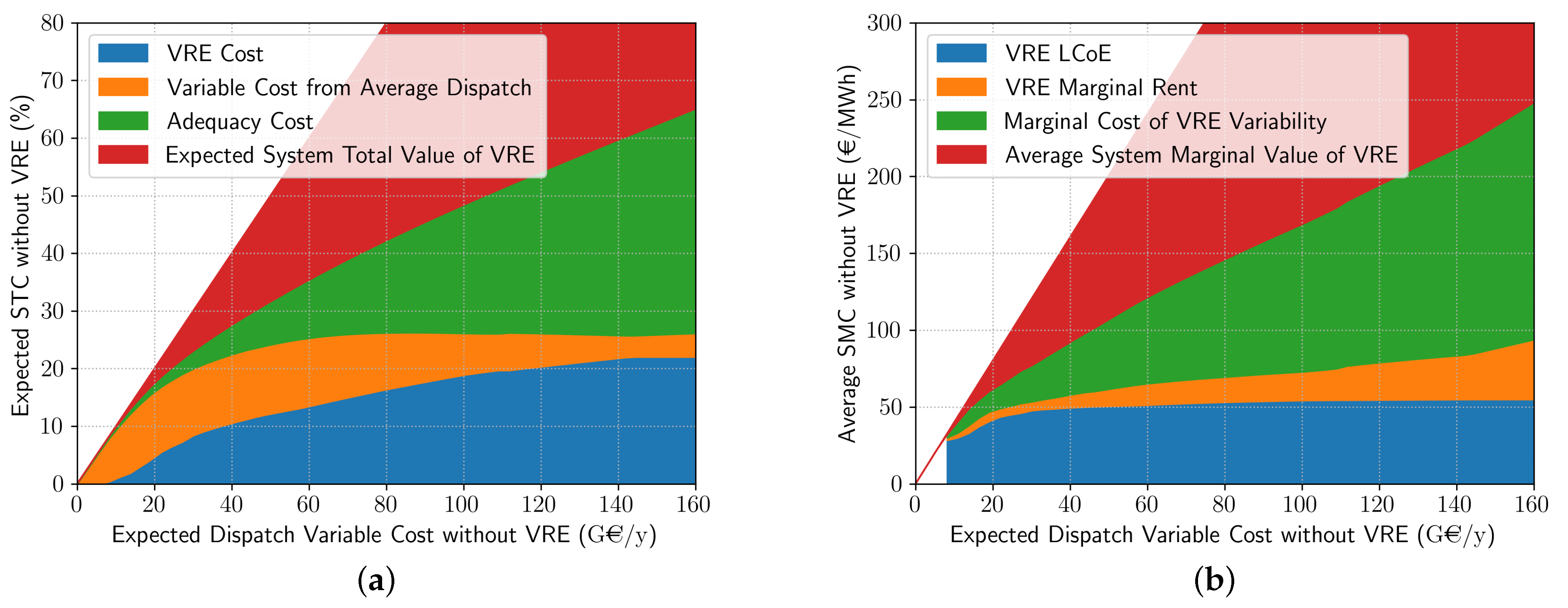
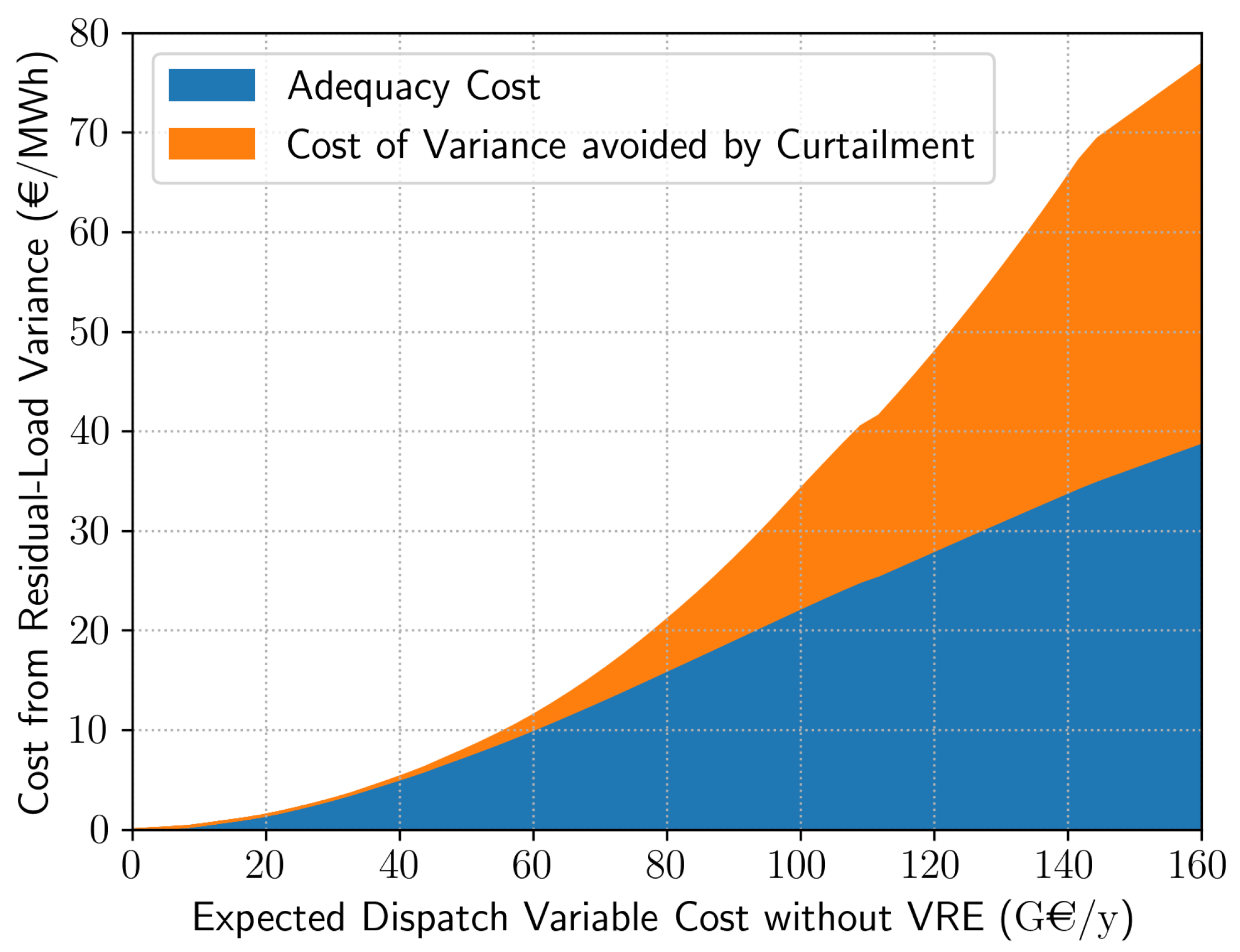
4.3. System Value of VRE and Adequacy Cost

The system total and marginal value of VRE are now analyzed. They are represented by the red area in Figure 9. They are always positive and both increase sharply with the expected STC without VRE, which explains the increase in the average VRE penetration (Figure 4a). This increase is associated with a relative decrease of the dispatch variable cost of the average residual load (orange area compared to the top red line in Figure 9a). However, dispatchable generation is still needed, even at large penetrations, and is responsible for a large fraction of the STC and of the SMC (green area in Figure 9a,b, respectively). At high penetrations, the adequacy cost actually dominates the fixed cost of VRE, and the marginal cost of variability is larger than both the LCoE and the marginal rent, even though the latter increases as more VRE technology-regions reach their maximum capacity.

The average system marginal value (in red, Figure 9b) is given by the difference between the decoupled and the variable versions of the average SMC. Its increase is thus a manifestation of the wholesale price effect which is responsible for a reduction of the SMC only partially compensated by the marginal cost of VRE variability. In addition, the difference between the constant and the variable versions of the expected STC (in green, Figure 9a) gives the adequacy cost. At zero VRE penetration, these adequacy costs are due to the variability of the load only and represent 3.8% of the expected STC. They quickly increase with the VRE penetration to reach 58% of the expected STC at the smallest value of $\alpha$ at which the maximum penetration is reached. This confirms that the nonlinearity of the dispatch variable cost function leads to large adequacy costs that should not be ignored for significant VRE penetrations.

Finally, Figure 10 represents the decomposition of the adequacy costs in a variance term and a curtailment term, according to Equation (17). It shows that the adequacy costs would actually be much larger (up to 100%) if the excess VRE generation had to be absorbed at the cost of the dispatchable generation instead of being curtailed.

To conclude, while differences in the resulting costs of the optimal variable, constant and decoupled mixes may not be so strong when ignoring the wholesale price effect and variability in the optimization (Section 4.2), differences in the variable, constant, and decoupled versions of the expected costs are significant. This means that planning a budget ignoring adequacy costs and the wholesale price effect leads to underestimating the STC and overestimating the SMC, respectively.

5. Comparison with Mean-Variance Analyses

In order to relate different optimization approaches to the problem of renewable energy integration, we now identify a special case of the cost-minimization problem (Equation (4)) to a particular form of mean-variance analysis.

5.1. Cost Minimization without Curtailment

In the absence of curtailment, the dispatchable generation for the optimal schedule (Equation (5)) is given by the residual load. The variable problem (Equation (4)) then turns into a single-stage long-term investment problem with only the VRE-capacity distribution ($\mathit{x}$) as decision variable. With quadratic dispatch costs (Equation (23)), the STC divided by $T_0$ becomes

$$\begin{array}{c}\hfill \alpha {\langle L-Q_{\mathit{x}}\rangle }^2+\alpha \mathrm{Var}\left(L-Q_{\mathit{x}}\right)+\sum _{i=0}^{m-1}{\mathrm{hRC}}_i{x}_i,\end{array}$$

(25)

where $\mathrm{Var}\left(X\right)=\langle {(X\left(t\right)-\langle X\rangle )}^2\rangle$ is the variance both in time and over samples of some process X. We refer to it simply as the variance of X. In this case, the STC is decomposed in an average term, a variance term, and a third term for the VRE rental cost. The first term is minimized by increasing the VRE penetration

$$\begin{array}{c}\hfill {\mu }_{\mathit{x}}=\frac{\langle Q_{\mathit{x}}\rangle }{\langle L\rangle },\end{array}$$

(26)

to 100%. The variance of the residual should also be controlled. The variance of the load being fixed, this can be done by adjusting capacities so as to increase the covariance between the VRE production and the load and/or to limit the variance of the total VRE production. This is in turn achieved via the diversification of the VRE mix and by favoring technology regions for which the VRE CFs are more correlated to the load. In the presence of curtailment, the optimization problem is more difficult to interpret, in particular because curtailment limits the variance of the dispatchable generation compared to the variance of the residual load.

5.2. Differences in Formulation with Some Mean-Variance Applications to VRE Systems

Table 2. Summary of the defining elements of Markowitz’ original portfolio theory and of some mean-variance analysis applications to the energy sector.

Reference	State	Mean of	Variance of	Total Constraint
Markowitz [17]	Relative amount invested	Return	Return	100% invested
Beltran [19]	Capacity fraction	Generation cost	Generation cost	100% installed
Thomaidis et al. [21]	Capacity fraction	Generation	Generation	100% installed
Santos-Alamillos et al. [22]	Capacity fraction	Generation	Generation	100% installed + bounds on capacity
Tantet et al. [23]	Capacity	Generation/load	Generation/load	Total capacity
Bouramdane et al. [24]	Capacity	Generation/load	Generation/load	VRE fixed cost
This study	Capacity	Squared mean net-load	Net load	VRE fixed cost

summarizes the design of some mean-variance analysis problems applied to the VRE systems [19,21,22,23,24].

The formulation of the mean-variance problems in these studies differ from the cost-minization problem (Equation (4)) and its version ignoring curtailment (Equation (25)) in several aspects:

• No curtailment of the residual load is performed in the mean-variance case.
• VRE rental costs are not included in the objective functions, but the (fractional) total capacity or rental cost is instead constrained. Apart from Beltran [19], who use generation costs in the mean and variance terms, and Bouramdane et al. [24], who use a total rental cost constraint, no economic costs appear in most mean-variance problems.
• As opposed to the mean-variance problems listed here, the mean of the residual load is squared in the cost minimization problem (Equation (25)).
• In the mean-variance problems, a coefficient weighs the objective for the variance with respect to the objective for the mean. In the cost minimization problem, $\alpha$ instead weighs the mean of the squared residual (mean squared plus variance) with respect to the VRE rental cost.

5.3. A Formulation of Mean-Variance Analysis Akin to Cost Minimization

To remain close to the cost minimization problem (Equation (25)), one possible formulation of the cost function of the mean-variance problem takes the form

$$\begin{array}{c}\hfill {\langle L-Q_{\mathit{x}}\rangle }^{\kappa }+\beta \mathrm{Var}\left(L-Q_{\mathit{x}}\right),\end{array}$$

(27)

subject to the usual constraint that VRE capacities should be positive and to a constraint on the VRE rental cost,

$$\begin{array}{c}\hfill \sum _{i=0}^{m-1}{\mathrm{hRC}}_i{x}_i\le {\mathrm{FC}}_{\mathrm{tot}},\end{array}$$

where ${\mathrm{FC}}_{\mathrm{tot}}$ is the bound on the total VRE cost. The positive coefficient $\beta$ is used to scalarize the bi-objective mean-variance optimization and controls the weight of the variance term with respect to the mean term. The exponent $\kappa$ is usually set to one, but setting $\kappa$ to 2 has the advantage of leaving the solutions to the optimization problem unchanged when scaling the residual load. The corresponding Lagrangian, living aside the positivity bounds, is

$$\begin{array}{c}\hfill {\langle L-Q_{\mathit{x}}\rangle }^{\kappa }+\beta \mathrm{Var}\left(L-Q_{\mathit{x}}\right)+\gamma \left(\sum _{i=0}^{m-1}{\mathrm{hRC}}_i{x}_i-{\mathrm{FC}}_{\mathrm{tot}}\right),\end{array}$$

(28)

where the non-negative coefficient $\gamma$ is the KKT multiplier for the VRE rental cost constraint.

The Lagrangian of Equation (28) and the cost function of Equation (25) are now compared, keeping in mind that the latter is a valid formulation of the cost function of the variable problem only in the absence of curtailment. Note first that, given some values of $\kappa$ and $\beta$, there exists a threshold for ${\mathrm{FC}}_{\mathrm{tot}}$ below which the VRE rental cost constraint of the mean-variance problem is active. Then, for ${\mathrm{FC}}_{\mathrm{tot}}$ below this threshold and for $\kappa =2$ and $\beta =1$, the mean-variance problem is equivalent to the cost minimization problem. By this we mean that, given ${\mathrm{FC}}_{\mathrm{tot}}$, there is a unique value of $\alpha$ for which the optimal solution to the mean-variance problem (Equation (27)) is also a solution to the variable problem (Equation (25)), and vice versa. Beyond this threshold, the VRE rental cost constraint is inactive and further increasing ${\mathrm{FC}}_{\mathrm{tot}}$ has no effect on the optimal solution of the mean-variance problem.

This result is illustrated in Figure 11a for the case of France studied in Section 3. The average penetration is represented versus the expected STC without VRE for numerical approximations of the optimal solutions to the variable problem and to the mean-variance problem. Because an optimal solution to the mean-variance problem does not depend on $\alpha$, this representation is made possible by assigning to such a solution the value of the variable cost of the dispatchable generation of the optimal solution to the variable problem with a VRE rental cost (represented by a thin green line one the right y-axis) equal to the maximum VRE rental cost defining the mean-variance problem (${\mathrm{FC}}_{\mathrm{tot}}$). One can see that, for low values of the variable cost of the dispatchable generation, the optimal solutions to both problems are relatively close to each other. Small differences are explained by the presence of curtailment in the variable problem which is ignored in the mean-variance problem. For values of the variable cost of the dispatchable generation larger than about 70 G€/y, however, solutions diverge. This happens when the VRE rental cost constraint of the mean-variance problem is inactive. Optimal solutions to this problem are no longer constrained because it is the stronger increase in the variance of the residual load than in its mean that limits the increase in VRE capacities. This behavior is limited in the cost-minimization problem because the effect of curtailment on the cost is taken into account.

In addition, one can see in Figure 11b comparing the average penetration of the optimal solutions to the mean-variance problem for different values of $\kappa$ and $\beta$ that these solutions are highly sensitive to the choice of the parameters. In conclusion, while it is possible to define a mean-variance problem that is close to a STC-minimization problem, solutions to both problems diverge significantly in the presence of curtailment and if the parameters of the mean-variance problem are not chosen properly.

6. Summary and Discussion

We develop a simple model of VRE integration at high penetrations that

• considers both the problem of long-term investment in VRE capacities and the optimal schedule of the dispatchable generation to satisfy an increasingly variable net load;
• minimizes the STC in order to include adequacy costs and estimate the system value of VRE; and
• avoids modeling the full system of dispatchable units by treating them as a fully-dispatchable aggregate.

This last point is a strong approximation, but provides a minimal model of optimal VRE investment allowing one to estimate and decompose the VRE system value by capturing the average effect of VRE integration on the wholesale price as well the impact of VRE variability.

Assuming that the dispatch variable costs are quadratic leads to the simplest version of the model. We show that this version is identical to a mean-variance problem, but that the absence of curtailment and the proper choice of parameters are critical for this to be the case.

We apply this version to the case of France over the 2010–2020 period with limited PV and wind capacities distributed over the twelve administrative regions of metropolitan France. Larger dispatch variable costs obviously lead to higher optimal VRE penetration cost but with significant amounts of energy being curtailed and with the limitation imposed by maximal VRE capacities. We show that while ignoring the wholesale price effect and variability has a relatively small impact on the optimal investment, differences in the expected VRE value are significant. This means that planning a budget ignoring adequacy costs and the wholesale price effect leads to underestimating the STC and overestimating the SMC, respectively.

A key advantage of this model is that the numerical estimation of its optimal solutions using a sample-average approximation is relatively fast and that optimal solutions can quickly be tracked depending on the parameterization of the dispatch variable cost in response, for instance, to a carbon price. In addition, the system total and marginal values of VRE can easily be computed. This makes the model presented here useful to study the impact of the integration of high shares of VREs in an electricity system. This comes of course at the price of a crude modeling of the conventional mix which does not make this model appropriate for operational studies, even if some flexibility cost parameterizations and reserve constraints could be added to approximate flexibility and balancing costs. In addition, other renewable sources or storage technologies could be integrated, together with network constraints to include grid-related costs. Yet, we expect that, past a certain degree of sophistication of the model that could be required to reply to some research questions, the advantages brought by the minimal modeling of the conventional producers will not be sufficient to counterbalance the loss of accuracy resulting from the aggregation of the conventional producers. In this case, a model explicitly representing all producers like EOLES [39] may be more appropriate.

References

1. Ueckerdt, F.; Brecha, R.; Luderer, G. Analyzing Major Challenges of Wind and Solar Variability in Power Systems. Renew. Energy 2015, 81, 1–10. [Google Scholar] [CrossRef]
2. Ringkjob, H.K.; Haugan, P.M.; Solbrekke, I.M. A Review of Modelling Tools for Energy and Electricity Systems with Large Shares of Variable Renewables. Renew. Sustain. Energy Rev. 2018, 96, 440–459. [Google Scholar] [CrossRef]
3. Cretì, A.; Fontini, F. Economics of Electricity: Markets, Competition and Rules; Cambridge University Press: Cambridge, UK, 2019. [Google Scholar] [CrossRef]
4. IEA. The Power of Transformation: Wind, Sun and the Economics of Flexible Power Systems; Technical Report; IEA: Paris, France, 2014. [Google Scholar]
5. Labussière, O.; Nadaï, A. (Eds.) Energy Transitions: A Socio-Technical Inquiry; Palgrave Macmillan: London, UK, 2018. [Google Scholar] [CrossRef]
6. Joskow, P.L. Comparing the Costs of Intermittent and Dispatchable Electricity Generating Technologies. Am. Econ. Rev. 2011, 101, 238–241. [Google Scholar] [CrossRef] [Green Version]
7. Sijm, J. Cost and Revenue Related Impacts of Integrating Electricity from Variable Renewable Energy into the Power System—A Review of Recent Literature; Technical Report ECN–E-14-022; ECN: Petten, The Netherlands, 2014. [Google Scholar]
8. Milligan, M.; Ela, E.; Hodge, B.M.; Kirby, B.; Lew, D.; Clark, C.; DeCesaro, J.; Lynn, K. Integration of Variable Generation, Cost-Causation, and Integration Costs. Electr. J. 2011, 24, 51–63. [Google Scholar] [CrossRef]
9. Holttinen, H.; Meibom, P.; Orths, A.; Lange, B.; O’Malley, M.; Tande, J.O.; Estanqueiro, A.; Gomez, E.; Söder, L.; Strbac, G.; et al. Impacts of Large Amounts of Wind Power on Design and Operation of Power Systems, Results of IEA Collaboration. Wind. Energy 2011, 14, 179–192. [Google Scholar] [CrossRef]
10. Hirth, L. Integration Costs and the Value of Wind Power; SSRN Scholarly Paper ID 2187632; Social Science Research Network: Rochester, NY, USA, 2012. [Google Scholar] [CrossRef]
11. Ueckerdt, F.; Hirth, L.; Luderer, G.; Edenhofer, O. System LCOE: What are the Costs of Variable Renewables? Energy 2013, 63, 61–75. [Google Scholar] [CrossRef]
12. Hirth, L.; Ueckerdt, F.; Edenhofer, O. Integration Costs Revisited—An Economic Framework for Wind and Solar Variability. Renew. Energy 2015, 74, 925–939. [Google Scholar] [CrossRef]
13. Denny, E.; O’Malley, M. Quantifying the Total Net Benefits of Grid Integrated Wind. IEEE Trans. Power Syst. 2007, 22, 605–615. [Google Scholar] [CrossRef] [Green Version]
14. Lamont, A.D. Assessing the Long-Term System Value of Intermittent Electric Generation Technologies. Energy Econ. 2008, 30, 1208–1231. [Google Scholar] [CrossRef] [Green Version]
15. Mills, A.; Wiser, R. Changes in the Economic Value of Variable Generation at High Penetration Levels: A Pilot Case Study of California; Technical Report LBNL-5445E; Lawrence Berkeley National Lab. (LBNL): Berkeley, CA, USA, 2012. [CrossRef] [Green Version]
16. Shirizadeh, B.; Quirion, P. EOLES_elec Model Description; Technical Report 2020-79; CIRED: Geneva, Switzerland, 2020. [Google Scholar]
17. Markowitz, H. Portfolio Selection. J. Financ. 1952, 7, 77–91. [Google Scholar]
18. Brazilian, M.; Roques, F. Analytical Methods for Energy Diversity and Security: Portfolio Optimization in the Energy Sector: A Tribute to the Work of Dr. Shimon Awerbuch; Elsevier: Amsterdam, The Netherlands, 2008. [Google Scholar]
19. Beltran, H. Modern Portfolio Theory Applied To Electricity Generation Planning. Ph.D. Thesis, University of Illinois at Urbana-Champaign, Champaign, IL, USA, 2009. [Google Scholar]
20. Roques, F.; Hiroux, C.; Saguan, M. Optimal Wind Power Deployment in Europe—A Portfolio Approach. Energy Policy 2010, 38, 3245–3256. [Google Scholar] [CrossRef] [Green Version]
21. Thomaidis, N.S.; Santos-Alamillos, F.J.; Pozo-Vázquez, D.; Usaola-García, J. Optimal Management of Wind and Solar Energy Resources. Comput. Oper. Res. 2016, 66, 284–291. [Google Scholar] [CrossRef] [Green Version]
22. Santos-Alamillos, F.J.; Thomaidis, N.S.; Usaola-García, J.; Ruiz-Arias, J.A.; Pozo-Vázquez, D. Exploring the Mean-Variance Portfolio Optimization Approach for Planning Wind Repowering Actions in Spain. Renew. Energy 2017, 106, 335–342. [Google Scholar] [CrossRef]
23. Tantet, A.; Stéfanon, M.; Drobinski, P.; Badosa, J.; Concettini, S.; Cretì, A.; D’Ambrosio, C.; Thomopulos, D.; Tankov, P. E4clim 1.0: The Energy for a Climate Integrated Model: Description and Application to Italy. Energies 2019, 12, 4299. [Google Scholar] [CrossRef] [Green Version]
24. Bouramdane, A.A.; Tantet, A.; Drobinski, P. Adequacy of Renewable Energy Mixes with Concentrated Solar Power and Photovoltaic in Morocco: Impact of Thermal Storage and Cost. Energies 2020, 13, 5087. [Google Scholar] [CrossRef]
25. Maimó-Far, A.; Tantet, A.; Homar, V.; Drobinski, P. Predictable and Unpredictable Climate Variability Impacts on Optimal Renewable Energy Mixes: The Example of Spain. Energies 2020, 13, 5132. [Google Scholar] [CrossRef]
26. MTES. Stratégie Nationale Bas-Carbone Révisée; Technical Report; Ministère de la Transition Écologique et Solidaire: Paris, Fance, 2020. [Google Scholar]
27. Damm, A.; Köberl, J.; Prettenthaler, F.; Rogler, N.; Töglhofer, C. Impacts of +2 Degree C Global Warming on Electricity Demand in Europe. Clim. Serv. 2017, 7, 12–30. [Google Scholar] [CrossRef] [Green Version]
28. Takriti, S.; Krasenbrink, B.; Wu, L.S.Y. Incorporating Fuel Constraints and Electricity Spot Prices into the Stochastic Unit Commitment Problem. Oper. Res. 2000, 48, 268–280. [Google Scholar] [CrossRef]
29. Tsiropoulos, I.; Tarvydas, D.; Zucker, A. Cost Development of Low Carbon Energy Technologies—Scenario-Based Cost Trajectories to 2050; Technical Report EUR 29034 EN; Publications Office of the European Union: Luxembourg, 2018. [Google Scholar]
30. Shapiro, A.; Dentcheva, D.; Ruszczynski, A. Lectures on Stochastic Programming: Modeling and Theory; SIAM: Philadelphia, PA, USA, 2009. [Google Scholar]
31. Birge, J.; Louveaux, F. Introduction to Stochastic Programming, 2nd ed.; Springer: New York, NY, USA, 2011. [Google Scholar]
32. Phan, C.; Plouhinec, C. Chiffres Clés Des Énergies Renouvelables—Édition 2020; Technical Report; Ministère de la Transition Écologique: Paris, France, 2020. [Google Scholar]
33. The e4clim Community. The Energy for CLimate Integrated Model. arXiv 2019, arXiv:1812.09181. [Google Scholar]
34. Quinet, E. L’évaluation Socioéconomique Des Investissements Publics; Technical Report No. Halshs 01059484; PSL: Paris, France, 2014. [Google Scholar]
35. ADEME. Un Mix Électrique 100% Renouvelable? Analyses et Optimisations; Technical Report; ADEME: Paris, France, 2015. [Google Scholar]
36. Hart, W.E.; Watson, J.P.; Woodruff, D.L. Pyomo: Modeling and Solving Mathematical Programs in Python. Math. Program. Comput. 2011, 3, 219. [Google Scholar] [CrossRef]
37. Hart, W.E.; Laird, C.D.; Watson, J.P.; Woodruff, D.L.; Hackebeil, G.A.; Nicholson, B.L.; Siirola, J.D. Pyomo—Optimization Modeling in Python, 2nd ed.; Springer International Publishing: Berlin/Heidelberg, Germany, 2017. [Google Scholar] [CrossRef]
38. Wächter, A.; Biegler, L.T. On the Implementation of an Interior-Point Filter Line-Search Algorithm for Large-Scale Nonlinear Programming. Math. Program. 2006, 106, 25–57. [Google Scholar] [CrossRef]
39. Shirizadeh, B.; Quirion, P. Low-Carbon Options for the French Power Sector: What Role for Renewables, Nuclear Energy and Carbon Capture and Storage? Energy Econ. 2021, 95, 105004. [Google Scholar] [CrossRef]
40. Gardner, W.A.; Napolitano, A.; Paura, L. Cyclostationarity: Half a Century of Research. Signal Process. 2006, 86, 639–697. [Google Scholar] [CrossRef]
41. Stachurski, J. Economic Dynamics; MIT Press: Cambridge, MA, USA, 2009. [Google Scholar]
42. Tantet, A.; Dijkstra, H.A. An Interaction Network Perspective on the Relation between Patterns of Sea Surface Temperature Variability and Global Mean Surface Temperature. Earth Syst. Dyn. 2014, 5, 1–14. [Google Scholar] [CrossRef] [Green Version]
43. Tantet, A.; van der Burgt, F.R.F.; Dijkstra, H.A. An Early Warning Indicator for Atmospheric Blocking Events Using Transfer Operators. Chaos Interdiscip. Nonlinear Sci. 2015, 25, 036406. [Google Scholar] [CrossRef]
44. Tantet, A.; Chekroun, M.; Neelin, J.D.; Dijkstra, H.A. Ruelle-Pollicott Resonances of Stochastic Systems in Reduced State Space. Part III: Application to the Cane–Zebiak Model of the El Niño–Southern Oscillation. J. Stat. Phys. 2020, 179, 1449–1476. [Google Scholar] [CrossRef] [Green Version]
45. Tantet, A.; Lucarini, V.; Lunkeit, F.; Dijkstra, H.H.A. Crisis of the Chaotic Attractor of a Climate Model: A Transfer Operator Approach. Nonlinearity 2018, 31, 2221. [Google Scholar] [CrossRef] [Green Version]
46. Chekroun, M.; Tantet, A.; Neelin, J.D.; Dijkstra, H.A. Ruelle-Pollicott Resonances of Stochastic Systems in Reduced State Space. Part I: Theory. J. Stat. Phys. 2020, 179, 1366–1402. [Google Scholar] [CrossRef] [Green Version]
47. Tantet, A.; Chekroun, M.; Neelin, J.D.; Dijkstra, H.A. Ruelle-Pollicott Resonances of Stochastic Systems in Reduced State Space. Part II: Stochastic Hopf Bifurcation. J. Stat. Phys. 2020, 179, 1403–1448. [Google Scholar] [CrossRef] [Green Version]
48. Boyd, S.; Vandenberghe, L. Convex Optimization; Cambridge University Press: Cambridge, UK, 2004. [Google Scholar]
Figure 1. Illustration of the system marginal cost (thick dashed orange line) dependence on the residual load (thick plain blue line) expressed by Equation (9) for an optimal solution. The load is represented as an load duration curve. That is, the load values are ranked by decreasing values and given as a function of the probability that the load exceeds a particular load value.
Energies 14 05143 g001
Figure 2. Assignment of the MERRA-2 climate-data grid points to the 12 regions of metropolitan France.
Energies 14 05143 g002
Figure 3. Regional distributions of the (top) average capacity factors, (middle) levelized costs of electricity (Equation (8)), and (bottom) maximum capacities, for onshore wind (left) and photovoltaic (right).
Energies 14 05143 g003
Figure 4. (a) Average penetration (Equation (26)) versus the expected system total cost without variable renewable energy, E ( STC ¯ ( 0 ) ) = T 0 α L 2 , for numerical approximations of the optimal solutions to the variable problem (Equation (4)) (blue), the constant problem (Equation (14)) (orange), and the decoupled problem (Equation (11)) (green). The black dots indicate—here and in the following plots—the values of these metrics for selected values of the expected system total cost without variable renewable energy, i.e., 10, 30, 50, 100 and 150 G€/y. (b) Corresponding fraction of energy curtailed.
Energies 14 05143 g004
Figure 5. (a) Variable version of the expected system total cost (Equation (3)) for optimal solutions to the variable problem (blue), the constant problem (orange), and the decoupled problem (green). (b) Variable version of the average system marginal cost (Equation (9)) for optimal solutions to the variable problem (blue), the constant problem (orange), and the decoupled problem (green).
Energies 14 05143 g005
Figure 6. Load duration curve (black) and residual load duration curves (colors) for the optimal solutions of the variable problem at selected values of the expected system total cost without variable renewable energy. The dashed line represents the total installed dispatchable capacity, x Di .
Energies 14 05143 g006
Figure 7. Regional distribution of the optimal wind (left) and photovoltaic (right) capacities for the variable problem at selected values of the expected system total cost without variable renewable energy. Regions in which no capacity is installed for a given technology are hatched by gray crosses. Regions in which the maximum capacity (Figure 3e,f) is installed are hatched by gray dots. (a,b) E ( STC ¯ ( 0 ) ) = 10 G€/y; (c,d) E ( STC ¯ ( 0 ) ) = 30 G€/y; (e,f) E ( STC ¯ ( 0 ) ) = 50 G€/y; (g,h) E ( STC ¯ ( 0 ) ) = 100 G€/y; (i,j) E ( STC ¯ ( 0 ) ) = 150 G€/y.
Energies 14 05143 g007aEnergies 14 05143 g007b
Figure 8. Regional distributions of (top) potential profits (Equation (6)) and (bottom) value factors (Equation (7)) of wind (left) and photovoltaic (right) for the optimal solution of the variable problem. Low absolute values of the profits are in gray, but values that are exactly zero (up to numerical accuracy) are in white.
Energies 14 05143 g008
Figure 9. (a) Decomposition of the expected system total cost without Variable Renewable Energy (VRE). The blue and the orange areas, respectively, represent the VRE fixed cost (Equation (2)) and the variable dispatch cost due to the average residual load and add up to the constant version of the expected System Total Cost (STC, second term in Equation (16)). The green area is filled between the constant and the variable versions of the expected STC and represents the adequacy cost (Equation (17), third term in Equation (16)). Finally, the red area is filled between the variable version of the expected STC and the expected STC without VRE and thus represents the expected system total value of VRE (Equation (16)). (b) Decomposition of the average System Marginal Cost (SMC) without VRE. The blue area represents the VRE levelized cost of electricity (Equation (19), last term in Equation (22)). The orange area represents the value of the VRE marginal rent (Equation (20), third term in Equation (22)). The green area represents the marginal cost of VRE variability (second term in Equation (22)). Finally, the red area is filled between the variable version of the average SMC and the average SMC without VRE and thus represents the average system marginal value of VRE (Equation (22)).
Energies 14 05143 g009
Figure 10. Average variable dispatch cost due to the variance of the residual load with (blue) and without (orange) the reduction by curtailment.
Energies 14 05143 g010
Figure 11. (a) Average penetration (Equation (26)) (left y-axis) versus the expected system total cost without Variable Renewable Energy (VRE) for numerical approximations of the optimal solutions to the variable problem (Equation (4)) (blue) and to the mean-variance problem (Equation (27)) with κ = 2 and β = 1 (orange). The latter is represented by a plain line when the VRE rental cost constraint is active (when its multiplier is positive) and by a dashed line when it is not. (b) Average penetration (left y-axis) versus the maximum VRE rental cost for numerical approximations of the optimal solutions to the the mean-variance problem (Equation (27)) for different values of κ and β (orange). For κ = 1 and 3, the curves for different values of β overlap.
Energies 14 05143 g011