Utility-Scale PV-Battery versus CSP-Thermal Storage in Morocco: Storage and Cost Effect under Penetration Scenarios

Abstract

In this study, we examine how Battery Storage (BES) and Thermal Storage (TES) combined with solar Photovoltaic (PV) and Concentrated Solar Power (CSP) technologies with an increased storage duration and rental cost together with diversification would influence the Moroccan mix and to what extent the variability (i.e., adequacy risk) can be reduced; this is done using recent (2013) cost data and under various penetration scenarios. To do this, we use MERRA-2 climate reanalysis to simulate hourly demand and capacity factors (CFs) of wind, solar PV and CSP without and with increasing storage capabilities—as defined by the CSP Solar Multiple (SM) and PV Inverter Loading Ratio (ILR). We adjust these time series to observations for the four Moroccan electrical zones over the year 2018. Our objective is to maximize the renewable (RE) penetration and minimize the imbalances between RE production and consumption considering three optimization strategies. We analyze mixes along Pareto fronts using the Mean-Variance Portfolio approach—implemented in the E4CLIM model—in which we add a maximum-cost constraint to take into account the different rental costs of wind, PV and CSP. We propose a method to calculate the rental cost of storage and production technologies taking into account the constraints on storage associated with the increase of SM and ILR in the added PV-BES and CSP-TES modules, keeping the mean solar CFs fixed. We perform some load bands-reduction diagnostics to assess the reliability benefits provided by each RE technology. We find that, at low penetrations, the maximum-cost budget is not reached because a small capacity is needed. The higher the ILR for PV, the larger the share of PV in the mix compared to wind and CSP without storage is removed completely. Between PV-BES and CSP-TES, the latter is preferred as it has larger storage capacity and thus stronger impact in reducing the adequacy risk. As additional BES are installed, more than TES, PV-BES is favored. At high penetrations, optimal mixes are impacted by cost, the more so as CSP (resp., PV) with high SM (resp., ILR) are installed. Wind is preferably installed due to its high mean CF compared to cost, followed by either PV-BES or CSP/CSP-TES. Scenarios without or with medium storage capacity favor CSP/CSP-TES, while high storage duration scenarios are dominated by low-cost PV-BES. However, scenarios ignoring the storage cost and constraints provide more weight to PV-BES whatever the penetration level. We also show that significant reduction of RE variability can only be achieved through geographical diversification. Technological complementarity may only help to reduce the variance when PV and CSP are both installed without or with a small amount of storage. However, the diversification effect is slightly smaller when the SM and ILR are increased and the covariances are reduced as well since mixes become less diversified.

1. Introduction

Optimal mixes under high penetration scenarios are expected to combine different technological options with energy storage systems [1,2] because each technology has its own advantages and disadvantages and plays a different role. Particularly, solar technologies such as Photovoltaic (PV) and Concentrated Solar Power (CSP) are foreseen in future climate [3,4]. Currently, PV and CSP are reaching, respectively, 627 gigawatts (GW) and 6.2 GW of installed power worldwide in 2019 mainly in Asia, the United States and Europe driven by policy mechanisms [5,6].

On one hand, CSP can shift electricity over time using cheap Thermal Energy Storage (TES) [7] and is able to provide energy at times of greatest need [8,9,10,11]. However, although CSP-TES is less variable in output than PV [12], it has struggled to compete with PV because of the low cost of the latter which has further steeply declined recently [13].

On the other hand, PV, and indeed other variable generation technologies such as wind, relies on the availability of the resource and thus is unable to produce constant and smooth power over time. Moreover, when the sun falls, electricity demand increases but PV output decreases, resulting in the famous duck curve phenomenon [14,15]. This fluctuating generation imposes significant reliability and economic challenges [16,17,18] for the electrical generation and transmission system [19] and for the distribution system [20]. To mitigate the intermittency of PV production and the system’s ramping requirements, PV must be combined with a Battery Energy System (BES) that can produce stable output as CSP with TES does [21,22]. The batteries have until now been uneconomical to utilize as a grid-scale storage [23]. Currently, a system that combines PV with BES is more commonly used in smaller residential markets [24,25] (i.e., for households [26,27], or for university campuses [28] or for electric vehicles [29]) to reduce the grid electricity use [30,31] because it still requires subsidies to be economically viable [32,33]. PV-BES can also include hybrid options with wind [34] or with diesel generators to reduce fuel consumption [35,36]. However, the declining costs of both PV and batteries due to the recent development has raised interest in the optimization of BES capacity for a grid-connected PV system [37,38,39] and has created high expectations that PV-BES can be dispatched in the market [40,41,42,43] or lead to an autonomous micro-grids [44] to provide dispatchable and reliable capacity [45]. However, this issue of falling PV prices increasingly questions the competitivity of CSP in the electricity mix, which for a long time has been considered to be the first-choice technology for solar power expansion, particularly in the MENA region [46,47].

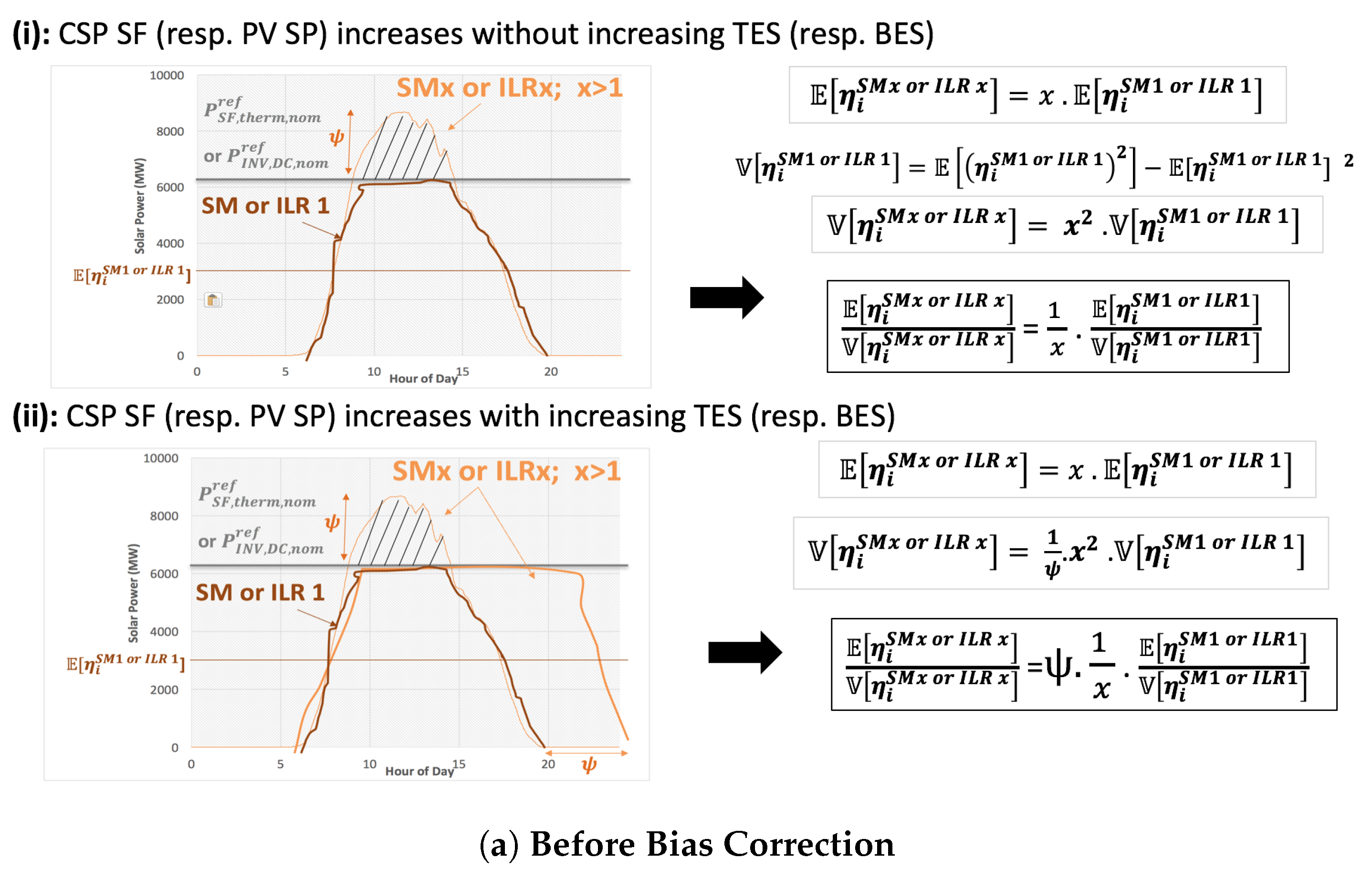
Since solar power connected to the electricity network is often contracted under a power purchase agreement, which is paid by the kilowatt hour generated, more hours of operation equals more money to amortize capital costs faster, so developers want to maximize the hours of operation each year. In order to increase the operating hours of both solar technologies, one may increase both TES (resp., BES) capacity and CSP solar field—SF—(resp., PV solar panels—SP) compared to fixed electricity-generating turbine (resp., inverter) capacity, as measured by the Solar Multiple—SM—(Inverter Loading Ratio—ILR) [48]. Therefore, not only the relative variance is reduced, but the mean of the CF is increased as well, even without storage, because the system in this case rarely produces at nominal capacity; this allows to reach a more efficient operation of the electrical generation, which reduces the operation and maintenance costs [13,49]. In addition, the adoption of TES (resp., BES) in CSP (resp., PV) plants will generally lead to increased capital costs because of the investment in storage systems, but also the cost of the additional CSP SF (resp., PV SP) that are required to produce electricity also in times when the sun does not shine. However, the greater electricity generation will generally result in a lower electricity generation cost (LCOE) [48,49,50]. Overall, the trade-off between the incremental costs of the increased storage systems size and of the additional CSP SF (resp., PV SP) must be balanced against the decrease in the variability and the revenues that will accrue from the ability to dispatch power generation at times of high demand and high electricity prices.

A key question moving forward is how to compare interaction between PV-BES and CSP-TES in a particular prospective power generation mix based on renewable energies (REs). While both technologies collect solar radiation and produce electricity, they do so through different mean production, costs and variability [51], which creates challenges for direct comparison.

Recently, the cost and storage effect that solar technologies PV and CSP with their associated storage (BES and TES) have on an energy mix have been addressed in literature. Bogdanov et al. (2015) [52] analyze the role of these technologies towards 100% RE mix. Feldman et al. (2016) [48] use a range of cost projections to compare the competitivity of PV-BES and CSP-TES through 2030. Chattopadhyay et al. (2018) [53] built a capacity planning model to evaluate the impact of the addition of PV-BES without or with spinning reserve capability on the integration of CSP-TES. Lovegrove et al. (2018) [54] examine different dispatchable generation technology combinations with regard to their development status, performance characteristics, storage capability and costs. Kumar et al. (2019) [55] present a comparative economic analysis of supplying solar PV-BES and CSP-TES power to a particular load in India. Zurita et al. (2019) [56] evaluate different dispatching strategies of a hybrid CSP-PV-TES-BES in Chile considering different seasons and locations. Papadopoulou et al. (2020) [57] assess the techno-economic performance of combination of these technologies with offshore wind with storage. Overall, these publications [48,52,53,54,55,56,57] tend to analyze the competitiveness of PV-BES with CSP-TES over a range of storage requirements and under several projected cost declines for PV, batteries and CSP, focusing only on generation costs. However, the inherent differences between these technologies cannot be examined using a single metric as both provide different grid services and different economic values. For instance, depending on the amount of storage associated, a PV-BES system may provide additional services [53,58,59] such as responding very quickly to changing system needs compared to CSP-TES which requires time to start up and ramp [48]. Alternatively, CSP-TES may allow a greater capture of solar energy, reducing the curtailment in very high solar penetration scenarios [60]. In addition, the value of dispatchable solar energy operating during peak hours—when the fuel cost of conventional generators is high—is much more important than that of solar base load plants operating only during low-load periods.

Thus, while these analyses evaluate only cost per unit of generation, additional studies focus also on the variability by considering the incremental avoided capacity and fuel costs associated with the addition of PV-BES and CSP-TES. For instance, Narimani et al. (2017) [61] compare this operational value in the Australian electricity market. Existing research tends to compare the capacity credit (i.e., the actual fraction of the generators capacity that could reliably be used to replace conventional capacity during peak hours, which is typically measured as percentage of nameplate capacity), or the effective load-carrying capacity of a plant (i.e., the capacity credit multiplied by the nameplate capacity) between PV and CSP-TES or conventional gas generators [21,62] and PV-BES [22]. Similar contributions have been made to compare the net cost or the benefits–costs ratio [22] (resp., benefits/costs) [63] determined by subtracting (resp., dividing) the annualized capital and fixed operation and maintenance costs of a generator from the system cost savings.

However, an analysis of the conditions under which each technology outperforms its counterpart within an optimization framework under different scenarios of penetrations and storage configurations considering both the cost and the storage impact on the mean penetration, variance and covariance between different renewable technologies and climate regions remains not explored. Particularly, the utilization of CSP and PV with storage is widely suggested within the Moroccan strategy that aims to deploy 20% of its electrical capacity from solar energy by 2030 [64]. However, the share between PV and CSP and the amount of storage associated is still to be found. Currently, the actual storage configuration and performance of these systems for dispatchable energy are in the early stages of being defined. In fact, renewable expansion in Morocco, with high solar resource [64], is primarily perceived in terms of opportunities, such as contribution to RE targets, reduction of carbon emissions, reducing energy dependence [64], while the issues related to cost and storage associated with solar technologies in the mix receive significantly less attention.

Choosing the technologies on the basis of cost alone (i.e., cost minimization problem) or characterizing the variability of imbalances alone (i.e., reducing the balancing needs) can be misleading [65]. These objectives are likely to be conflicting with each other. As such, an energy system based on solar technologies (PV, CSP) without and with their associated storage (BES, TES) needs a multi-objectives optimization problem that considers the whole range of feasible solutions by determining trade-offs between mean production, cost and variability. Such a trade-off can be satisfied by the “Pareto Optimal Front” of the bi-objective mean-variance optimization problem [66] used in this study. We take the existing power generation portfolio as a starting point for the analysis of possible system transformation trajectories with solar and wind energies. Our objective is to maximize the RE production at a given cost and to lower the mismatch between the demand and the RE production (i.e., the variance-based adequacy risk for the electrical grid). Increasing the mean RE penetration towards 100% tends to reduce system costs and greenhouse gas emissions by decreasing the total conventional production.

This study is a follow-up work to a previous study carried out by Bouramdane et al. (2020) [51] exploring the response of the Moroccan mix to the integration of CSP/CSP-TES with different storage capabilities with wind and PV without storage and examining the role of thermal storage and diversification in reducing the variability. In this study, the optimization problem is not only sensitive to the change of the variance associated with the change of the CSP SM and to the different rental costs of wind, PV and CSP, but also to (i) the variance associated with the change of the PV ILR and to (ii) the different rental cost of PV and CSP storage configurations. As in this previous study, we optimize the electricity mix using a recommissioning approach in which the total cost of a mix is constrained to be lower than that of the current (2018) Moroccan mix with the following analysis. We try to see what role the addition of battery to PV can play in reducing the variability and whether or not it becomes part of the mix examining its integration with CSP/CSP-TES and wind across a set of penetrations regimes and under the recent (2013) cost data. Concerning the competitiveness between PV-BES and CSP-TES, this study does not aim to identify the best technology or analyze the sensitivity of the mix to cost uncertainty, but rather to investigate the circumstances under which PV-BES could have an advantage against comparable technologies (i.e., CSP-TES) along with a range of other points of comparison in terms of rental cost and variability (i.e., load bands reduction such as the average capacity credit). Therefore, this study attempts to answer two further questions to the ones answered in [51]:

• Does the cost and storage capability of CSP-TES and PV-BES that increase with the SM and ILR introduce a significant change in the scenario mixes?
• What are the benefits of CSP combined with TES to PV deployed with BES in terms of adequacy risk (i.e., variance-based risk and load-bands-reduction diagnostics)?

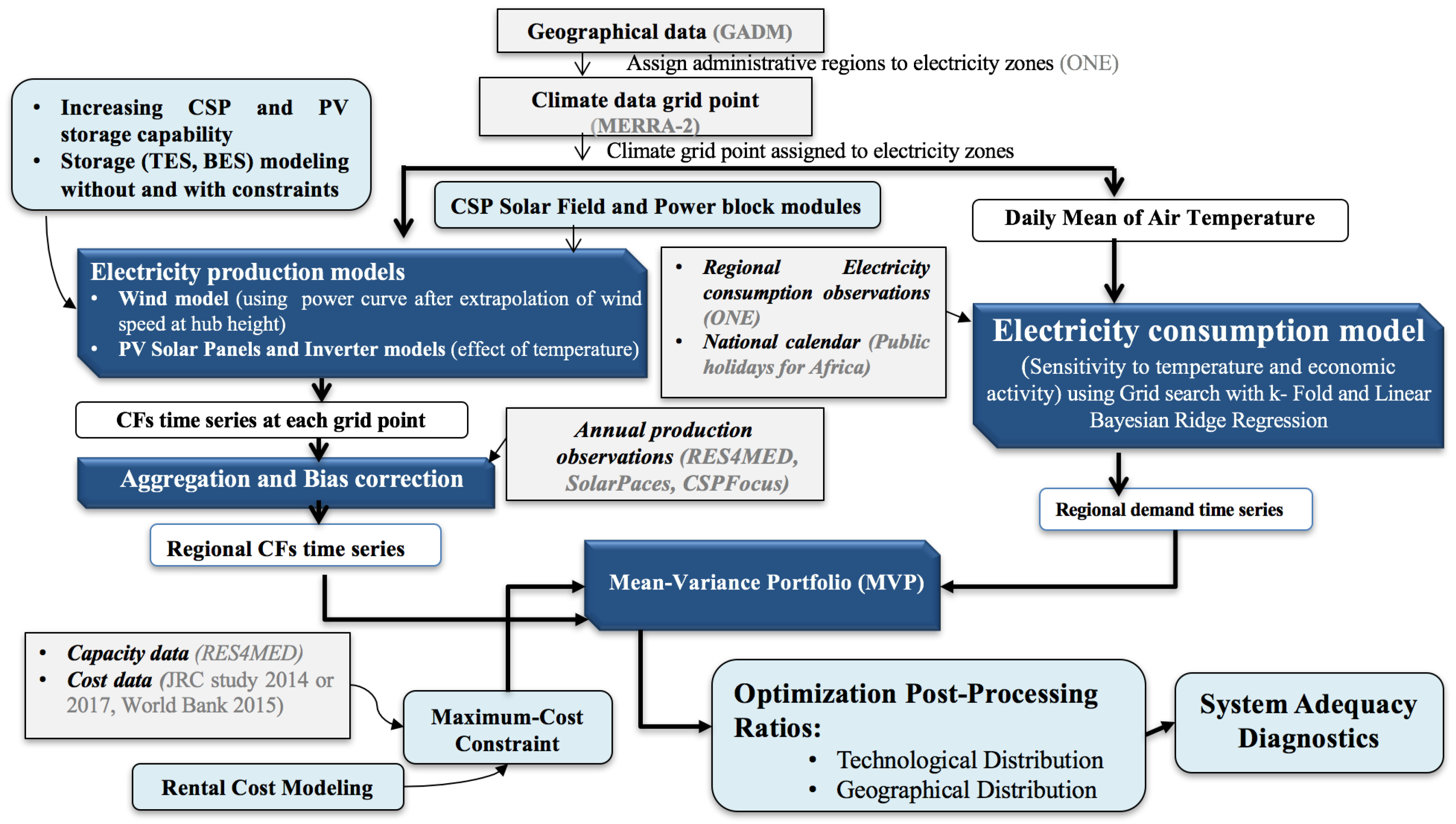
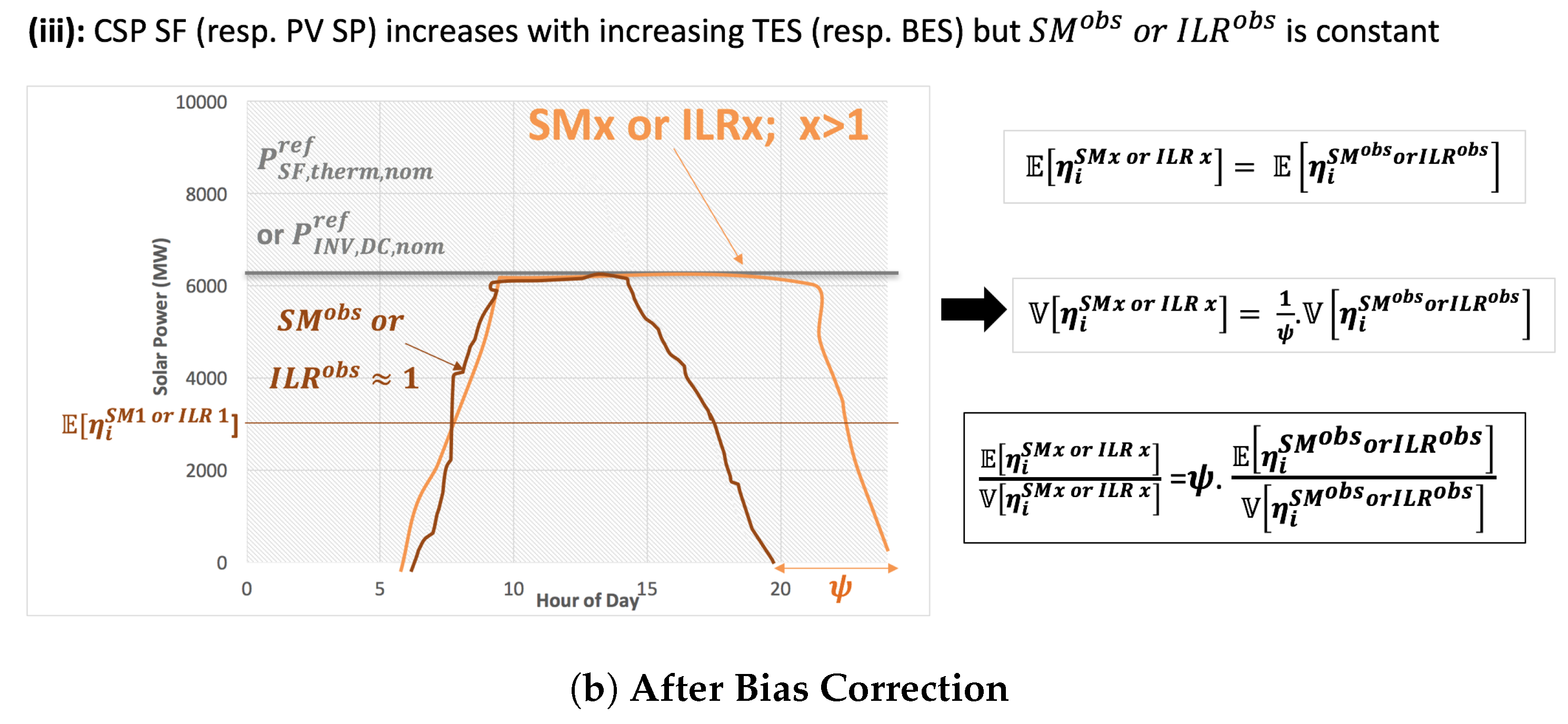
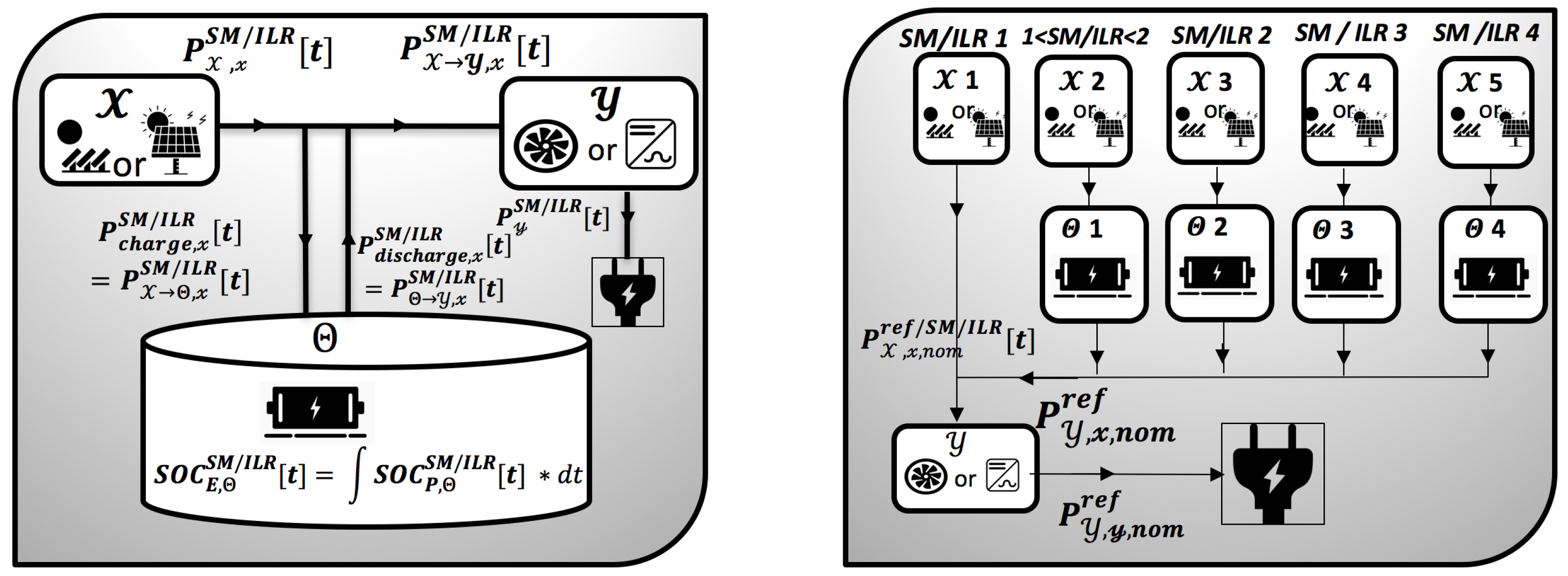
In order to find answers to the questions stated above, we use the E4CLIM model [51,67] that allows, using climate data provided by MERRA-2 reanalysis for the four Moroccan electrical zones for the year 2018, to simulate hourly wind, PV with BES, CSP without and with TES, and demand curves adjusted to observations. We address different combinations of variably sizable PV and CSP with wind. We choose similar sizing to make the technologies as comparable as possible. We develop a method of rental cost modeling in which the cost related to energy and power capacity of both storage technologies is considered, keeping the cost of CSP SF (resp., PV SP) constant to remain coherent with the fact that the mean solar CFs of different storage sizes are roughly equal due to bias correction. Therefore, an increase in the CSP SM (resp., PV ILR) gives an increase in the storage capacity and the maximum power of charging/discharging which increase the rental cost. So far, most studies are based on an uniform distribution of RE capacities. In our study, the distribution of the RE capacities is optimized technologically or geographically, or both, in order to evaluate the impact of diversification in reducing the standard deviation of the RE production.

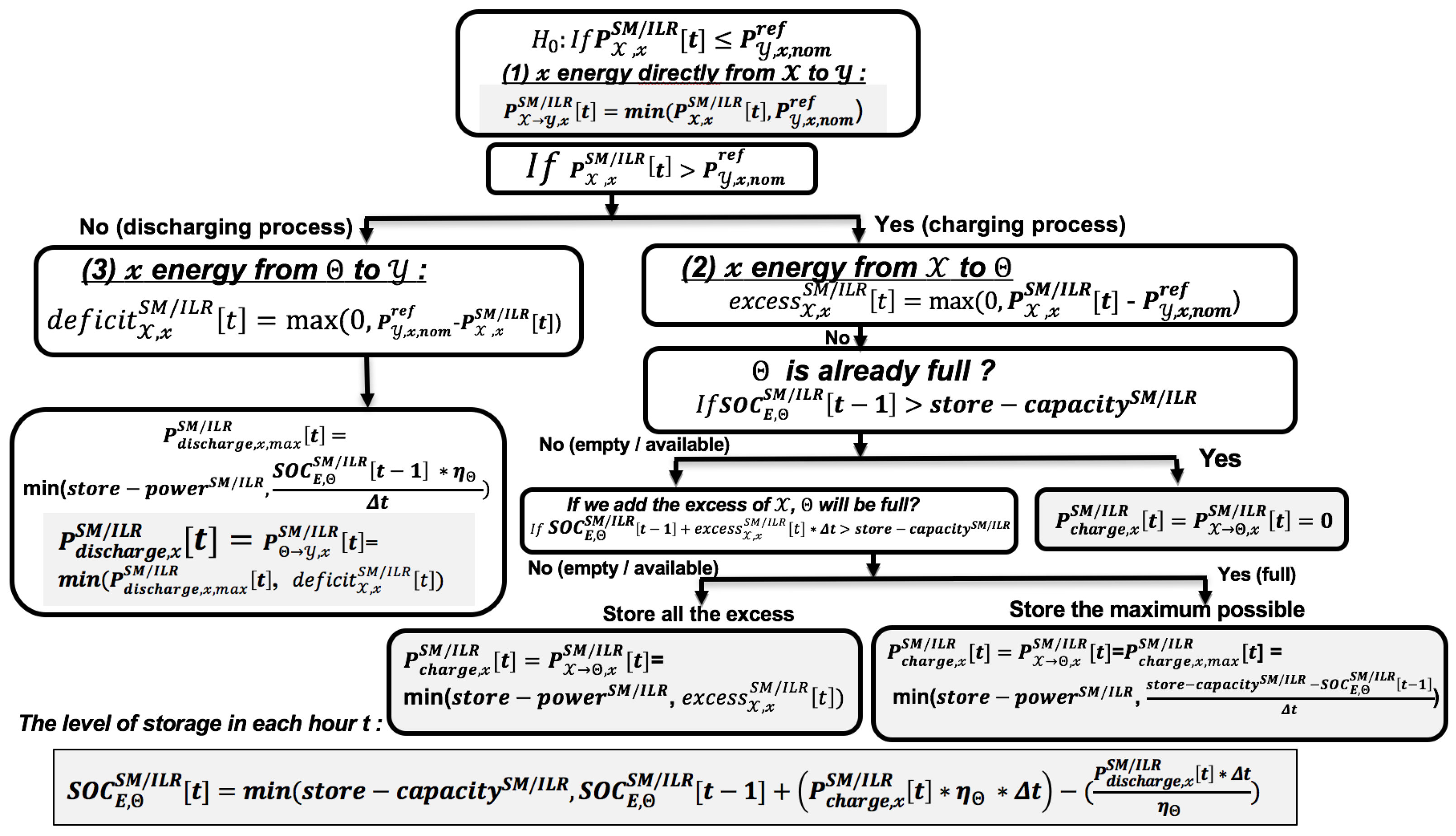
After this introduction, the remainder of this paper is organized as follows. The methodology section (Section 2) comprises different sub-sections. Section 2.1 gives an overview of our objectives and the available optimization strategies in the E4CLIM model. The remaining sub-sections present the stages of our research contribution to E4CLIM (Section 2.2), including the theoretical framework of the storage model (Section 2.3) and the cost model (Section 2.5) implemented as a special case for this study. We also present the optimization inputs (Section 2.4) and the renewable combinations considered in this study (Section 2.6). Section 3 presents the resulting optimal scenario mixes by analyzing the impact of thermal and battery storage on the technological and geographical distribution of RE capacities (Section 3.1), the impact of diversification (Section 3.2) and the role of CSP-TES compared to PV-BES in reducing the adequacy risk (Section 3.1). Section 4 summarizes the methodology adapted and the results gained for all scenarios. Points of discussion regarding the scenarios of solar integration in Morocco will be further considered before concluding the limitations of the current study and the expected future work.

2. Methodology

In this section, we give a brief description of the mean-variance optimization framework, as an alternative to the more traditional least-cost approach or minimum balancing needs approach, before describing the methodology adapted in the storage and rental cost models.

The flow chart given in Figure 1 summarizes the components of E4CLIM (dark blue), including the modules added (light blue) and the data sources (gray) to illustrate briefly the general framework of this study.

2.1. Objective Functions and Optimization Strategies in E4CLIM Model

The bi-objective optimization problem aims at maximizing the mean penetration (1) and minimizing the aggregate RE supply risk squared ${\sigma }_{\mathrm{global}\left|\mathrm{technology}\right|\mathrm{strategy}}^2$ of the mix; using three versions of the variance: global variance (2) of energy generation ${\eta }_k\left(t\right)·{\omega }_{\mathit{k}}$ considering covariances between time-dependent predicted CFs, ${\eta }_k\left(t\right)$—normalized by the total predicted demand ${\sum }_i{D}_i\left(t\right)$—for a pair $k=(i,j)$ of different production technologies j in different zones i; technology strategy (3) where only covariances between technologies of the same zone are considered; and base strategy (4) where all covariances are set to zero. Comparing mixes from these strategies allows us to assess the benefits from technological and geographical diversification. For instance, having non-zero installed capacities, ${\omega }_{\mathit{k}}$, in two negatively correlated region–technology pairs produces lower risk than in cases in which they are positively correlated or even uncorrelated (right side of Equation (2)).

$$\mu \left(\mathbf{w}\right):=\mathbb{E}\left[\sum _k{\omega }_{\mathit{k}}\frac{{\eta }_k\left(t\right)}{{\sum }_i{D}_i\left(t\right)}\right]=\sum _k{\omega }_{\mathit{k}}\mathbb{E}\left[\frac{{\eta }_k\left(t\right)}{{\sum }_i{D}_i\left(t\right)}\right].$$

(1)

$${\sigma }_{\mathrm{global}}^2\left(\mathbf{w}\right):=\mathbb{V}\left[\sum _k{\omega }_{\mathit{k}}\frac{{\eta }_k\left(t\right)}{{\sum }_i{D}_i\left(t\right)}\right]:=\sum _k{\omega }_{\mathit{k}}^2\mathbb{V}\left[\frac{{\eta }_k\left(t\right)}{{\sum }_i{D}_i\left(t\right)}\right]+\sum _{k\ne l}{\omega }_{\mathit{k}}{\omega }_{\mathit{l}}\mathrm{Cov}\left[\frac{{\eta }_{\mathit{k}}}{{\sum }_i{D}_i},\frac{{\eta }_{\mathit{l}}}{{\sum }_i{D}_i}\right].$$

(2)

$$\begin{array}{cc}\hfill {\sigma }_{\mathrm{technology}}^2\left(\mathbf{w}\right)& :=\sum _i\mathbb{V}\left[\sum _j{w}_k\frac{{\eta }_k\left(t\right)}{{\sum }_i{D}_i\left(t\right)}\right]\hfill \end{array}$$

(3)

$$\begin{array}{cc}\hfill {\sigma }_{\mathrm{base}}^2\left(\mathbf{w}\right)& :=\sum _{\mathbf{k}}\mathbb{V}\left[w_{\mathbf{k}}\frac{{\eta }_{\mathbf{k}}\left(t\right)}{{\sum }_i{D}_i\left(t\right)}\right]\hfill \end{array}$$

(4)

$\mathbb{E}$, $\mathbb{V}$ and $Cov$ represent respectively the mathematical expectation, variance and covariance operators over time; and ∑ is the sum over the index in subscript.

For each strategy, an optimal mix is obtained by minimizing the variance for a given desired mean penetration or vice versa ([67], Appendix B). Therefore, the mean-variance approach does not provide a single optimal mix but several optimal choices, referred to as the optimal frontier curve ($\mu$(ŵ), $\sigma$(ŵ)) visualized in the mean-standard deviation graph, where ŵ denotes the vector with components giving the optimal installed capacities, ${\omega }_{\mathit{k}}$, for a zone–technology pair k. This allows for more space to arbiter between different mixes with a large share of renewable energies and mixes requiring less flexibility.

This mean-variance bi-objective problem is implemented in the E4CLIM model that allows to compute wind, solar PV production, energy demand adjusted to observations by using geographical data for specific area and climate data, and to optimize the renewable electricity mix; taking into account the time–space variability of both the generation and the demand [67].

2.2. Model Set-Up and Additional Modules to E4CLIM Model

2.2.1. Domain and Calibration

We adapt the E4CLIM model to Morocco and its four electrical zones i={NORTH, CENTER, EAST, SOUTH} for the year 2018 by calibrating it with Morocco’s data. The geographical, climate, demand and CFs data are described in ([51], Section 2.6).

The accuracy of the mean-variance analysis (Section 2.1) depends on the inputs of this optimization problem, namely, the vector of mean solar and wind capacity factors (CFs) and demand time series entering the definition of the mean penetration (1) and of the variance (2). To correct bias that stems from climate simulations, real hourly renewable (RE) production time series per zone and technology are required. These data are difficult to acquire at regional level and in appropriate intervals in Morocco, since the deployment of RE capacity is relatively recent in Morocco (it started in 2009 but not until 2016 for solar CSP) [68]. The RE production and capacity data used in this study were provided by recent literature research on a yearly basis. However, while knowing a single averaged value over the region is useful, this may not be sufficient to correct low-frequency climate variability of electricity production. On the other hand, from a climate perspective, the analyses of long-term climate data can have a substantial impact on the design of electricity mixes [69]. Accordingly, we estimate the CFs and demand over the whole period (1981–present day) available from the MERRA-2 reanalysis climate data [70]. Since the inter-annual variability of the mean CFs and mean demand (inputs of the optimization) from 1981 to 2019 were found to be weak (not shown here) and since the length of the regional observed demand time series is limited to one year (2018) on an hourly basis and only means of observed CFs over the same year are available, we consider that the climate over the period 1981–2019 is represented by the year 2018 to correct bias in the production models and fit the demand model. Running the MERRA-2 climate reanalysis on only one year can be very misleading. The simulations are independent of the chronicles of past years. The shorter the time horizon, the larger variation the is in the average, because there is an averaging effect when considering a large time horizon. Due to lack of high-quality data, our analyses are carried out over one year spanning the period from January 2018 to December 2018 to improve the bias in the variance of the CFs since our objective is to analyse the sensitivity of the mix to storage and cost associated with solar technologies and not to find the long-term planning for system capacity (i.e., how much capacity is needed in order to meet greater demand).

2.2.2. CSP-TES and PV-BES Simulation Modules

To study the response of the optimal mix to the integration of CSP without/with storage and to the addition of storage to PV, we develop solar modules to E4CLIM to simulate the thermal (resp., Direct Current, DC) energy provided by either the CSP solar field (resp., PV solar panel) or the thermal (resp., battery) storage system and the electricity produced by the CSP power block (resp., PV inverter). See ([51], Section 2.3) for CSP and Appendix A for PV.

In our study, parabolic trough (PT) was selected because it represents today’s most widespread CSP technology [49], in particular in Morocco [71,72,73], with continuous north–south tracking as it is relevant orientation for locations with a high summer peak and with relatively large seasonal irradiation variance [74,75,76] (i.e., Morocco, see Section 3.1.4).

For PV, a multi-crystalline technology is used due to its large market share [77]. Unlike CSP, the PV surface is not tracked-horizontal, it is fixed-tilted up toward the South horizon by an angle equal to the local latitude. This orientation is often selected since it averages the noontime irradiation peaks over the year [75,78] to maximize the annual energy produced, particularly in Morocco [79].

Due to weather and clouds, we rarely obtain the nominal conditions ratings from a solar CSP (resp., PV) plant. Therefore, an appropriate storage strategy is needed. A very common storage strategy is to save energy stored for a time when the electricity prices and demand are high to achieve maximum revenues and only the remaining energy that the storage cannot admit goes to the turbine (resp., inverter) (e.g., for CSP [80,81]). However, this operation strategy needs the ability to react very quickly to price fluctuations and only operate during peak load hours, so that a low capacity factor (CF) is achieved. However, to maximize the RE penetration (1), one has to maximize the power output throughout the day and night (if possible). Unlike CSP-TES, there have been no large-scale deployments of PV with BES systems designed to provide dispatchable energy. Therefore, the concepts and nomenclature of solar-plus-storage plant configurations are better established for CSP-TES than for PV-BES. For the sake of simplicity, we illustrate in Section 2.3.1 the general approach used to increase the full-load operating hours of CSP and PV by referring to related equivalent terms. In addition, Section 2.3.2 presents the storage model implemented to the thermal and battery storage combined with CSP and PV, where for each storage configuration, we follow the nominal thermal (resp., DC) capacity in order to maximize the CSP (resp., PV) CFs.

We assume that, apart from onshore wind, solar PV and CSP, both without or with storage, no other renewable (RE) technology takes part of the electricity generation; and the difference between the demand and the RE production is taken into account in the mean (1) and risk (2) of the mean variance, used as proxies for the system adequacy services needed from the conventional plants or other flexibility options (imports, demand-response mechanisms, etc.) Thus $j=\{PV,Wind,CSP\}$, and $j\prime =\{BES,TES\}$. The multi-index is thus either $k=(i,j)$ if no storage or $k=(i,j,j^{\prime })$ if storage is integrated.

2.2.3. Cost Modules

To take into account the differences in rental cost between PV, wind, CSP technologies, we use the maximum-cost constraint (5) added to the optimization problem in addition to the constraint preventing RE capacities to be negative ${\omega }_k\ge 0\forall k$. Thus, we allow the model to recommission PV, wind and CSP capacities at a cost limited by the total cost of capacities ${\omega }_{\mathit{k}}^{obs}$ for all k (5) installed in Morocco in 2018 corresponding to the most widely deployed system in Morocco (PV-Wind-CSP-TES combination with 5.5 h of TES):

$$\sum _{\mathit{k}}{\omega }_{\mathit{k}}{c}_{\mathit{k}}\le C_{\mathrm{tot}}^{obs}$$

(5)

The quantity $c_{\mathit{k}}$ is the rental cost which corresponds to the total discounted costs of installing and operating given system over its lifetime, in €/MW/yr [82].

After bias correction, we found that the means of solar CFs for different storage sizes have similar values (Section 2.4) because all the operational CSP (resp., PV) plants have similar CSP SF (resp., PV SP) size (as defined by CSP Solar Multiple—SM—or PV Inverter Loading Ratio—ILR) even though they have different storage durations (Appendix C.2). Therefore, in our previous study [51], the rental cost of CSP is also kept the same for different SMs and we proposed a definition of rental cost, $c_{\mathit{k}}$, that implicitly accounts for the TES cost (6) considering the rental cost of the whole CSP-TES plant—corresponding to the Andasol plant with 6–8 h of storage on average, for which cost data are available. In this case, the TES constraints are ignored in the storage model and only operational CSP plants with 7 h of TES are selected to correct bias in the mean CSP CFs and to compute the maximum-cost constraint (5). The cost data in this case come from the scenario-based cost trajectories to 2050 [83] of the European Commission Joint Research Center (JRC) for the year 2015.

$$\begin{array}{c}\hfill c_k:=c_{j,j_{6-8h}^{\prime }}={\sum }_{t=1}^{Lifetim{e}_{j,j_{6-8h}^{\prime }}}\frac{CAPE{X}_{j,j_{6-8h}^{\prime }}+OPE{X}_{j,j_{6-8h}^{\prime }}}{{(1+D{R}_j)}^t}.\end{array}$$

(6)

The terms CAPEX and OPEX are, respectively, the capital and operational expenditures over the lifetime of the plant; DR is the discount rate.

Doing so, the optimization problem is only sensitive to the change of the variance associated with the change of the SM and to the different rental costs of wind, PV and CSP. However, the costs per installed capacity of CSP and PV plants utilizing storage with several hours will be much higher than those of plants without storage or with smaller amounts of storage. Therefore, evaluating a specific technology j or $j,j^{\prime }$ in the mix requires calculating the technology rental cost $c_j$ but also the storage rental cost $c_{j^{\prime }}$. For this reason, a different rental cost formulation is implemented in this study (Section 2.5). Therefore, to take into account the increased cost related to increased storage size, we have to apply constraints on the storage capacity and the maximum power of charging/discharging in the storage model (Section 2.3.2).

2.3. Storage Modeling

The left panel of Figure 2 represents a block diagram of a CSP-TES (resp., PV-BES) plant components. The left-corner block is the CSP Solar Field—SF— (resp., PV Solar Panel—SP) providing thermal (resp., Direct Current—DC) output; the corner block on the right is the CSP Power Block–PB—(resp., PV Inverter—INV) providing the electrical output. To the bottom is the Thermal (resp., Battery) Energy Storage system (i.e., TES and BES). The black arrows represent thermal/electrical flows to illustrate the meaning of each parameter calculated. To simplify, let us consider $\mathit{X}=\{SF,SP\}$; $\mathit{Y}=\{PB,INV\}$; $\Theta =\{TES,BES\}$; $\mathit{x}=\{therm,DC\}$; and $\mathit{y}=\left\{elec\right\}$.

2.3.1. CSP Solar Multiple and PV Inverter Loading Ratio

Several sizing approaches exist depending on the desired type of plant (i.e., base, peak or intermediate plant, etc.) [78,84]. In our study, we hold the CSP PB (resp., PV INV) fixed and size the CSP SF (resp., PV SP) and Thermal (resp., Battery) storage system in relation to the PB (resp., INV). In other words, we install more thermal (resp., DC) power capacity on a PB (resp., INV) system than their power rating (right panel of Figure 2). The ratio between the thermal (resp., DC) power produced by the CSP SF (resp., PV SP) and the thermal (resp., DC) power required by the PB (resp., INV) at nominal conditions is called the Solar Multiple—SM (resp., Inverter Loading Ratio—ILR) [48,84].

These parameters are proportional to the number of hours of production from the thermal (resp., DC) energy stored. There is, however, an indirect relationship between the SM (resp., ILR) and the storage size: The higher the SM (resp., ILR), the higher is the aperture area of collectors in the SF (resp., SP) (7) which require larger storage capacity:

$$A_{\mathit{X}}^{SM/ILR}:=\frac{SM/ILR\ast P_{\mathit{X},\mathit{x},\mathit{nom}}^{ref}}{{\eta }_{\mathit{X},\mathit{nom}}^{ref}\ast S}=A_{\mathit{X}}^{ref}\ast \frac{SM/ILR}{S{M}^{ref}/IL{R}^{ref}}$$

(7)

where $S=\{DirN{I}_{DP},GT{I}_{STC}\}$ is the direct normal irradiation at the design point; and the global tilted irradiation at standard test conditions which are needed, respectively, by CSP and PV. The term, $P_{\mathit{X},\mathit{x},\mathit{nom}}^{ref}$, is the thermal (resp., DC) nominal capacity. The quantities $A_{\mathit{X}}^{ref}$, ${\eta }_{\mathit{X},\mathit{nom}}^{ref}$ and $S{M}^{ref}/IL{R}^{ref}$ are, respectively, the reference CSP SF (resp., PV SP) area, efficiency and CSP SM (resp., PV ILR) [85].

Unlike PV, almost all CSP plants being developed in Morocco are with storage ([51], Table A4). In our study, the reference configuration of TES is that of the 50 MW plant Andasol 1 ([51], Table A1) with $S{M}^{ref}$ that we found equal to 1.87, meaning that the SF delivers 87% more thermal energy than is required to generate the nominal power. The 87% excess energy can be delivered to TES. We also consider SMs of 2, 3 and 4 by increasing $A_{\mathrm{SF}}^{SM}$ proportionally from its reference value using Equation (7). A case without storage is also considered, in which the area, $A_{\mathrm{SF}}^{SM}$, is set for SM equal to 1.

For PV, the case without storage, $IL{R}^{ref}=1$, has been chosen as reference configuration. For the sake of comparison between PV-BES and CSP-TES, ILR of 2, 3, 4 are considered. With CSP SM4 (resp., PV ILR4), the plants are able to run at nearly constant output (Section 3.1.4). Therefore, further increasing CSP SM (resp., PV ILR) does not make sense, as during high irradiation periods they would lead to increasingly unused surplus energy.

2.3.2. Storage Model Approach

In our study, the storage model is based on a set of dispatch conditions (Figure 3) that takes into account the frequency of charging and discharging instead of relying on heuristics or optimization problems [86], or applying a moving average filter [87] often used to smooth the hourly daily fluctuations.

CSP production tends to produce more in grid cell with the most favourable solar resource conditions, and often a minor portion of a grid points with high irradiation may host enough installed capacity. Considering this, a higher percentile instead of the average could better illustrate the storage capacity, $store-capacit{y}^{SM/ILR}$, and the maximum power of storage, $store-powe{r}^{SM/ILR}$. These parameters are respectively calculated as the 95th percentile for the state of charge, $SO{C}_{E,\Theta }^{SM/ILR}$, and the energy charged, $P_{\mathit{X}\to \Theta ,x}^{SM/ILR}$, for all climate grid points over 1 year (2018) by running the storage model without constraints.

In fact, the storage model without constraints compared to the one with constraints (Figure 3) assumes that the storage system is never full, even after putting the CSP SF (resp., PV SP) excess, and is thus always available (i.e., empty or half-empty storage). That is to say, that the storage system is always over-dimensioned to explore the solar resource and maintain full output (Appendix B). The model with constraints assumes that the storage system can be already full if the state of charge, $SO{C}_{E,\Theta }^{SM/ILR}$, exceeds the storage capacity at some time spell $t-1$, so that $P_{\mathit{X}\to \Theta ,x}^{SM/ILR}=0$. Thus, the storage system is no longer always available. In case the storage system is full after adding the excess of SF (resp., SP), we store the maximum possible; otherwise, we store all the excess while satisfying the storage constraints. The state of charge, $SO{C}_{E,\Theta }^{SM/ILR}$, is thus now limited by the storage capacity and the maximum power of charging or discharging that depends on the surface of the SF (resp., SP) $A_{\mathit{X}}^{SM/ILR}$ (7) and thus on the SM (resp., ILR). An overview of the charging and discharging daily operation of the CSP-TES configuration with $S{M}^{ref}$ (5.5 h of storage) can be found in ([51], Figure 1 in Section 2.3.3).

The storage duration per day on average (8) is calculated by subtracting the mean CF of the plant with storage from the one without storage. The resulting TES and BES parameters are given in

Table 1. Storage parameters: Storage capacity (MWh) (first column), Maximum power of charging/discharging (MW) (second column), Total energy discharged (TWh) (third column) and Storage duration (h/day) (fourth column) obtained for TES and BES model without constraints (Appendix B).

SM/ILR	TES/BES Parameters
	$\mathit{store}-{\mathit{capacity}}^{\mathit{SM}/\mathit{ILR}}$	$\mathit{store}-{\mathit{power}}^{\mathit{SM}/\mathit{ILR}}$	$\sum {\mathit{E}}_{\mathit{discharged}}^{\mathit{SM}/\mathit{ILR}}$	${\mathit{h}}^{\mathit{SM}/\mathit{ILR}}$
$S{M}^{ref}$	649	149	36.5	5.48
SM2	754	169	42.7	6.13
SM3	1648	325	94.2	11.2
SM4	52,793	480	148.3	17.2
ILR2	794 × 10${}^{-6}$	183 × 10${}^{-6}$	47.4 × 10${}^{-3}$	4.73
ILR3	2038 × 10${}^{-6}$	399 × 10${}^{-6}$	122.7 × 10${}^{-3}$	9.13
ILR4	4909 × 10${}^{-6}$	616 × 10${}^{-6}$	201.8 × 10${}^{-3}$	13.4

.

$$h^{SM/ILR}=\frac{(\overline{{\eta }_{i,j,j^{\prime }}}-\overline{{\eta }_{i,j}})\ast 8760}{365}$$

(8)

2.4. Predicted Demand and Bias-Corrected Capacity Factors

The hourly wind, PV-BES and CSP/CSP-TES capacity factors (CFs) are obtained by dividing the computed production by its nominal value at each climate grid point. These time series are then aggregated at regional level and statistically adjusted to observations ([51], Section 2.6.4).

In this study, all operational CSP and PV plants are considered for bias correction and to compute the maximum-cost constraint (5) (Appendix C.1), although PV and CSP technologies, tracking options and storage configurations are different from the ones considered in this study which prevents validating CFs estimates against observations. Due to the lack of better-quality data, these annual production data are, at the moment, the best source of information.

The yearly means of the predicted regional demand and bias-corrected CFs are reported in

Table 2. Regional predicted yearly demand (MWh/yr) and bias-corrected solar and wind CFs (%) averaged over the year 2018 per zone and technology. SM1: CSP without storage; ILR > 1 or SM > 1: with increasing levels of storage.

Zones	Demand	Wind	PV			CSP
			ILR2	ILR3	ILR4	SM1	SM2	SM3	SM4
NORTH	450.55	37.8	19.5	19.5	19.3	30.4	31.0	31.0	30.8
CENTER	3726.52	40.0	19.5	19.5	19.5	38.8	38.8	38.8	39.0
EAST	224.28	47.3	21.0	21.0	21.0	31.4	31.4	31.4	31.4
SOUTH	90.0	46.0	21.6	21.6	21.7	37.0	37.0	37.0	37.0

. From this table, we can see that the mean CFs are larger for wind than for CSP/CSP-TES, and larger for CSP whatever the SM than for PV/PV-BES whatever the ILR because observed solar PV-BES and CSP/CSP-TES have the same ILR and SM (Appendix C.2).

2.5. Rental Cost Modeling and Data

In this study, we propose a method, based on the Net Present Value method [82] (instead of the annuity factor method [85]) to calculate the rental cost of the generation and storage technologies based on the available cost parameters. An essential point on which we build is that the rental cost of CSP-TES (resp., PV-BES) has to be defined relative to the SM (resp., ILR) to take into account the cost of the additional CSP Solar Field—SF (resp., PV Solar Panel—SP) and the amount of storage associated.

In fact, it is commonly known that an increase in the Solar Multiple—SM (resp., Inverter Loading Ratio—ILR) does not give a proportionate increase in the hours of storage. For instance, the CSP SF (resp., PV SP) can be oversized without investing in the TES (resp., BES) and vice versa, which does not give a proportionate increase in the CFs and thus a proportionate reduction in generation costs [48,49,50].

In this study, the amount of storage and CSP SM (resp., PV ILR) are matched with one another, i.e., an increase in the CSP SM (resp., PV ILR) results in an increase in the CSP SF (resp., PV SF) which increase the storage capacity (Section 2.3.1, Table 1). Moreover, the CFs are kept constant for all SMs (resp., ILRs) due to the bias correction (Section 2.4). In fact, having mean CFs that change very little with increasing SM (resp., ILR) avoid to increase the variance—associated with the increase of the CF means (quadratic term against linear term)—due to the increase of the surplus of energy available for storage with the increase of CSP SF (resp., PV SP) size (Figure A2a(i)), and this despite the reduction in the variability associated with storage (Figure A2a(ii)). With fixed mean CFs, the mean of the CF time series of CSP SM2, for instance, will be similar to CSP SM1 but the difference in the amplitude is taken in the penetration (1) and they will be penalized differently. Thus, the model would not penalize CSP SM2 against CSP SM1 just for having larger average CF. In this case, the model is only sensitive to the reduction in the variance associated with storage (Figure A2b(iii)) and to the cost associated with the change of SM and ILR.

Fixed-mean CF implies keeping the rental cost $c_j$ of CSP (SF + PB) or PV (SP + INV) constant for all SMs and ILRs. However, as a matter of fact, ignoring the differential effect that the storage (TES or BES) cost of each solar technology undermines the identification of truly optimal technology to install for each penetration level. Accordingly, we assume that the cost of the CSP-TES and PV-BES rise almost in proportion with the size of the plant (i.e., SM and ILR), i.e., storage parameters (Table 1), and the cost of additional CSP SF and PV SP can be scaled without incurring much additional cost (in line with [88]).

This assumption reported here appear to support the assumption that CSP or PV plants utilizing storage with several hours will be much larger, which contributes implicitly to much higher cost per installed capacity, even though the mean CFs are fixed. However, it is important to bear in mind that for CSP, the SF is by far the largest cost component of parabolic trough plants and accounts for 38.5% of the total installed costs (looking at the 50 MW PT Andasol plant with 7.5 h, taken as reference plant in our study), while TES costs land at the third place after the PB and grid connections costs (see a detailed breakdown of the investment cost [49], Table 4.2). The same goes for PV, the cost of the PV module is higher than that of the inverter [13].

The yearly rental cost, $c_k$, is thus the sum of the yearly rental cost of the production technology, $c_j$, and the yearly rental cost of the storage technology, $c_j^{\prime }$, as presented in Equation (9):

$$c_k:=c_j+c_{j^{\prime }}$$

(9)

The yearly rental cost of the generation technology, $c_j$ (10), is computed from the lifetime capital investments cost ($CAPE{X}_j$), the lifetime fixed and variable operation and maintenance cost ($FO{M}_j$ and $VO{M}_j$, respectively)–which are both annualized–, the discount rate (DR) and the lifetime ($lifetim{e}_j$).

$$c_j=\sum _{t=1}^{Lifetim{e}_j}\frac{CAPE{X}_j+[FO{M}_j+{\alpha }_{j}VO{M}_j]}{{(1+DR)}^t}$$

(10)

The yearly rental cost of the storage technology, $c_j^{\prime }$, is calculated using Equation (11). In fact, the storage system CAPEX is divided into power-related cost ($CAPE{X}_{P,j^{\prime }}$), which is the cost of power of charging/discharging, and energy-related cost ($CAPE{X}_{E,j^{\prime }}$), which is the cost of energy storage capacity or volume [89]. $FO{M}_{j^{\prime }}$ and $VO{M}_{j^{\prime }}$ are, respectively, the fixed and variable OPEX, and $lifetim{e}_{j^{\prime }}$ is the lifetime of the technology $j^{\prime }$.

$$c_{j^{\prime }}:=\sum _{t^{\prime }=1}^{Lifetim{e}_{j^{\prime }}}\frac{[{\alpha }_{j^{\prime }}CAPE{X}_{E,j^{\prime }}+{\beta }_{j^{\prime }}CAPE{X}_{P,j^{\prime }}]+\left[{\beta }_{j^{\prime }}FO{M}_{j^{\prime }}\right]}{{(1+DR)}^{t^{\prime }}}+{\gamma }_{j^{\prime }}\sum _{t^{\prime }=1}^{Lifetim{e}_{j^{\prime }}}\frac{VO{M}_{j^{\prime }}}{{(1+DR)}^{t^{\prime }}}$$

(11)

All the parameters are explained in Appendix D.

Except for the discount rate, the economic data needed to compute the yearly rental cost (9) come from the ETRI 2014—Energy Technology Reference Indicator projections for 2010–2050 [83]—of the European Commission Joint Research Center (JRC) for the year 2013. We have considered the following power production technologies j: solar thermal electricity power plants without thermal storage; commercial solar PV (more than 2MW) without tracking; and onshore wind. For storage technologies $j^{\prime }$, we have considered thermal energy storage for concentrating solar power applications and Li-ion storage battery for power grid applications.

The total cost is critically dependent upon the choice of the discount rate. Usually, low DRs are used when evaluating RE technologies [90]. A real DR of 4% in Morocco for modelling purposes seems reasonable ([90], p. 27). CSP would require a somewhat higher rate, a value of 5% [90], as also considered in [86], so a value of 4.5% is used in this study for all production and storage technologies.

This cost data are summarized in

Table 3. Capital investment, fixed and variable operation and maintenance costs, lifetime of the production technologies (Top) and storage technologies (Bottom). These data are from the ETRI 2014—Energy Technology Reference Indicator projections for 2010–2050 technical report for the year 2013 ([91], Tables 4, 7 and 10) for PV, wind and CSP; and ([91], Tables 66 and 61) for TES and Li-ion BES. The discount rate was obtained from the World Bank Report ([90], p. 27), ${\alpha }_j$ is the yearly-mean CF in (h) of the technology j (A9), and the yearly rental cost per technology, $c_j$ (€/kW/yr), is calculated using Equation (10).

Technology j	CSP		PV		Wind
$CAPE{X}_j$ (€/kW)	5600		980		1400
$FO{M}_j$ (% $CAPE{X}_j$)	4		1.7		2.7
$VO{M}_j$ (€/MWh)	8		0		–
Discount Rate $DR$ (%)	4.50		4.50		4.50
$Lifetim{e}_j$ (years)	30		25		20
${\alpha }_j\left(h\right)$	2240.91		1926.93		2147.73
Yearly Rental Cost $c_j$	3314.68		617.74		977.22
Technology j${}^{\prime }$	TES			BES
$CAPE{X}_{E,j^{\prime }}$ (€/kWh)	24			752
$CAPE{X}_{P,j^{\prime }}$ (€/kW)	1200			490
$FO{M}_{j^{\prime }}$ (%$cape{x}_{P,j^{\prime }}$)	0.2			1.4
$VO{M}_{j^{\prime }}$ (€/MWh)	–			2.6
$Lifetim{e}_{j^{\prime }}$ (years)	20			10

. The resulting yearly rental cost (9) calculated using Equations (10) and (11) are summarized in

Table 4. The yearly rental cost $c_k$ (9) (€/kW/yr) per production technology j or production technology with its storage technology $j,j^{\prime }$ calculated using Equations (10) and (11); and using storage parameters (Table 1). SM1: CSP without storage; ILR > 1 or SM > 1: with increasing levels of storage.

Techno.	Wind	PV			CSP
		ILR2	ILR3	ILR4	SM1	SM2	SM3	SM4
$c_k$	977	3380	7596.5	16,008.5	3315	6324	9165	28,399.5

. These results show that the rental cost of wind is greater than that of PV but is relatively comparable, while it is more than three times lower than that of CSP. In addition, the more the CSP SM (resp., PV ILR) increases, the more the cost of CSP (resp., PV) increases. The rental cost range of CSP-TES is by far the largest, while PV-BES presented the lowest range. For instance, for the same design (SM2 vs. ILR2 or SM4 vs. IL4), rental cost estimates for CSP-TES extend to roughly double the rental cost of PV-BES.

Injecting the cost (Table 4) and capacity data (

Table A1. Reference capacities, ${\omega }_{\mathit{k}}^{obs}$, (Left) and yearly-mean generation, $Pro{d}_{y,k}^{obs}$, (Right) per zone and technology installed in Morocco in 2018 ([51], Table A4). Zone–technology pairs for which no capacity is installed are marked by an empty set ∅.

Zone	${\mathit{\omega }}_{\mathit{k}}^{\mathit{obs}}$ (MW)			Zone	${\mathit{Prod}}_{\mathit{y},\mathit{k}}^{\mathit{obs}}$ (GWh)
	Wind	PV	CSP		Wind	PV	CSP
NORTH	396.1	∅	0	NORTH	1312	∅	∅
CENTER	60.0	70.0	510	CENTER	210	120	1734
EAST	∅	∅	20	EAST	∅	∅	55
SOUTH	759.6	100	∅	SOUTH	3056	190	∅

on the left) in (5) yields a maximum total cost, $C_{\mathrm{tot}}^{obs}$, of 3.50 G€/yr, corresponding to the PV-Wind-CSP-TES $S{M}^{ref}$ mix (with 5.5 h of TES).

2.6. Optimization Experiments

To investigate the response of the Moroccan mix to the addition of utility-scale PV combined with battery to the designed CSP with TES both with different storage capabilities—as defined by the PV ILR and CSP SM–, the optimization problem has been applied to different technological combinations (

Table 5. Optimization experiments.

Combination	Wind	CSP		PV
		TES	SM	BES	ILR
PV-ILR2-wind-CSP-SM1	Yes	No	1	Yes	2
PV-ILR3-wind-CSP-SM1	Yes	No	1	Yes	3
PV-ILR4-wind-CSP-SM1	Yes	No	1	Yes	4
PV-ILR2-wind-CSP-SM2	Yes	Yes	2	Yes	2
PV-ILR3-wind-CSP-SM2	Yes	Yes	2	Yes	3
PV-ILR4-wind-CSP-SM2	Yes	Yes	2	Yes	4
PV-ILR4-wind-CSP-SM3	Yes	Yes	3	Yes	4
PV-ILR2-wind-CSP-SM4	Yes	Yes	4	Yes	2
PV-ILR3-wind-CSP-SM4	Yes	Yes	4	Yes	3
PV-ILR4-wind-CSP-SM4	Yes	Yes	4	Yes	4

). These combinations are chosen to represent the general trend of the competitiveness of various PV and CSP storage configurations along the efficient capacity pathways.

All combinations are optimized using the same value, $C_{\mathrm{tot}}^{obs}$, i.e., 3.5 G€/yr.

3. Results

In this section, we analyze the effect that the battery added to PV has on the optimal mixes studied in ([51], Section 3) considering the differences in the variance and rental cost between not only PV, wind and CSP, but also between different SMs and ILRs.

3.1. Impact of Storage and Cost: Technological and Geographical Distribution

Approximations of the optimal fronts of the mean-variance bi-objective optimization problem are represented in the left panels of Figure 4 and Figure 5, with the standard deviation or risk, ${\sigma }_{\mathrm{global}/\mathrm{technology}/\mathrm{base}}$, in the abscissa and the mean penetration, $\mu$, in the ordinate for each combination (Table 5). The thick plain blue curve represents the Pareto optimal distribution of solar and wind capacities for the global strategy with the total-cost constraint (5), meaning that there is no other mix better in all objectives. When the maximum-cost constraint is not imposed, and for the global strategy as well, installed capacities of the optimal mixes are proportional to the penetration and risk (upward plain black line).

The fraction of PV-BES (plain brown line), wind (blue plain line), CSP/CSP-TES (orange plain line) capacities summed over all four regions along the global constrained frontier are shown in the right panels of Figure 4 and Figure 5. The dashed vertical black line corresponds to the optimal mix with the highest penetration that can be achieved before the total-cost constraint becomes active (black dot in the left panel). For each penetration regime, we use the ratios described in ([51], Appendix D) to analyse the relevant contributing factors or the conditions under which the high cost of CSP—considering its benefits of dispatchable energy provided by its cheap TES—can provide an advantage against the low-cost PV combined with costly BES so as to be part of the mix until a more advantageous condition prevents its integration. We represent in bold, for each technology, the maximum of the maximum-penetration ratio (

Table 6. Maximum-penetration ratios (yr/T€), $\frac{\mathbb{E}\left[\frac{{\eta }_{\mathit{k}}}{{\sum }_i{D}_i}\right]}{c_{\mathit{k}}}$. SM1: CSP without storage; ILR > 1 or SM > 1: with increasing levels of storage from PV or CSP.

Zones	Wind	PV			CSP
		ILR2	ILR3	ILR4	SM1	SM2	SM3	SM4
NORTH	85.3	12.75	5.684	2.67	20.2	10.78	7.45	2.39
CENTER	90.1	12.76	5.680	2.70	25.8	13.5	9.34	3.02
EAST	106	13.7	6.08	2.90	20.8	11.0	7.55	2.44
SOUTH	103	14.1	6.29	2.98	24.5	12.9	8.91	2.87

), the minimum of the second ratio (

Table 7. Ratios (no units) given by ([51], Equation (14)). SM1: CSP without storage; ILR > 1 or SM > 1: with increasing levels of storage from PV or CSP.

Zones	Wind	PV			CSP
		ILR2	ILR3	ILR4	SM1	SM2	SM3	SM4
NORTH	1.74	1.072	1.121	1.147	1.00	1.072	1.093	1.147
CENTER	4.21	1.079	1.123	1.148	0.98	1.058	1.080	1.142
EAST	∅	1.071	1.1201	1.1461	1.022	1.082	1.098	1.149
SOUTH	3.98 × 10${}^{-2}$	1.074	1.1204	1.1466	1.026	1.071	1.088	1.145

) and the maximum of the minimum-variance ratio (Table 9), determining what region a given capacity will be assigned to at maximum, high and low penetrations, respectively.

3.1.1. Economic Carrying Capacity

For all combinations, for low values of the variance reached by the optimal mixes, the unconstrained and constrained global fronts are close to each other (left panels of Figure 4 and Figure 5). Thus, the total cost constraint is satisfied without the need to force it and optimal mixes are not impacted by cost (i.e., the technologies fractions are a constant function of the mean renewable (RE) penetration; see the left side of the right panels of Figure 4 and Figure 5). However, increased RE penetration requires a greater RE capacity to install (and thus additional investment) to satisfy the demand due to the low CF of REs. As expected, the constrained front diverges from the unconstrained one, due to the maximum-cost constraint (5), and the technologies fractions are no longer a constant function of the mean penetration (the right side of the right panels of Figure 4 and Figure 5).

For all combinations, the level of penetration at which cost becomes a constraint (i.e., black dot or dashed vertical line) decreases with the increase of PV ILR and CSP SM, which show the strong sensitivity of the mix towards storage (TES and BES) and CSP cost; pushing the evolution of solar capacities even further back along the efficient frontiers at high penetrations (the right panels of Figure 4 and Figure 5).

Shifting away from the dashed vertical black line shows a relatively strong penalization of CSP-TES and PV-BES, while wind share has a clear upward trend (the right side of the right panels of Figure 4 and Figure 5). At first sight, this might be surprising because one may first observe that flexibility is required at high penetrations. However, this relatively greater penetration of wind is partly a result of the lower mean CF of PV-BES and CSP/CSP-TES compared to wind (Table 2), which basically means that more installed capacity is required to provide a given amount of energy and, thus, more investment is needed to reach higher penetrations. With the costs of CSP-TES and PV-BES still comparatively higher than wind (Table 4), the model omits CSP and PV capacity additions in its optimization process, preferring an investment pathway in the least-cost solution, albeit intermittent and fluctuating, to not reach the maximum budget limit sooner. This helps to understand why the constrained front shows a greater risk than the unconstrained one (the left panels of Figure 4 and Figure 5) at high penetrations. Thus, this transition point indicates the level of penetration at which the cost of variable but least-cost technologies (i.e., wind) outweighs the benefits of dispatchable but expensive technologies (CSP-TES, PV-BES), namely, “the economic carrying capacity” [92].

3.1.2. At Maximum Penetrations

As can be seen in the right panels of Figure 4 and Figure 5 and strengthened by the large maximum-penetration ratio (Table 6), wind represents the best technology to satisfy the demand accounted for at the highest penetration point (i.e., blue square in the left panels), for all combinations. Eastern regions feature a concentration of all installed capacities, being the region with more electricity produced per MW installed on average (Table 2), resulting in lower total cost (as rental cost of wind is low, Table 4).

At such maximum penetrations, PV-BES or CSP/CSP-TES capacities disappear almost entirely from the optimal mix. In fact, keeping the CSP (resp., PV) mean CFs for different SMs (resp., ILR) fixed (Table 2) while increasing the storage cost (Table 4) implies that the CSP (resp., PV) maximum-penetration ratios decrease with the increase of SM (resp., ILR) (Table 6).

3.1.3. At High Penetrations

Optimal mixes with lower penetrations than the maximum show optimal wind installation (the right panels of Figure 4 and Figure 5) resulting from the small second ratio of wind in SOUTH (Table 7). This could be attributed to its large maximum-penetration ratio (Table 6), large minimum-variance ratio (Table 9) or small variance–cost ratio (

Table 8. Variance/Cost($\mathrm{yr}/\mathrm{E}.\mathrm{MW}$), $\frac{\mathrm{V}\left[\frac{{\eta }_{\mathit{k}}}{{\sum }_i{D}_i}\right]}{c_{\mathit{k}}}$. SM1: CSP without storage; ILR > 1 or SM > 1: with increasing levels of storage from PV or CSP.

Zones	Wind	PV			CSP
		ILR2	ILR3	ILR4	SM1	SM2	SM3	SM4
NORTH	25,755.13	667.91	158.60	29.80	3420.00	897.98	291.92	36.35
CENTER	7610.73	570.36	123.64	15.00	4482.60	1006.42	256.24	10.28
EAST	12,637.32	670.64	147.06	19.04	3051.55	697.90	185.92	10.25
SOUTH	2900.39	729.39	162.60	23.37	3979.93	891.36	218.85	4.92

) compared to wind in EAST already installed (see discussion on the second ratio in [51], Appendix D.2).

After wind in SOUTH, either PV-BES in EAST (whatever the ILR) or CSP/CSP-TES in CENTER (whatever the SM) is installed (right panels of Figure 4 and Figure 5 and Table 7). This is mainly due to the sensitivity of optimal mixes to storage options since CSP can store the heat in thermal storage—less expensive than the battery coupled with PV [93]. The dependence on storage sizing is thus strong at such high penetrations and the solar technology with storage configuration that can provide energy for lower rental cost and with high CF would likely be preferred.

For the same design, for instance, PV-ILR2–wind-CSP–TES SM2 mix (Figure 4h) or PV-ILR4–wind–CSP-TES SM4 mix (Figure 5j), PV-BES is preferably installed and built with a large capacity compared to CSP/CSP-TES. In fact, the greater mean CF of CSP-TES compared to PV-BES (Table 2) is not able to compensate for the considerably greater cost of CSP-TES (Table 4) because the storage capacity of CSP is higher than that of PV (Table 1) due to the large CSP nominal thermal capacity compared to the PV nominal DC capacity.

For different design, for instance between PV-BES and CSP SM1, the lower variance of PV-BES for all ILRs compared to CSP SM1 is not able to compensate for the much higher cost of PV-BES compared to CSP SM1 (the variance/cost of PV-BES is smaller than that of CSP SM1, Table 8) which favours the installation of CSP SM1 for all ILRs (Figure 4b,d,f). The same remark can be made for PV-ILR3–wind–CSP-SM2 mix (Figure 4j), PV-ILR4–wind–CSP-SM2 mix (Figure 5b), PV-ILR4–wind–CSP-SM3 mix (Figure 5b). The investment of CSP SM4 is higher than that of PV-BES whatever the ILR (Table 1), which will ultimately increase the total cost of the mix. Thus, PV-BES is installed and the model compensates by installing more PV-BES to achieve the high penetration in the mix (Figure 5f,h,j).

There is, therefore, an imperfect substitution of CSP-TES by PV-BES. In others words, although PV-BES and CSP-TES are similarly sized, they are differently penalized as both have different storage capacity and thus different CFs and costs, leading to almost exclusive installation of the technology representing the best trade-off between increasing penetration while satisfying the maximum-cost constraint. What stands out from the right panels of Figure 4 and Figure 5 and Table 1 is that for low or medium storage requirements (5 to 13.5 h or SM < 4 and all ILRs), CSP electricity coupled with cheap TES provides a relative advantage in this high penetration regime because compared to PV, higher level of storage and CFs can be achieved (i.e., high variance/cost ratio and large maximum-penetration ratio) which involves less capacity to install and thus less cost. However, if longer storage duration (>13.5 h or SM4) is the desired level, PV-BES is installed with a larger fraction to fulfil the high-penetration requirements. This outcome is deemed tenable according to the existing literature [48,52,57] under current scenario costs.

The predominance of CSP-TES in CENTER and wind in SOUTH at such high penetrations levels is in line with the actual distribution (Figure A1). However, the addition of BES to PV (and the non-use of tracking) induces the installation of PV in EAST (Table 7) instead of SOUTH.

3.1.4. At Low Penetrations

As can be seen by comparing the right panels of Figure 4 and Figure 5, the technology fractions are qualitatively and quantitatively different between combinations at low penetrations where only the variance and the CFs play a role. To illustrate this behavior, we represent the daily (ordinate) and seasonal (abscissa) variability of the solar resources (Figure 6) and the of national demand, solar and wind CFs obtained using MERRA-2 climate data over the year 2018 in Figure 7 and Figure 8.

PV-BES vs. Wind: As shown in the right panels of Figure 4 and Figure 5, wind gains a greater share than PV-ILR2 and is installed in SOUTH (

Table 9. Minimum-variance ratios (${10}^3$ MW), $\frac{\mathbb{E}\left[\frac{{\eta }_{\mathit{k}}}{{\sum }_i{D}_i}\right]}{\mathrm{V}\left[\frac{{\eta }_{\mathit{k}}}{{\sum }_i{D}_i}\right]}$. SM1: CSP without storage; ILR > 1 or SM > 1: with increasing levels of storage from PV or CSP.

Zones	Wind	PV			CSP
		ILR2	ILR3	ILR4	SM1	SM2	SM3	SM4
NORTH	3.31	19.0	35.8	89.6	5.92	12.0	25.5	65.8
CENTER	11.8	22.3	46.0	179	5.76	13.4	36.5	294
EAST	8.44	20.4	41.3	152	6.85	15.7	40.6	238
SOUTH	35.7	19.4	38.7	127	6.18	14.5	40.7	584

). In fact, both the mean and the variance of wind production tend to be larger than those of PV-ILR2 production (Table 2, Figure 7b,e), but the variability of wind is more spread out during the course of the day and the year since it is less tightly coupled to the diurnal cycle, and although wind production peak yield is in winter (i.e., a low-demand period, as shown in Figure 7f) because low temperatures lead to higher air density, it is uniformly distributed over the whole year. Conversely, fixed-latitude-tilted PV with a small amount of storage (ILR2) is affected by day/night alternations and by fast-moving clouds; and it is characterized by a stronger sub-seasonal variability due to the sensitivity of multi-crystalline PV efficiency to high temperature occurring in the summer peak load which causes the solar production to be unevenly distributed throughout the year. Due to the seasonal cycles of PV-ILR2 and wind energy production which are phase-shifted and thus negatively correlated (

Table A2. Estimates of the correlations between the predicted capacity factors and the inverse of the demand in the same region over the year 2018. ILR1 or SM1: without storage; ILR > 1 or SM > 1: with increasing levels of storage.

Zones	ILR1/Wind	ILR1/SM1	ILR1/SM2	ILR1/SM3	ILR1/SM4	Wind/SM1	Wind/SM2	Wind/SM3	Wind/SM4
NORTH	0.11	0.95	0.72	0.50	0.30	0.04	0.03	−0.07	−0.22
CENTER	0.33	0.97	0.71	0.47	0.24	0.30	0.38	0.23	−0.02
EAST	0.33	0.97	0.72	0.49	0.25	0.28	0.26	0.12	−0.07
SOUTH	0.17	0.95	0.69	0.45	0.18	0.21	0.23	0.24	0.27
Zones	ILR2/Wind	ILR3/Wind	ILR4/Wind	ILR2/SM1	ILR3/SM1	ILR4/SM1
NORTH	0.14	0.08	−0.01	0.78	0.54	0.35
CENTER	0.42	0.34	0.21	0.81	0.55	0.339
EAST	0.35	0.24	0.13	0.80	0.547	0.337
SOUTH	0.16	0.14	0.06	0.79	0.543	0.329
Zones	ILR2/SM2	ILR3/SM2	ILR4/SM2	ILR2/SM3	ILR3/SM3	ILR4/SM3	ILR2/SM4	ILR3/SM4	ILR4/SM4
NORTH	0.891	0.775	0.505	0.630	0.780	0.732	0.380	0.488	0.671
CENTER	0.902	0.820	0.506	0.612	0.783	0.741	0.302	0.374	0.523
EAST	0.909	0.810	0.498	0.627	0.791	0.739	0.325	0.406	0.576
SOUTH	0.883	0.787	0.483	0.580	0.805	0.640	0.238	0.296	0.371

, which reduces the covariances as shown in

Table A3. Estimates of the covariances (${10}^{-10}$) between the predicted capacity factors and the inverse of the demand in the same region over the year 2018. ILR1 or SM1: without storage; ILR > 1 or SM > 1: with increasing levels of storage.

Zones	ILR1/Wind	ILR1/SM1	ILR1/SM2	ILR1/SM3	ILR1/SM4	Wind/SM1	Wind/SM2	Wind/SM3	Wind/SM4
NORTH	11.38	63.24	33.71	15.94	5.96	6.89	3.76	−5.85	−11.81
CENTER	17.29	71.04	34.33	13.88	2.46	32.88	26.52	9.84	−0.35
EAST	24.42	63.55	31.40	13.16	2.84	32.01	19.7	6.05	−1.36
SOUTH	6.22	73.72	35.24	13.55	1.49	13.37	9.41	5.90	1.75
Zones	ILR2/Wind	ILR3/Wind	ILR4/Wind	ILR2/SM1	ILR3/SM1	ILR4/SM1
NORTH	10.52	4.73	−0.64	39.92	20.08	8.24
CENTER	16.19	9.13	2.84	43.39	20.63	6.41
EAST	18.54	9.17	2.69	38.45	18.39	5.91
SOUTH	4.34	2.77	0.65	45.34	21.90	7.32
Zones	ILR2/SM2	ILR3/SM2	ILR4/SM2	ILR2/SM3	ILR3/SM3	ILR4/SM3	ILR2/SM4	ILR3/SM4	ILR4/SM4
NORTH	31.92	20.27	8.32	15.49	14.00	8.27	5.80	5.44	4.70
CENTER	31.62	20.05	6.25	13.02	11.63	5.57	2.26	1.96	1.38
EAST	28.74	17.99	5.78	12.32	10.91	5.32	2.64	2.31	1.71
SOUTH	32.94	20.77	7.01	12.90	11.81	5.55	1.39	1.23	0.85

), both technologies are kept in the mix to reduce the variability.

However, the addition of BES to PV with high ILR, ILR3 or 4 makes PV less variable than wind, i.e., larger minimum-variance ratio (Table 9) and favours its installation in CENTER (the right panels of Figure 4 and Figure 5).

PV-BES vs. CSP SM1: Due to the use of solar tracking by CSP, the means of the CFs of CSP tend to be larger compared to PV without storage (Table 2). Therefore, the variance of the high production series of CSP is significantly larger than that of the PV production series (Figure 7a and Figure 8a). In addition, because of the optics of concentration, CSP can only harness the direct solar radiation, making it more sensitive to the presence of clouds and aerosols in the atmosphere compared to PV that exploit all components of solar radiation. As a consequence, the minimum-variance ratio of PV tends to be greater than that of CSP ([51], Table 4). Without BES, the PV-wind-CSP SM1 mix is, however, diversified ([51], Figure 4). The reason to install CSP SM1 with PV ILR1 despite rather limited full-load hours and high variability of CSP SM1 is the difference between CSP SM1 and PV ILR1 seasonal profiles. CSP SM1 full-load hours are maximal during the summer months (i.e., peak load) (Figure 8a) while multi-crystalline PV efficiency is reduced in summer (Figure 7a). It thus appears that tracked CSP tend to reduce the angular losses especially in summer when the cos-losses are greater due to the wider sun path. To illustrate this point, the global horizontal radiation (GHI) (Figure 6a) and the direct normal radiation (DNI) (Figure 6c) tend to increase in the summer period while global tilted radiation (GTI) decreases in summer (Figure 6b). However, CSP SM1 is only kept in the mix at small fractions ([51], Figure 4) since CSP generation is highly correlated with PV generation (Table A2) which is assumed to have high covariances (Table A3) as both have large variance. Thus, adding a new intermittent source will only increase the risk (2).

Obviously, adding storage to PV will not affect the large minimum-variance of PV-BES compared to CSP SM1 (Table 9). However, the mixes are not diversified and CSP capacities can no longer take part in the optimal mix. Indeed, CSP SM1 operate mainly at midday and can achieve full-load operation only during summer when irradiation reaches design point level (Figure 8a), while PV-BES with high ILR can be used to provide continuous output at any time (Figure 7b–d). Therefore, the optimal mixes with BES favour the installation of PV-BES over CSP SM1 at low penetrations where the cost constraint is weak.

The low-variance optimal mixes locate PV-BES capacities in the CENTER (Table 9) with a relatively low value of average CF compared to the eastern and southern Sahara regions (Table 2). This suggest that the higher-generation regions and clear-sky radiation (desert), EAST and SOUTH, are being penalised for their greater variability caused by the larger daily cycle amplitude of the radiation resource and thus with higher temperatures. This allocation may not be surprising since regions with significant climatological cloud cover are preferred due to the diminishing effect of the cloud cover on the variance which can be more efficient for PV than in southern regions. However, the region with cloud coverage is only favoured at such low penetrations, but it loses its predominant position at very high penetration levels when installing all the capacities in this region could not satisfy the penetration required, and the model would favour southern regions (Table 6) despite having larger average daily radiation oscillations to install less capacity (and thus reduce the cost) while reaching higher penetrations. Note that these is clear indications of dysfunction in the proxy for risk proposed in the mean-variance optimization problem. The installation of PV-BES in CENTER can also been explained by the relatively small correlations between the PV-BES and wind in the CENTER and between PV-BES and wind in a highly wind-productive region (EAST) (Table A2).

PV-BES vs. CSP-TES: As can be observed in Figure 7b–d and Figure 8b–d, the more CSP SM (resp., PV ILR) is increased, the more the variance of CSP (resp., PV) is reduced since larger CSP SF (resp., PV SP) allow the collected energy to be spread over a longer period of the day and the year for continuous production. The SM and ILR are thus decisive in achieving high full-load hours of plant operation. With SM2 or IL2, only few operating hours in the evening are achieved. With higher SM and ILR (3,4), the TES and BES are used to run even at times when solar radiation no longer correlates with peak electricity demand.

The results obtained from mixes with PV-BES and CSP-TES (the right panels of Figure 4 and Figure 5) suggest that there is always a dominant solar technology, either PV-BES or CSP-TES, depending on the SM and the ILR. When one technology is installed, the other one is phased out from the mix and vice versa. Thus, the optimal mixes are less diversified, since both technologies can shift output over time without the need of another source to cover the demand, yielding a mix with less total output variability.

For the same design (i.e., SM2 vs. ILR2 or SM3 vs. ILR3), although PV-BES tends to have a larger minimum-variance ratio than CSP-TES (Table 9), the model installs CSP-TES instead of PV-BES (Figure 4h and Figure 5j). This rather contradictory result between technology fraction curves and the minimum-variance ratio could be attributed to the assumption applied in ([51], Appendix D.3) where we assume that the covariance matrix is diagonal in the calculation of the minimum-variance ratios. The latter, thus, rules out the influence of covariances which are important, especially when the mix contains technologies with distinct proportions of solar radiation (high variance) versus cloud cover (low variance), particularly between PV and CSP, as explained above (PV-BES vs. CSP SM1). CSP-TES CFs have a low standard deviation compared to their mean than PV-BES because, as stated previously, CSP-TES has greater storage capacity (Table 1). This can also be shown by comparing Figure 8c,d with Figure 7c,d where the operation at full load of CSP SM3 or SM4 is substantially higher than PV ILR3 or ILR4. In addition, the covariance between CSP-TES and wind are smaller than covariances between PV-BES and wind (Table A3). Thus, installing CSP-TES over PV-BES yields lower risk.

However, for different amount of storage (i.e., SM2 vs. ILR3,4 or SM3 vs. ILR4 or SM4 vs. ILR2,3), the technology with the greater storage duration ($h^{SM}$ and $h^{ILR}$ in Table 1) is installed. For instance, PV-BES with ILR3 or ILR4 dominates over CSP-TES SM2 (Figure 4j and Figure 5b); PV ILR4 also dominates over CSP SM3 (Figure 5d) and CSP SM4 dominates over PV ILR2 or ILR3 (Figure 5f,h).

Intuitively, it seems that the proportion of solar energy in the power generation mix increases the more CSP SM or PV ILR is increased (right panels of Figure 4 and Figure 5). This is mainly due to the ability of CSP-TES and PV-BES to reduce the diurnal and seasonal solar fluctuations, such as curtailment or lack of energy, by adjusting their output, thus allowing a greater share of solar generation.

As can be seen in Table 9, the distribution of CSP-TES capacities along the constrained front is mainly in two regions located on the eastern or southern regions depending on the SM. CSP-TES capacities with medium storage duration (SM2) are installed in EAST; and those with high storage duration (SM3,4) are installed in SOUTH. Therefore, the more the SM is increased, the more regions with higher generation (Table 2) are preferred to lower-amplitude oscillating solar resources because the variance is reduced by the introduction of thermal storage. We note that the mean CF in CENTER is greater than that of the South (Table 2). However, the CSP generation deficit attributable to cloudiness, as has been commented on previously, which makes this region variable. This region may be favoured with greater storage capacity (SM > 4).

Wind vs. CSP SM1: The share of wind is larger than CSP. This can be explained by an absence of sunlight during the night (involving no CSP generation) and thus a lower annual energy coming from CSP when the integration is made over one year (Figure 7e and Figure 8a). In case CSP dominates over wind, this will lead to increasing the variability during this period of time even if its normally an off-peak period.

CSP-TES vs. Wind: From the right panels of Figure 4 and Figure 5, we can see that once CSP with TES technology with medium storage duration (SM2) is brought into the mix, it can contribute to reaching the necessary risk with wind in the convenient regions but wind dominates over CSP-TES SM2. The wind predominance is explained by the largest minimum-variance ratio of wind in SOUTH (Table 9). However, the larger the SM—i.e., the larger the surplus of energy available for storage—, the greater the share of CSP compared to wind, particularly for combinations with a large amount of storage such as SM3, and CSP-TES tends to completely replace wind for SM4. This is also confirmed by the CSP minimum-variance ratios that increase with SM and become greater than that of wind (Table 9).

3.2. Impact of Diversification

In this section, we evaluate the effect of diversification on the variance-based risk. To do so, we compare—in the left panels of Figure 4 and Figure 5—the global (plain black line), technology (dashed black line) and base (point-dashed black line) fronts without the maximum-cost constraint at low penetrations where these unconstrained fronts converge with the global constrained front (blue line). The numerical results suggest that these frontiers are upward lines with a positive slope that we refer to as the mean–standard deviation ratio (12). In this unconstrained case, increasing the mean penetration of the optimal mix necessarily comes at the detriment of an increased risk; and the solutions are of the form:

$${\alpha }^{global\left|technology\right|base}:=\frac{\mu \left(\widehat{w}\right)}{{\sigma }_{\mathrm{global}\left|\mathrm{technology}\right|\mathrm{base}}\left(\widehat{w}\right)}$$

(12)

The values of this mean–standard deviation ratio for the three strategies are given in

Table 10. Mean–standard deviation ratios (12) of the global, technology and base fronts without the maximum-cost constraint for different combinations (Table 5). SM1: CSP without storage; ILR > 1 or SM > 1: with increasing levels of storage from PV or CSP.

Combination	ILR2-Wind	ILR3-Wind	ILR4-Wind	ILR2-Wind-SM1	ILR3-Wind-SM1	ILR4-Wind-SM1
Global	2.06	2.36	3.41	2.09	2.39	3.41
Technology	1.71	2.02	3.22	1.74	2.05	3.22
Base	1.66	1.99	3.20	1.49	1.81	3.02
Combination	ILR2-Wind-SM2	ILR3-Wind-SM2	ILR4-Wind-SM2	ILR2-Wind-SM3	ILR3-Wind-SM3	ILR4-Wind-SM3
Global	2.13	2.36	3.39	2.61	2.58	3.39
Technology	1.80	2.03	3.19	2.37	2.32	3.18
Base	1.56	1.77	2.96	2.11	2.17	3.01
Combination	ILR2-Wind-SM4		ILR3-Wind-SM4		ILR4-Wind-SM4
Global	5.48		6.11		5.82
Technology	5.10		5.58		5.43
Base	4.97		5.39		5.26

.

3.2.1. Regional Diversification

For all three combinations, the technology frontier (dashed black line) lies to the right of the global frontier (plain black line) and the difference between these frontiers is large (left panels of Figure 4 and Figure 5). This is also confirmed by Table 10 where this ratio increases from the technology to the global front. Thus, for a given level of mean penetration, because the CFs vary little within Morocco on average (Table 2), taking correlations between regions into account allows for the reduction of the variance. However, the more the SM and ILR increase, the more the difference between the global and the technology fronts is reduced because mixes become less diversified as CSP-TES in SOUTH (for SM3 and SM4) and PV-BES (for all ILRs) in CENTER become dominant (Table 9, Figure 4 and Figure 5).

3.2.2. Technological Diversification

Correlations between CFs of different technologies for the same region also appear to play a role, as can be seen in the left panels of Figure 4 and Figure 5 by comparing the optimal frontier for the base strategy (point-dashed black line) and the technology strategy (dashed black line), which corresponds to the lower values of the mean–standard deviation ratio for the base strategy reported in Table 10. However, this effect of correlations on the optimization varies between combinations. It was found that the technological complementarity is weak between PV-ILR1 and wind, relevant in case PV and CSP are both installed without storage ([51], Section 3) or with a small amount of storage (Table A2).

However, as the surplus of energy available for TES and BES is increased, the difference between the base and technology fronts is small (Table 10 and the left panels of Figure 4 and Figure 5). Therefore, it is taken into account that correlations between CSP-TES or PV-BES CFs and CFs of other technologies do not seem to impact the variance because the storage induces a change in the CSP and PV CFs that reduce their correlation with the other technologies (Table A2), which also reduces the covariances (Table A3). Note that although the correlations between PV-BES and CSP-TES increase with the increase of storage (Table A2), the covariances are small (Table A3) since the variance of CSP-TES and PV-BES is decreased as well. This is the reason why the differences in the technology and the base front at such high SMs and ILRs is weak. Therefore, ignoring the high (resp., low) covariance between technologies leads to installing much (resp., less) capacity, which results in an increased risk (as discussed in Section 3.1).

3.3. Role of CSP-TES vs. PV-BES in Reducing the Adequacy Risk

In order to compare the effect of the introduction of PV-BES and CSP-TES on the ability of the system to cover the load, we compute, for different combinations (Table 5), the mean–standard deviation ratio (12), i.e., an aggregate measure of the variability of the RE production with respect to the demand (Section 3.3.1); and the load bands reduction diagnostics to assess whether the imbalances between RE production and demand occur during peak or mid or base load (Section 3.3.2).

3.3.1. System Variance-Based Risk

We observe from Table 10 that the mean–standard deviation ratio for the global strategy is significantly larger for combinations with high ILRs and SMs than for the others. This shows that, for a given level of penetration and without the total-cost constraint, lower risk may be reached when TES and BES are introduced in the mix, which reflects the decreasing balancing needs. This is expected from the lower variance of the CSP-TES and PV-BES capacity factors, explained by the ability of TES and BES to smooth the CSP and PV generation CFs by shaving midday peaks and shifting energy over time (Figure 7 and Figure 8). CSP generation without storage clearly meets the seasonal demand (Figure 7f and Figure 8a) but the variability is high since it mainly operates during midday load, but its production drops after sunset. By increasing the SM (resp., ILR) and depending on its value, the seasonal and daily variability gradually disappear (Figure 7b–d and Figure 8), which effectively reduces the variance. Similarly, PV-wind runs the risk of depending on the availability of the resource, thus increasing the probability of not adequately satisfying the load. This result demonstrates the interest of increasing the original size of the CSP solar field (resp., PV solar panel) by increasing the SM (resp., ILR) in order to achieve an efficient way to meet any increase of the load.

We note, however, that the mean–standard deviation ratio in the case of introducing BES to PV–wind mix are lower than the ones encountered in the case of the introduction of CSP-TES generation (i.e., since CSP-TES has larger storage capacity than PV-BES, as shown in Table 1). Thus, we deduce that for the same installed capacity, the annual produced energy by CSP-TES is less variable than the one produced by the PV-BES, demonstrating that PV-BES generation cannot alone replace CSP-TES generation. This is, however, only valid at low penetrations (as discussed in Section 3.1.1).

3.3.2. System Adequacy Diagnostics

The peak-load reduction (i.e., capacity credit), mid- and base-load reduction are presented, respectively, in Figure 9, Figure 10 and Figure 11 as a function of the mean penetration (1) from 5 % to 35 % for the global strategy with total cost constraint, for PV-BES-wind mix (left) and PV-BES-wind-CSP-TES SM2 (right); with ILR2 (top), ILR3 (middle) and ILR4 (bottom). We analyse how these load reduction are affected by the RE shares, and the contribution of each technology to each load band. For instance, the effect of CSP-TES on the reliability of the grid compared to PV-BES and to fluctuating wind.

Figure 9 shows, for both mixes (PV-BES–wind mix or PV-BES–wind–CSP-TES SM2 mix), that with the increase of the installed capacity, the fraction of RE that displaces conventional capacity in peak-load hours tends to decline. However, this does not mean that less conventional capacity can be replaced by RE in absolute terms, but rather that a new renewable plant added to a system with high RE penetration levels will substitute less than the first RE plants in the system. Therefore, large shares of CSP-TES or PV-BES in the mix (at low penetrations ) increase the capacity credit while small shares of these technologies (due to the maximum-cost constraint) reduce the capacity credit (the right panels of Figure 4 and Figure 5). Thus, in addition to reducing the variance-based risk, the introduction of CSP or PV with storage helps satisfy peak loads because CSP-TES or PV-BES could change the temporal distribution of the net load by charging and discharging frequently, which influences the correlation with the demand. To illustrate the effect of storage to mitigate the decline in the CC, we show the LDC (black line) and compare the RLDC of three combinations (PV-wind in blue; PV-wind-CSP SM1 in yellow, PV-wind-CSP-TES SM2 in green), in the right panel of Figure 12, assuming combined wind and solar energy share of the risk-as-actual mix (20%) with a relatively high share of CSP-TES (blue diamond) ([51], Figure 5). We found the same behaviour of storage for all combinations with CSP-TES (with SM > 1) or PV-BES (with ILR > 1), not shown here. We can see that PV–wind and PV–wind–CSP-SM1 shift down the LDC but both move in the same direction (similar net load shape), however, the combination with storage (PV–wind–CSP-TES SM2 mix) reduces the peak load (upper left of RLDC) and increases the time of off-peak load (bottom right of the RLDC). This can be explained by the fact that when the demand is low, the excess of the thermal energy provided by the SF is stored which then can be recovered and used to provide generation at times of high consumption. This effect of CSP-TES on the Moroccan load (Figure 12, in the right) is similar to the effect of pumped hydro storage and interconnection on the Moroccan LDC analyzed by Azeroual et al. (2018) [94].

As can be seen in the left panels of Figure 9, the increase of the ILR in PV-BES–wind mix do not seem to impact the CC. For instance, at 5% RE share (with high shares of PV-BES), the value of the capacity credit remains constant and equal to 45% in PV-ILR2-wind mix (Figure 9a), PV-ILR3–wind mix (Figure 9c), and PV-ILR4–wind mix (Figure 9e). This can be explained by the fact that we analyse the average capacity credit on an annual basis ([51], Equation (10)), which keeps the differences between mean capacity credit of PV-ILR2 and PV-ILR3 or PV-ILR4 the same due to the moderate effect of the nights and the days where clouds are not present. The marginal capacity credit of additional BES capacities (not shown here) may increase at a greater rate.

Comparing the evolution of the mid and base LR with an increasing contribution from renewables in the PV-BES–wind mix (left panels of Figure 10 and Figure 11), one can see that the mid (resp., base) LR decreases (resp., increases) with the increase of mean penetration since high shares of PV-BES are introduced only at low penetrations and are compensated by wind capacities at high penetrations (the right panels of Figure 4 and Figure 5). This is attributed to the fact that PV-BES capacities contributes mainly to midday load and due to their small storage capacity (Table 1), they cannot generate electricity for longer operation (for instance at night) and thus are not able to provide base-load generation compared to wind that is evenly distributed over the day and the year (Figure 7b–e). This occurs because the more the ILR increases, the more the PV-BES fraction decreases rapidly when the share of renewable increases (due to sensitivity of optimal mixes to BES cost), the total mid (resp., base) LR tends to decline when moving from ILR2 to ILR3 or ILR4. For instance, at 5% RE shares, the total mid (resp., base) LR drops from 49% (resp., 43%) in PV-ILR2–wind mix (Figure 10a and Figure 11a) to 45% (resp., 38%) in PV-ILR3–wind mix (Figure 10c and Figure 11c).

Comparing the left and right panels of Figure 9, Figure 10 and Figure 11, we observe that the addition of CSP-TES SM2 tends to reduce the peak, mid and base load more than the addition of BES only in PV–wind mix. Since the optimal mixes are sensitive to these solar technologies at low and high penetrations (Section 3.1), the LR trend is thus quite revealing at low and high penetrations.

At high penetrations, only PV-BES is installed in the PV-ILR2–wind–CSP-TES SM2 mix (Figure 4h), the LR tend to decrease with increasing penetrations, except for the base LR which increases where PV-BES capacities are replaced by wind, at 30–35% RE shares (Figure 9b, Figure 10b and Figure 11b). However, only CSP-TES is installed in the PV-ILR3–wind–CSP-TES SM2 mix (Figure 4j) and PV-ILR4–wind–CSP-TES SM2 mix (Figure 5b) and thus the RE capacity contribution to the guaranteed generation capacity at mid and base load increases with the increase of energy penetration (Figure 10d,f, and Figure 11d,f).

At low penetrations, for instance, at 5% share (low penetrations with significant share of either CSP-TES or PV-BES), in PV-ILR2-wind-CSP-TES SM2 mix (Figure 4h) the fraction of CSP-TES is high and that of PV-BES is zero, we can see that the capacity credit is 55% (Figure 9b), the mid LR is 60% (Figure 10b) and the base LR is 50% (Figure 11b). In the PV-ILR3–wind–CSP-TES SM2 mix (Figure 4j) where at low penetrations, the fraction of PV-BES is high and that of CSP-TES is zero, we can see that the capacity credit is decreased to 45% (Figure 9d), the mid LR is decreased to 45% (Figure 10d) and the base LR is decreased to 38% (Figure 11d). In the PV-ILR4–wind–CSP-TES SM2 mix (Figure 5b), where at low penetrations, both are installed but the fraction of CSP-TES is greater than that of PV-BES; we can see that the capacity credit is increased again to 48% (Figure 9f), the mid LR is increased to 49% (Figure 10f) and the base LR is increased to 43% (Figure 11f).

This ability of CSP-TES to displace more high-cost conventional generators than PV-BES can be attributed to the inherent advantage of CSP-TES being that it can store a larger fraction of the solar energy than PV-BES because of the greater power capacity of the storage system (Table 1), consistent with [48,61], in addition to the use of tracking and the non-sensitivity to high temperatures occurring during summer periods. On the other hand, PV-BES generation with small storage system (Table 1) only shares the peak load but would not be able to satisfy the whole peak load over the time, which illustrates the increasing imbalances variability in meeting the load and thus fluctuating following the weather. As a result, CSP-TES remains the ideal choice to supply capacity reserve.

An interesting point is that when the installed capacity becomes greater and the wind share continues to increase at the expense of the solar technologies, the relative base LR tails off towards value and the marginal increasing effect is decreased (Figure 11). This saturation effect shows that additional wind capacities (without storage in the mix) are not efficient at meeting the base load at higher penetrations. We verify that this is indeed due to the wind curtailment that occurs as more RE capacities are added to the system (due to its high mean CF, Table 2). In fact, the left panel of Figure 12 shows the RLDC of for different penetrations, illustrating the variation of the RLDC parameters (peak, mid and base load) with increasing penetrations, and the threshold at which curtailment occurs for PV–wind–CSP SM2 combination. We found the same result for all combinations (not shown here). As can be seen, the RLDC never intersect the x-axis at low and medium penetration, means that the RE production never exceeds the demand, so that the demand is never entirely satisfied by RE and no production is lost. However, beyond the identified 30% RE share threshold, we have negative residual off-peak load that occurs during a period of low demand (bottom right side of the left panel of Figure 12) due to the feed-in of wind power that occurs more at times of low demand in winter, as shown in Figure 7f when the wind mean CFs are strong (Figure 7e). This suggests that once the demand of winter days is covered, further wind deployment mostly leads to overproduction at such high penetrations, where the storage is not integrated in the mix (i.e., the CSP-TES or PV-BES fractions are reduced due to the cost constraint).

In addition, the increase of the capacity credit (Figure 9) is lower than the mid LR (Figure 10), which is lower than the base-load reduction (Figure 11). This is confirmed by the left panel of Figure 12 where the upper-left of the RLDC converges with the LDC while the mid- and base-load bands shift away from the LDC. Therefore, there is only a small fraction of RE output that can be relied upon in peak-load hours, because renewables with a small fraction of PV-BES and CSP-TES are not able to provide energy during times of high load. However, they can reliably contribute some fraction of their capacity during these hours to meet the residual load. This suggest that increased RE deployment introduces more supply intermittency and fluctuations, requiring more flexibility during peak-load periods; but less mid- and base-load capacity will be needed at such high penetrations due to the high share of wind. However, it is clear from the left panel of Figure 12 that for all penetrations, RLDC cross the abscissa at same point of the LDC, meaning that the number of hours of operation for capacity usually designed as base load is not decreased too much. In other words, there is a significant fraction of the base load which is not varying and could therefore be balanced by plants that provide constant output throughout the year. The ability of CSP with TES to shift the timing of RE generation to better match the peak load could have played role in limiting the amount of energy curtailed or needed by flattening the daily production. For instance, the CSP storage provides a power sink at times of negative residual demand (bottom right side of left panel of Figure 12) and enables the recovery of some of the excess during the period of high consumption (top left side of left panel of Figure 12).

4. Summary and Discussion

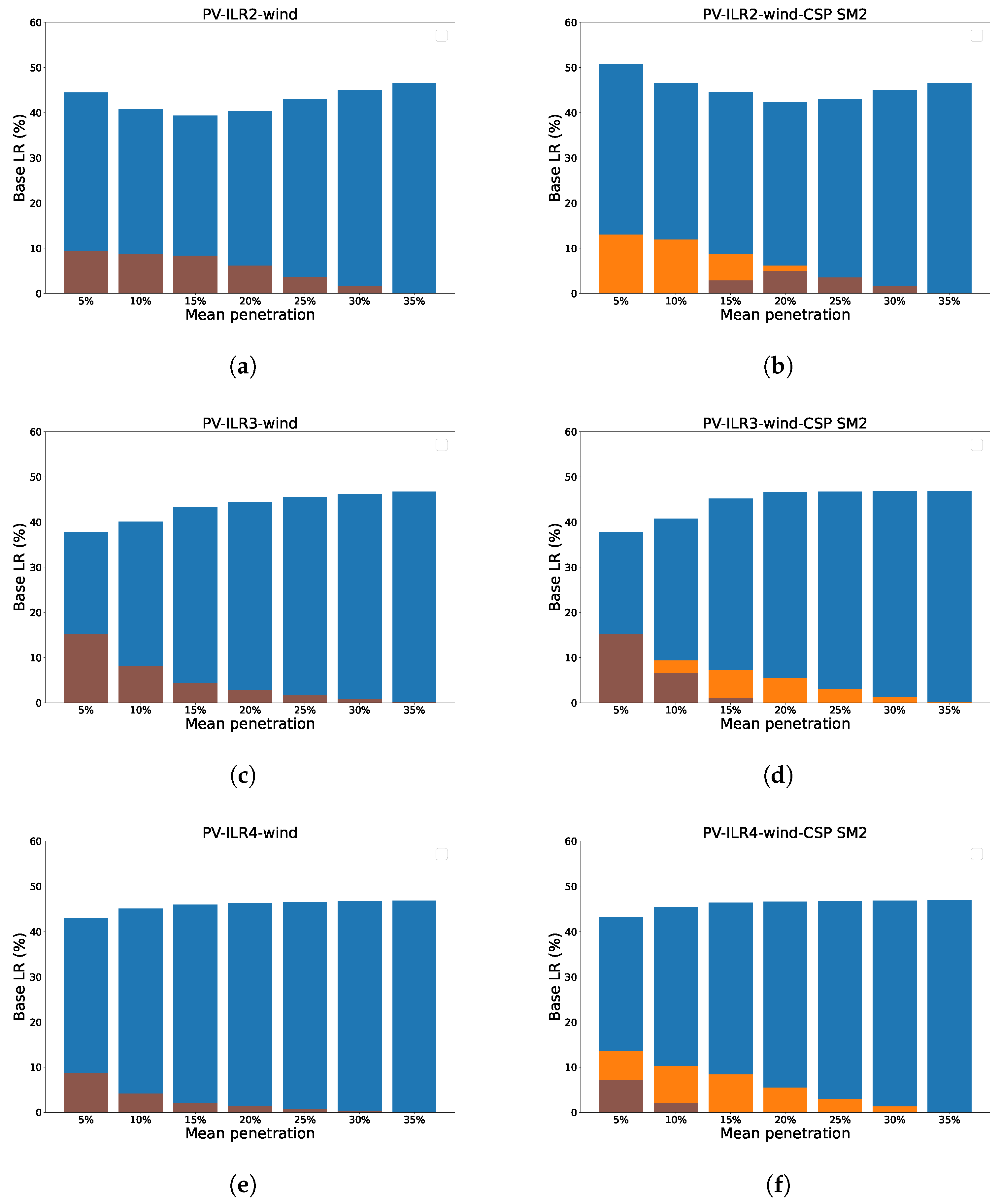
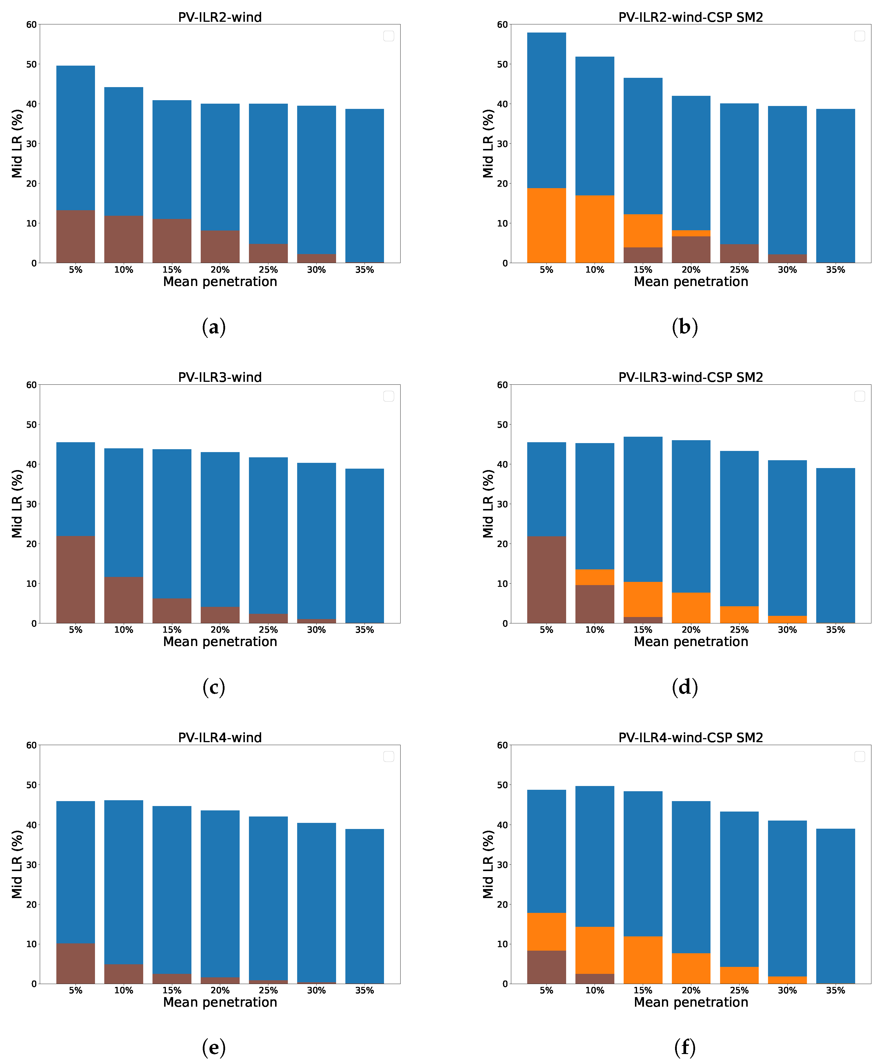
In this study, we examine how two solar technologies, Photovoltaic (PV) and Concentrated Solar Power (CSP), with different storage duration and rental costs, interact with wind in an optimal capacity mix, using recent (2013) cost data, under several scenario mixes. We analyse the role of temporal and spatial meteorological patterns, as well as the impact of Thermal Energy Storage (TES) and Battery Energy Storage (BES) associated with these solar technologies in reducing the variance-based risk. We compare the value that CSP-TES and PV-BES bring to the grid, as defined by the capacity credit, mid- and base-load reduction.

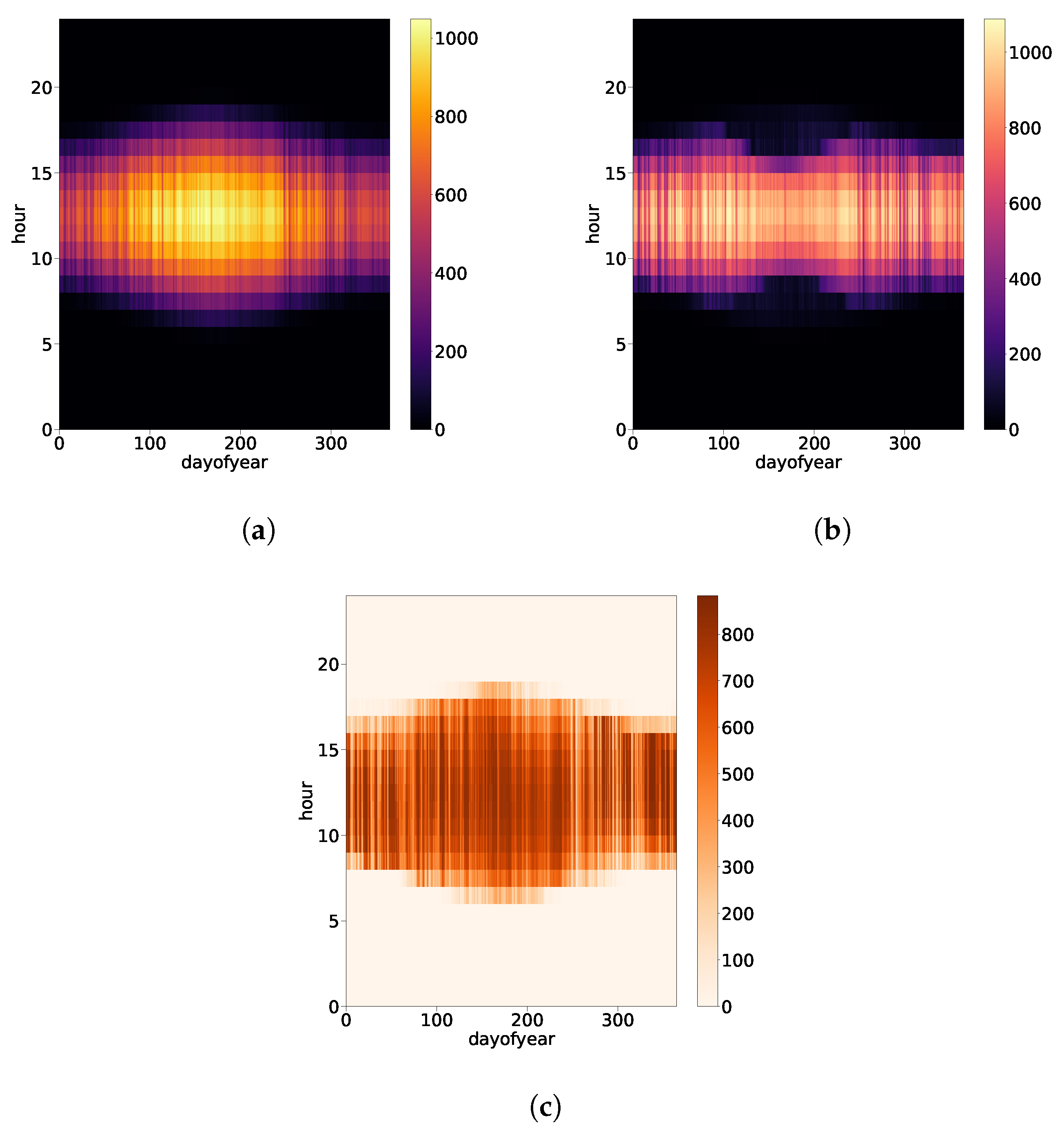
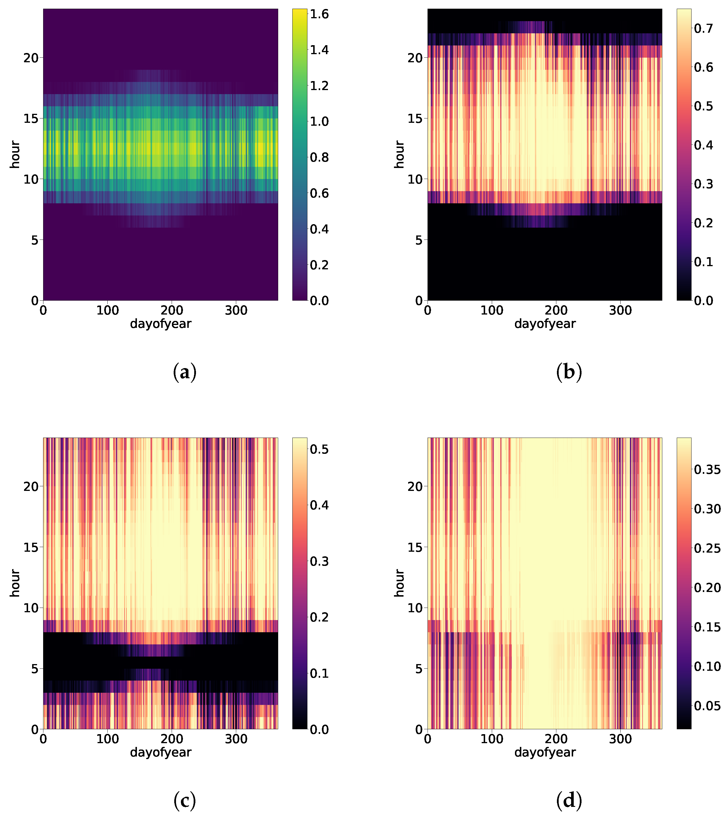
To do so, we used hourly climate data provided by MERRA-2 climate reanalysis to compute time series of demand, capacity factors (CFs) of wind, solar CSP (resp., PV) without and with increasing size of CSP solar field (resp., PV solar panel) relative to a fixed capacity of CSP power block (resp., PV inverter) capacity, as measured by the Solar Multiple SM (resp., Inverter Loading Ratio ILR). These predictions are then adjusted to energy observations for the four Moroccan electrical zones over the year 2018. For the optimal mix analysis, a Mean-Variance Portfolio approach is adopted with the objective of maximizing the renewable (RE) production and minimizing its variability while not exceeding the total cost of the actual PV-Wind-CSP-TES mix (with 5.5 h of TES). We define the rental cost of storage and generation technologies taking their dependence on the storage size into account. By diagnosing the contribution of different RE technologies to the reduction of different load bands, such as the capacity credit for the peak load, we give an analysis of the services provided by each technology.

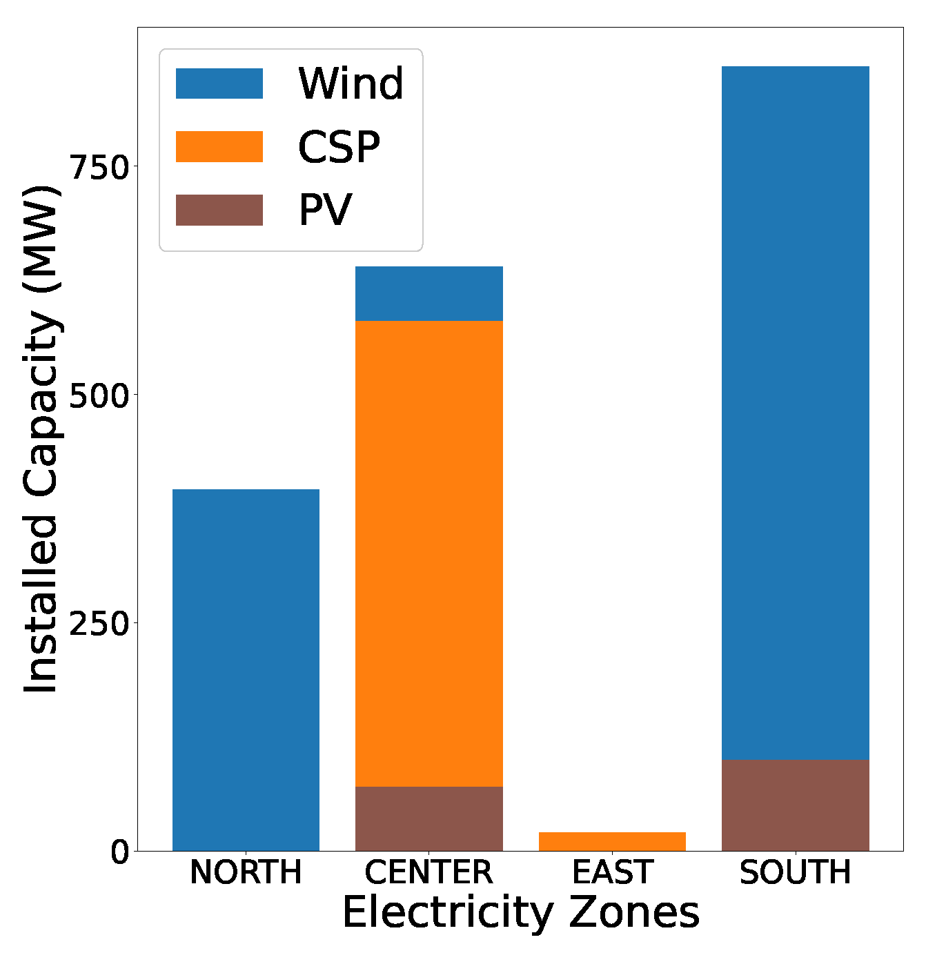
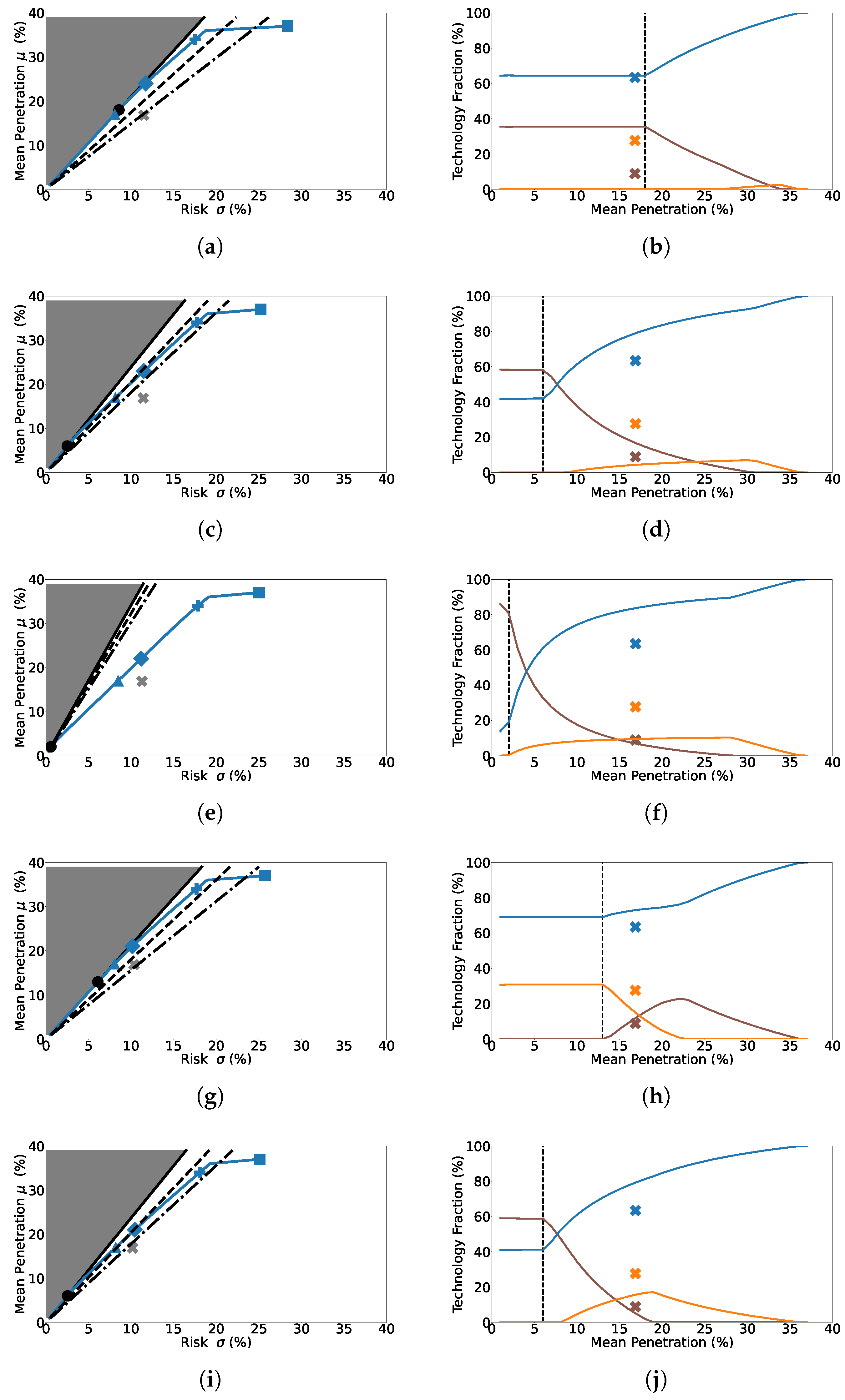
To summarize, we find that at low penetrations, the optimal mixes satisfy the maximum-cost budget without being constrained by it. More the battery storage combined with PV is large, more PV-BES in CENTER is able to meet the daily and seasonal peak demand and is winning over the low-variance wind of southern regions, while CSP capacities without storage are null. When co-locating PV-BES and CSP-TES with the same design, the latter leads to lower variability due to its larger storage capacity. If substantial BES capacity is deployed, more than that of TES, PV-BES is more likely to produce energy at minimum variance which replaces CSP-TES capacities installed in eastern or southern regions.

At high penetrations, mixes are sensitive to cost, more so as CSP and PV with high amounts of energy available for storage are introduced. Therefore, capacities are no longer linearly dependent on the mean penetration. Wind in EAST (resp., SOUTH) constitutes the predominant technology at maximum penetration mix (resp., at penetrations smaller than the maximum) presenting strong mean CF and noticeably lower rental cost while PV-BES has low mean CF and CSP/CSP-TES has high capital cost, leading to a downward trend of their fraction with increasing penetrations letting the variability increase (i.e., wind curtailment). Since costs matter at such high penetrations, the sizing of BES and TES is critical. That is, for scenarios with low–medium storage duration, ranging from 5 to 13.5 h, CSP-TES is preferred, while scenarios with longer plant operation favour PV-BES, which allows more PV-BES to be added instead to satisfy the high penetration level.

The amount of storage and the associated rental cost are thus a determinant for the technology that should be installed at low and high penetrations. It also impacts the extent to which leveraging weaker correlations between electricity zones and technologies allows for the reduction of the variability of the aggregate RE production with respect to the demand. If regional diversification and covariances between solar technologies are essential to take into account in the absence of or with small amounts of storage, the role they play in the optimization is reduced with an increase in the storage sizing, since mixes become less diversified.

While the integration of CSP/CSP-TES makes the optimal mixes sensitive to storage at low penetrations only due to the reduced variance of TES [51], the addition of BES to PV reveals an increased sensitivity of the mix to solar technologies at low and high penetrations due to the differences in the storage capacity and cost. Along the optimal fronts, we identified a highly non-linear relationship between CSP/CSP-TES and PV/PV-BES. It is noticed that when one technology is introduced in the mix, the other one is phased out and vice versa. However, in the case of unlimited PV and CSP storage capacity and ignoring storage cost, PV-BES is preferred at low and high penetrations (Figure A3) due to its low sensitivity to clouds and low rental cost compared to CSP.

These results allow us to discuss the scenarios of solar integration in Morocco. For instance, for scenarios in which Morocco aims only to reduce the risk of not covering the load, a diversified mix combining wind and PV without or with a small amount of storage or relying only on CSP-TES in its renewable goals would be efficient to reduce the foreign energy dependence. CSP without storage is sub-optimal from an economic standpoint but also cannot compete with PV because cloudy weather limits its penetration. Eventually, it should rather be viewed as an option to replace fixed-tilted PV to satisfy the demand in future warming climate where the increasing air conditioning use causes the demand to peak in summer as CSP has linear response to ambient temperature with a positive gradient [95].

Under scenarios aiming to increase the RE penetration with small RE investment—setting aside the risk related to system adequacy (i.e., curtailment or shortage situations) or in cases when Morocco relies on its current flexibility options (i.e., imports from Spain, pumped hydro storage or demand response) [96] to alleviate these issues, Morocco has to invest more in wind due to its strong and regular Cf—along the Atlas mountain ridge in eastern regions and southern regions where the coastal climate effect of the Atlantic ocean can be more intense and reliable—which could reduce the costs that an investor would face every year compared to currently expensive CSP-TES plants (consonant with [86]). Dispatchable CSP plants with high storage capacity will very likely reduce the intermittency of PV and the variability of wind feed-in at such high RE share scenarios if Morocco increased the RE budget [51]. The low PV/PV-BES mean CF resulting from the moderate PV efficiency conditions of Morocco—mainly due to its sensitivity to high temperatures [97]—is the reason why despite their rather low rental cost, only a small number of PV capacities are installed at such high penetrations. Thus, investment must be increased to use battery with large storage and/or a tracking system to achieve high-capacity credit [11].

It is important to bear in mind that in this study, PV multi-crystalline and CSP parabolic trough (PT) have been used as reference solar technologies in the PV/PV-BES and CSP/CSP-TES models. Moreover, the output is only for CSP North–South tracking and fixed latitude-tilted PV. However, care should be taken to test different technologies and tracking types since each option has its own characteristics in terms of sensitivity to temperature, cost and learning rates. For instance, the multi-crystalline PV efficiency decreases as the PV cells get hotter [98]. However, amorphous silicon solar cells are less sensitive to high temperature (0.19% vs. 0.50% degradation per degree over 25 °C) [99]. In addition, it is possible that technology innovations in the CSP sector will lead to future market preference for other CSP technologies instead of the PT, such as Solar Tower (ST). The latter has lower cost of storage and power block [49] due to the higher operating temperature, which creates a greater temperature differential and higher performance. Therefore, ST has the potential to reduce costs for providing mid and peak load in hot and arid climate, further improving their competitiveness at high penetration scenarios in Morocco. Therefore, the elicited conclusions should be treated as a revealing qualitative trend since the costs of PV, wind, CSP and batteries are expected to come down due to large-scale deployment and technology improvements [5]. Additional analyses are needed to evaluate the sensitivity of the results to alternative PV and CSP technologies, tracking types, storage configuration and cost scenarios data.

While evaluating the impact of cost and storage of PV and CSP on their integration is a first step, ultimately estimating the avoided operational costs from conventional and the revenues that may be achieved during periods of high-peak demand or high electricity prices will be important for system planners. Further refinements are thus needed to take into consideration in the optimization framework.

This modelling framework can be implemented in future warming climate to assess the impact of climate change on optimal mixes and the role of storage in reducing the Moroccan climate sensitivity.

References

1. Arroyo, R.M.; Miguel, L.J. The Role of Renewable Energies for the Sustainable Energy Governance and Environmental Policies for the Mitigation of Climate Change in Ecuador. Energies 2020, 13, 3883. [Google Scholar] [CrossRef]
2. Kalair, A.; Abas, N.; Saleem, M.; Khan, N. Role of Energy Storage Systems in Energy Transition from Fossil Fuels to Renewables. Energy Storage 2021, 3, e135. [Google Scholar] [CrossRef] [Green Version]
3. Drennen, T.; Erickson, J.; Chapman, D. Solar power and Climate Change Policy in Developing Countries. Energy Policy 1993, 24, 9–16. [Google Scholar] [CrossRef]
4. Chiaro, B.D.; Payne, S.; Dutzik, T. Solar Thermal Power and the Fight Against Global Warming; Environment America Research & Policy Center: Denver, CO, USA, 2008. [Google Scholar]
5. REN21. Renewables 2019 Global Status Report; REN21: Paris, France, 2020. [Google Scholar]
6. IEA-PVPS. Snapshot of Global PV Markets. IEA, 2020. Available online: https://iea-pvps.org/wp-content/uploads/2020/04/IEA_PVPS_Snapshot_2020.pdf (accessed on 21 June 2021).
7. Hamilton, W.T.; Husted, M.; Newman, A.; Braun, R.; Wagner, M. Dispatch Optimization of Concentrating Solar Power with Utility-Scale Photovoltaics. Optim. Eng. 2020, 21, 335–369. [Google Scholar] [CrossRef]
8. Madaeni, S.H.; Sioshansi, R.; Denholm, P. How Thermal Energy Storage Enhances the Economic Viability of Concentrating Solar Power. Proc. IEEE 2012, 100, 335–347. [Google Scholar] [CrossRef]
9. Mehos, M.; Jorgenson, J.; Denholm, P.; Turchi, C. An Assessment of the Net Value of CSP Systems Integrated with Thermal Energy Storage. Energy Procedia 2015, 69, 2060–2071. [Google Scholar] [CrossRef] [Green Version]
10. Alliance, C. The Economic and Reliability Benefits of CSP with Thermal Energy Storage: Literature Review and Research Needs. Report. CSP Alliance. 2014. Available online: http://www.inship.eu/docs/TES%204%20the_economic_and_reliability_benefits_of_csp_with_thermal_storage_2014_09_09_final.pdf (accessed on 21 June 2021).
11. Forrester, J. The Value of CSP with Thermal Energy Storage in Providing Grid Stability. Energy Procedia 2014, 49, 1632–1641. [Google Scholar] [CrossRef] [Green Version]
12. Denholm, P.; Wan, Y.; Hummon, M.; Mehos, M. Analysis of Concentrating Solar Power with Thermal Energy Storage in a California 33% Renewable Scenario; National Renewable Energy Laboratory: Golden, CO, USA, 2013.
13. IRENA. Renewable Energy Technologies: Cost Analysis Series—Solar Photovoltaics; Report; IRENA: Abu Dhabi, United Arab Emirate, 2012; Available online: https://www.irena.org/-/media/Files/IRENA/Agency/Publication/2012/RE_Technologies_Cost_Analysis-SOLAR_PV.pdf (accessed on 21 June 2021).
14. Albadi, M.H. Solar PV Power Intermittency and Its Impacts On Power Systems? An Overview. J. Eng. Res. 2019, 16, 142–150. [Google Scholar] [CrossRef] [Green Version]
15. Denholm, P.; O’Connell, M.; Brinkman, G.; Jorgenson, J. Overgeneration from Solar Energy in California: A Field Guide to the Duck Chart; Report; National Renewable Energy Laboratory: Golden, CO, USA, 2015. Available online: https://www.nrel.gov/docs/fy16osti/65023.pdf (accessed on 21 June 2021).
16. Frunt, J.; Kling, W.; Bosch, V. Classification and Quantification of Reserve Requirements for Balancing. Electr. Power Syst. Res. 2010, 80, 1528–1534. [Google Scholar] [CrossRef]
17. Sijm, J. Cost and Revenue Related Impacts of Integrating Electricity from Variable Renewable Energy into the Power System—A Review of Recent Literature; ECN-E-14-022; ECN: Petten, The Netherlands, 2014. [Google Scholar]
18. Hirth, L.; Ueckerdt, F.; Edenhofer, O. Integration Costs Revisited—An Economic Framework of Wind and Solar Variability. Renew. Energy 2014, 74, 925–939. [Google Scholar] [CrossRef]
19. Denholm, P.; Clark, K.; O’Connell, M. On the Path to SunShot. Emerging Issues and Challenges in Integrating High Levels of Solar into the Electrical Generation and Transmission System; EERE Publication and Product Library, 2016. Available online: https://www.nrel.gov/docs/fy16osti/65800.pdf (accessed on 10 June 2021).
20. Palmintier, B.; Broderick, R.; Mather, B.; Coddington, M.; Baker, K.; Ding, F.; Reno, M.; Lave, M.; Bharatkumar, A. On the Path to SunShot. Emerging Issues and Challenges in Integrating Solar with the Distribution System; National Renewable Energy Laboratory: Golden, CO, USA, 2016.
21. Jorgenson, J.; Denholm, P.; Mehos, M. Estimating the Value of Utility-Scale Solar Technologies in California under a 40% Renewable Portfolio Standard; Report Summary; National Renewable Energy Laboratory: Golden, CO, USA, 2014.
22. Jorgenson, J.; Mehos, M.; Denholm, P. Comparing the Net Cost of CSP-TES to PV Deployed with Battery Storage. AIP Conf. Proc. 2016, 1734, 080003. [Google Scholar]
23. Bowen, T.; Chernyakhovskiy, I.; Denholm, P. Grid-Scale Battery Storage: Frequently Asked Questions; National Renewable Energy Laboratory: Golden, CO, USA, 2019.
24. Weniger, J.; Tjaden, T.; Quaschning, V. Sizing of Residential PV Battery Systems. Energy Procedia 2014, 46, 78–87. [Google Scholar] [CrossRef] [Green Version]
25. Tervo, E.J.; Agbim, K.A.; DeAngelis, F.; Hernandez, J.; Kim, H.; Odukomaiya, A. An Economic Analysis of Residential Photovoltaic Systems with Lithium-Ion Battery Storage in the United States. Renew. Sustain. Energy Rev. 2018, 94, 1057–1066. [Google Scholar] [CrossRef]
26. Schram, W.; Lampropoulos, I.; Sark, W.V. Photovoltaic Systems Coupled with Batteries that are Optimally Sized for Household Self-Consumption: Assessment of Peak Shaving Potential. Appl. Energy 2018, 223, 69–81. [Google Scholar] [CrossRef]
27. Quoilin, S.; Kavvadias, K.; Mercier, A.; Pappone, I.; Zucker, A. Quantifying Self-Consumption Linked to Solar Home Battery Systems: Statistical Analysis and Economic Assessment. Appl. Energy 2016, 182, 58–67. [Google Scholar] [CrossRef]
28. Ke, B.; Ku, T.; Ke, Y.; Chuang, C.; Chen, H.Z. Sizing the Battery Energy Storage System on a University Campus With Prediction of Load and Photovoltaic Generation. IEEE Trans. Ind. Appl. 2016, 52, 1136–1147. [Google Scholar]
29. Heymans, C.; Walker, S.; Young, S.; Fowler, M. Economic Analysis of Second Use Electric Vehicle Batteries for Residential Energy Storage and Load-Levelling. Energy Policy 2014, 71, 22–30. [Google Scholar] [CrossRef]
30. Syed, M.; Morrison, G.M.; Darbyshire, J. Shared Solar and Battery Storage Configuration Effectiveness for Reducing the Grid Reliance of Apartment Complexes. Energies 2020, 13, 4820. [Google Scholar] [CrossRef]
31. Say, K.; Schill, W.; John, M. Degrees of Displacement: The Impact of Household PV Battery Prosumage on Utility Generation and Storage. arXiv 2020, arXiv:2003.0698. [Google Scholar]
32. Hassan, A.S.; Cipcigan, L.; Jenkins, N. Optimal Battery Storage Operation for PV Systems with Tariff Incentives. Appl. Energy 2017, 203, 422–441. [Google Scholar] [CrossRef]
33. Shibata, Y. How Can “Solar PV + Battery System” Be Economically Competitive Reliable Power Generation? Strategies for Post—FIT; The Institute of Electrical Engineers of Japan (IEEJ): Tokyo, Japan, July 2017.
34. Borowy, B.; Salameh, Z. Methodology for Optimally Sizing the Combination of a Battery Bank and PV Array in a Wind/PV Hybrid System. IEEE Trans. Energy Convers. 1996, 11, 367–375. [Google Scholar] [CrossRef]
35. Ashari, M.; Nayar, C. An Optimum Dispatch Strategy Using Set Points for a Photovoltaic (PV)–Diesel–Battery Hybrid Power System. Sol. Energy 1999, 66, 1–9. [Google Scholar] [CrossRef]
36. Scioletti, M.; Newman, A.; Goodman, J.K.; Zolan, A.J.; Leyffer, S. Optimal Design and Dispatch of a System of Diesel Generators, Photovoltaics and Batteries for Remote Locations. Optim. Eng. 2017, 18, 755–792. [Google Scholar] [CrossRef]
37. Gitizadeh, M.; Fakharzadegan, H. Battery Capacity Determination with Respect to Optimized Energy Dispatch Schedule in Grid-Connected Photovoltaic (PV) Systems. Energy 2014, 65, 665–674. [Google Scholar] [CrossRef]
38. Riffonneau, Y.; Bacha, S.; Barruel, F.; Ploix, S. Optimal Power Flow Management for Grid Connected PV Systems with Batteries. IEEE Trans. Sustain. Energy 2011, 2, 309–320. [Google Scholar] [CrossRef]
39. Nottrott, A.; Kleissl, J.; Washom, B. Storage Dispatch Optimization for Grid-Connected Combined Photovoltaic-Battery Storage Systems. In Proceedings of the 2012 IEEE Power and Energy Society General Meeting, San Diego, CA, USA, 22–26 July 2012; pp. 1–7. [Google Scholar]
40. Shi, J.; Lee, W.; Liu, Y.; Yang, Y.; Wang, P. Forecasting Power Output of Photovoltaic Systems Based on Weather Classification and Support Vector Machines. IEEE Trans. Ind. Appl. 2012, 48, 1064–1069. [Google Scholar] [CrossRef]
41. Nottrott, A.; Kleissl, J.; Washom, B. Energy Dispatch Schedule Optimization and Cost Benefit Analysis for Grid-Connected, Photovoltaic-Battery Storage Systems. Renew. Energy 2013, 55, 230–240. [Google Scholar] [CrossRef]
42. Lu, B.; Shahidehpour, M. Short-term Scheduling of Battery in a Grid-Connected PV/Battery System. IEEE Trans. Power Syst. 2005, 20, 1053–1061. [Google Scholar] [CrossRef]
43. Marwali, M.; Hai-li, M.; Shahidehpour, S.M.; Abdul-Rahman, K.H. Short term Generation Scheduling in Photovoltaic-Utility Grid with Battery Storage. IEEE Trans. Power Syst. 1997, 13, 1057–1062. [Google Scholar] [CrossRef]
44. Khan, M.R.B.; Pasupuleti, J.; Al-Fattah, J.; Tahmasebi, M. Energy management system for PV-Battery microgrid based on model predictive control. Indones. J. Electr. Eng. Comput. Sci. 2019, 15, 20–25. [Google Scholar] [CrossRef]
45. Fabietti, L.; Gorecki, T.T.; Namor, E.; Sossan, F.; Paolone, M.; Jones, C. Enhancing the Dispatchability of Distribution Networks through Utility-Scale Batteries and Flexible Demand. Energy Build. 2018, 172, 125–138. [Google Scholar] [CrossRef]
46. Trieb, F.; O’Sullivan, M.; Pregger, T.; Schillings, C.; Krewitt, W. Characterisation of Solar Electricity Import Corridors from MENA to Europe; German Aerospace Center (DLR), Institute of Technical Thermodynamic: Köln, Germany, 2009. [Google Scholar]
47. Moser, M.; Trieb, F.; Fichter, T. Potential of Concentrating Solar Power Plants for the Combined Production of Water and Electricity in MENA Countries. J. Sustain. Dev. Energy Water Environ. Syst. 2013, 1, 122–140. [Google Scholar] [CrossRef] [Green Version]
48. Feldman, D.; Margolis, R.; Denholm, P.; Stekli, J. Exploring the Potential Competitiveness of Utility-Scale Photovoltaics Plus Batteries with Concentrating Solar Power, 2015–2030; National Renewable Energy Laboratory: Golden, CO, USA, 2016.
49. IRENA. Renewable Energy Technologies: Cost Analysis Series—Concentrating Solar Power; Report; IRENA: Abu Dhabi, United Arab Emirate, 2012; Available online: https://www.irena.org/documentdownloads/publications/re_technologies_cost_analysis-csp.pdf (accessed on 21 June 2021).
50. Advanced CSP Teaching Materials Chapter 9 Thermal Energy Storage. Available online: https://dokumen.tips/documents/chapter-9-thermal-energy-storage-energy-09advanced-csp-teaching-materials.html (accessed on 21 June 2021).
51. Bouramdane, A.; Tantet, A.; Drobinski, P. Adequacy of Renewable Energy Mixes with Concentrated Solar Power and Photovoltaic in Morocco: Impact of Thermal Storage and Cost. Energies 2020, 13, 5087. [Google Scholar] [CrossRef]
52. Bogdanov, D.; Breyer, C. The Role of Solar Energy towards 100% Renewable Power Supply for Israel: Integrating Solar PV, Wind Energy, CSP and Storages. In Proceedings of the 19th Sede Boqer Symposium on Solar Electricity Production, Sede Boqer, Israel, 23–25 February 2015. [Google Scholar]
53. Chattopadhyay, D.; Bánkuti, M.; Bazilian, M.; de Sisternes, F.D.; Oguah, S.; Sánchez, M. Capacity Planning Model with CSP and Battery. In Proceedings of the 2018 IEEE Power & Energy Society General Meeting (PESGM), Portland, OR, USA, 5–10 August 2018; pp. 1–5. [Google Scholar]
54. Lovegrove, K.; James, G.; Leitch, D.; Milczarek, A.; Ngo, A.; Rutovitz, J.; Watt, M.; Wyder, J. Comparison of Dispatchable Renewable Electricity Options: Technologies for an Orderly Transition; ITP Thermal Pty Ltd.: Sydney, Australia, 2018. [Google Scholar]
55. Kumar, A.V.; Verma, A.; Singal, L. An Economic Examination of Solar Energy with Storage based Supply Options: Solar PV-Battery and CSP with Thermal-Storage. Int. J. Eng. Adv. Technol. (IJEAT) 2019, 8, 740–748. [Google Scholar]
56. Zurita, A.; Mata-Torres, C.; Cardemil, J.; Escobar, R. Evaluating different Operation Modes of a Hybrid CSP+PV+TES+BESS Plant Varying the Dispatch Priority. AIP Conf. Proc. 2019, 2126, 090007. [Google Scholar]
57. Papadopoulou, A.; Vasileiou, G.; Flamos, A. A Comparison of Dispatchable RES Technoeconomics: Is There a Niche for Concentrated Solar Power? Energies 2020, 13, 4768. [Google Scholar] [CrossRef]
58. Poullikkas, A. A Comparative Overview of Large-Scale Battery Systems for Electricity Storage. Renew. Sustain. Energy Rev. 2013, 27, 778–788. [Google Scholar] [CrossRef]
59. IRENA. Utility-Scale Batteries Innovation Landscape Brief; Report; IRENA: Abu Dhabi, United Arab Emirate, 2019; Available online: https://www.irena.org/-/media/Files/IRENA/Agency/Publication/2019/Sep/IRENA_Utility-scale-batteries_2019.pdf (accessed on 21 June 2021).
60. Denholm, P.; Mehos, M. Enabling Greater Penetration of Solar Power via the Use of CSP with Thermal Energy Storage; National Renewable Energy Laboratory: Golden, CO, USA, 2011. [CrossRef] [Green Version]
61. Narimani, A.; Abeygunawardana, A.; Nourbakhsh, G.; Ledwich, G.; Walker, G. Comparing Operational Value of CSP with TES to PV with Battery Storage in Australian National Electricity Market. In Proceedings of the 2017 Australasian Universities Power Engineering Conference (AUPEC), Melbourne, Australia, 19–22 November 2017; pp. 1–5. [Google Scholar]
62. Mills, A. An Evaluation of Solar Valuation Methods Used in Utility Planning and Procurement Processes; Lawrence Berkeley National Laboratory: Berkeley, CA, USA, 2014.
63. Denholm, P.; Margolis, R.; Eichman, J.D. Evaluating the Technical and Economic Performance of PV Plus Storage Power Plants; Report Summary; National Renewable Energy Laboratory: Golden, CO, USA, 2017.
64. Ouammi, A.; Zejli, D.; Dagdougui, H.; Benchrifa, R. Artificial Neural Network Analysis of Moroccan Solar Potential. Renew. Sustain. Energy Rev. 2012, 16, 4876–4889. [Google Scholar] [CrossRef]
65. Joskow, P. Comparing the Costs of Intermittent and Dispatchable Electricity Generating Technologies. Am. Econ. Rev. 2011, 101, 238–241. [Google Scholar] [CrossRef] [Green Version]
66. Markowitz, H. Portfolio Selection. J. Financ. 1952, 7, 77–91. [Google Scholar]
67. Tantet, A.; Stéfanon, M.; Drobinski, P.; Badosa, J.; Concettini, S.; Créti, A.; D’Ambrosio, C.; Thomopulos, D.; Tankov, P. E4clim 1.0: The Energy for a Climate Integrated Model: Description and Application to Italy. Energies 2019, 12, 4299. [Google Scholar] [CrossRef] [Green Version]
68. Ministère de l’Energie, des Mines et de l’Environnement (MEME). Available online: https://www.mem.gov.ma/pages/index.aspx (accessed on 21 June 2021).
69. Gami, D.; Sioshansi, R.; Denholm, P. Data Challenges in Estimating the Capacity Value of Solar Photovoltaics. IEEE J. Photovolt. 2017, 7, 1065–1073. [Google Scholar] [CrossRef]
70. Gelaro, R.; McCarty, W.; Suárez, M.; Todling, R.; Molod, A.; Takacs, L.L.; Randles, C.; Darmenov, A.; Bosilovich, M.; Reichle, R.; et al. The Modern-Era Retrospective Analysis for Research and Applications, Version 2 (MERRA-2). J. Clim. 2017, 30, 5419–5454. [Google Scholar] [CrossRef]
71. Khatib, N. Country Profile Morocco. Report. RES4MED&Africa. 2018. Available online: https://www.res4africa.org/wp-content/uploads/2018/06/Country-profile-Marocco-2.pdf (accessed on 21 June 2021).
72. Solar Power and Chemical Energy Systems (SolarPACES). Available online: https://solarpaces.nrel.gov/ (accessed on 21 June 2021).
73. CSP Focus. Available online: http://www.cspfocus.cn/en/ (accessed on 21 June 2021).
74. Duffie, J.A.; Beckman, W.A. Solar Engineering of Thermal Processes, 4th ed.; Wiley: New York, NY, USA, 2013; 944p. [Google Scholar]
75. Stine, W.B.; Geyer, M. Power From The Sun, 4th ed.; 2001; Available online: https://www.powerfromthesun.net/book.html (accessed on 29 July 2021).
76. Patnode, A. Simulation and Performance Evaluation of Parabolic Trough Solar Power Plants. Ph.D. Thesis, University of Wisconsin-Madison, Madison, WI, USA, 2006. Available online: http://digital.library.wisc.edu/1793/7590 (accessed on 21 June 2021).
77. Hosenuzzaman, M.; Rahim, N.A.; Selvaraj, J.; Hasanuzzaman, M.; Malek, A.A.; Nahar, A. Global Prospects, Progress, Policies, and Environmental Impact of Solar Photovoltaic Power Generation. Renew. Sustain. Energy Rev. 2015, 41, 284–297. [Google Scholar] [CrossRef]
78. Lumby, B.; Miller, A. Utility Scale Solar Power Plants: A Guide for Developers and Investors; World Bank Group: New Delhi, India, 2012. [Google Scholar]
79. Bousselamti, L.; Cherkaoui, M. Modelling and Assessing the Performance of Hybrid PV-CSP Plants in Morocco: A Parametric Study. Int. J. Photoenergy 2019, 2019, 1–15. [Google Scholar] [CrossRef] [Green Version]
80. Guédez, R.; Spelling, J.; Laumert, B.; Fransson, T. Optimization of Thermal Energy Storage Integration Strategies for Peak Power Production by Concentrating Solar Power Plants. Energy Procedia 2014, 49, 1642–1651. [Google Scholar] [CrossRef] [Green Version]
81. According to Abdelkader Himdi, Director of Operations and Maintenance at MASEN and Sergio Relloso, Performance Guarantee Manager at SENER, EPC Partner to All Three Phases of the Ouarzazate Project. Available online: https://www.solarpaces.org/csp-puts-end-morocco-electricity-blackouts/ (accessed on 29 July 2021).
82. Cretì, A.; Fontini, F. Economics of Electricity: Markets, Competition and Rules; Cambridge University Press: Cambridge, UK, 2019; p. 214. [Google Scholar] [CrossRef]
83. Ioannis, T.; Dalius, T.; Andreas, Z. Cost Development of Low Carbon Energy Technologies—Scenario-based Cost Trajectories to 2050, 2017 Edition; EUR 29034 EN; Publications Office of the European Union: Luxembourg, 2018. [Google Scholar] [CrossRef]
84. Advanced CSP Teaching Materials Chapter 5 Parabolic Trough Technology. Available online: https://fdocuments.in/document/chapter-5-parabolic-trough-technology.html (accessed on 21 June 2021).
85. Richts, C. The Moroccan Solar Plan: A Comparative Analysis of CSP and PV Utilization Until 2020. Master’s Thesis, University of Kassel, Kassel, Germany, 2012. Available online: https://inis.iaea.org/search/search.aspx?orig_q=RN:47087488 (accessed on 21 June 2021).
86. Brand, B.; Stambouli, A.B.; Zejli, D. The Value of Dispatchability of CSP Plants in the Electricity Systems of Morocco and Algeria. Energy Policy 2012, 47, 321–331. [Google Scholar] [CrossRef] [Green Version]
87. Alhamwi, A.; Kleinhans, D.; Weitemeyer, S.; Vogt, T. Moroccan National Energy Strategy Reviewed From a Meteorological Perspective. Energy Strategy Rev. 2015, 6, 39–47. [Google Scholar] [CrossRef]
88. Alternative Energy from Solar, Wind, Biomass, Fuel Cells and More: PV with Batteries: A Threat to CSP? Available online: https://www.altenergymag.com/article/2014/09/pv-with-batteries-a-threat-to-csp/1500 (accessed on 29 July 2021).
89. Shirizadeh, B.; Perrier, Q.; Quirion, P. How Sensitive Are Optimal Fully Renewable Power Systems to Technology Cost Uncertainty? FAERE Policy Paper; CIRED: Paris, France, 2019; Available online: http://faere.fr/pub/PolicyPapers/Shirizadeh_Perrier_Quirion_FAERE_PP2019_04.pdf (accessed on 21 June 2021).
90. Meier, P.; Vagliasindi, M.; Imran, M. The Design and Sustainability of Renewable Energy Incentive: An Economic Analysis; Report; World Bank: Washington, DC, USA, 2015; Available online: http://hdl.handle.net/10986/20524 (accessed on 21 June 2021).
91. Roberto, L.A.; Arnulf, J.W.; Marika, V.; Bergur, S.; Davide, M.; Mindaugas, J.; Mar, P.F.M.D.; Stavros, L.; Jacopo, G.; Eveline, W.R.; et al. ETRI 2014—Energy Technology Reference Indicator Projections for 2010–2050; Joint Research Centre (JRC), European Commission (EC): Brussels, Belgium, 2014. [Google Scholar]
92. Denholm, P.; Novacheck, J.; Jorgenson, J.; O’Connell, M. Impact of Flexibility Options on Grid Economic Carrying Capacity of Solar and Wind: Three Case Studies; National Renewable Energy Laboratory: Golden, CO, USA, 2016.
93. Zhao, H.; Wu, Q.; Hu, S.; Xu, H.; Rasmussen, C. Review of Energy Storage System for Wind Power Integration Support. Appl. Energy 2015, 137, 545–553. [Google Scholar] [CrossRef]
94. Mohamed, A.; Aboubakr, E.; MOUSSAOUI, H.; El Markhi, H. Renewable Energy Potential and Available Capacity for Wind and Solar Power in Morocco Towards 2030. J. Eng. Sci. Technol. Rev. 2018, 11, 189–198. [Google Scholar] [CrossRef]
95. Crook, J.; Jones, L.A.; Forster, P.; Crook, R. Climate Change Impacts on Future Photovoltaic and Concentrated Solar Power Energy Output. Energy Environ. Sci. 2011, 4, 3101–3109. [Google Scholar] [CrossRef]
96. Boulakhbar, M.; Lebrouhi, B.; Kousksou, T.; Smouh, S.; Jamil, A.; Maaroufi, M.; Zazi, M. Towards a Large-Scale Integration of REnewable Energies in Morocco. J. Energy Storage 2020, 32, 101806. [Google Scholar] [CrossRef] [PubMed]
97. Fesharaki, V.J.; Dehghani, M.; Fesharaki, J.J. The Effect of Temperature on Photovoltaic Cell Efficiency. In Proceedings of the 1st International Conference on Emerging Trends in Energy Conservation (ETEC), Tehran, Iran, 20–21 November 2011. [Google Scholar]
98. Radziemska, E. The Effect of Temperature on the Power Drop in Crystalline Silicon Solar Cells. Renew. Energy 2003, 28, 1–12. [Google Scholar] [CrossRef]
99. PowerFilm Solar—Thin Film. Available online: https://www.powerfilmsolar.com/technology/thin-film/ (accessed on 21 June 2021).
100. Dubey, S.; Sarvaiya, J.; Seshadri, B. Temperature Dependent Photovoltaic (PV) Efficiency and Its Effect on PV Production in the World—A Review. Energy Procedia 2013, 33, 311–321. [Google Scholar] [CrossRef] [Green Version]
101. Notton, G.; Cristofari, C.; Mattei, M.; Poggi, P. Modelling of a Double-Glass Photovoltaic Module using Finite Differences. Appl. Therm. Eng. 2005, 25, 2854–2877. [Google Scholar] [CrossRef]
102. Evans, D. Simplified Method for Predicting Photovoltaic Array Output. Sol. Energy 1980, 27, 555–560. [Google Scholar] [CrossRef]
103. Reindl, D.T.; Beckman, W.; Duffie, J. Diffuse fraction Correlations. Sol. Energy 1990, 45, 1–7. [Google Scholar] [CrossRef]
104. Reindl, D.T.; Beckman, W.; Duffie, J. Evaluation of Hourly Tilted Surface Radiation Models. Sol. Energy 1990, 45, 9–17. [Google Scholar] [CrossRef]
105. Madeti, S.R.; Singh, S. A Comprehensive Study on Different Types of Faults and Detection Techniques for Solar Photovoltaic System. Sol. Energy 2017, 158, 161–185. [Google Scholar] [CrossRef]
106. Sarniak, M. Researches of the Impact of the Nominal Power Ratio and Environmental Conditions on the Efficiency of the Photovoltaic System: A Case Study for Poland in Central Europe. Sustainability 2020, 12, 6162. [Google Scholar] [CrossRef]
107. Gil, A.; Medrano, M.; Martorell, I.; Lázaro, A.; Dolado, P.; Zalba, B.; Cabeza, L. State of the Art on High Temperature Thermal Energy Storage For Power Generation. Part 1—Concepts, Materials and Modellization. Renew. Sustain. Energy Rev. 2010, 14, 31–55. [Google Scholar] [CrossRef]
108. Middle East and North Africa Concentrating Solar Power Knowledge and Innovation Program (MENA CSP KIP). Available online: http://cmimarseille.org/menacspkip/wp-content/uploads/2017/08/Youssef_Stitou_MENA_CSP_KIP_Jordan_Workshop_25_July_2017.pdf (accessed on 21 June 2021).
109. Ain Beni Mathar: Une Centrale Électrique Thermo Solaire Unique au Maroc. Available online: https://www.afdb.org/fr/projects-and-operations/selected-projects/ain-beni-mathar-aunique-thermo-solar-powerplant-in-morocco-142 (accessed on 21 June 2021).
Figure 1. Flow chart of E4CLIM components (dark blue) including the modules added (light blue) and the data sources (gray) illustrating the general framework of this study. TheE4CLIM’s flow is divided in three steps: (1) Capacity factors and demand time series are first estimated from climate grid points and fitted to observations; (2) The mix is then optimized using the Mean-Variance Portfolio (MVP) approach; (3) The mix properties (technological and geographical distribution) are analysed; (4) The load-bands reduction diagnostics based on the “Residual Load Duration Curve (RLDC)” are finally computed to give a more detailed analysis of the services provided by different RE systems.
Energies 14 04675 g001
Figure 2. (Left) Scheme of the three modules of CSP (resp., PV) plant: X = { S F , S P } ; Y = { P B , I N V } ; Θ = { T E S , B E S } ; x = { t h e r m , D C } ; and y = { e l e c } . The black arrows represent the energy flows: Solar Field (resp., Solar Panel) energy ( P X , x S M / I L R ), Energy from Solar Field (resp., Solar Panel) to Power Block (resp., Inverter) ( P X Y , x S M / I L R ), Energy stored ( P X Θ , x S M / I L R ), Energy discharged ( P Θ Y , x S M / I L R ) and total available energy injected to the Power Block (resp., Inverter) ( P X Y , x S M / I L R + P Θ Y , x S M / I L R ) and the State of charge ( S O C E , Θ S M / I L R ). (Right) Illustration of CSP (resp., PV) plant configuration with different Solar Multiple SM (resp., Inverter Loading Ratio ILR). ILR1 or SM1: without storage; ILR > 1 or SM > 1: with increasing levels of storage. See [51], Section 2.3.3, for further description of these parameters. Source: Own elaboration based on [84].
Energies 14 04675 g002
Figure 3. Storage algorithm illustrating the dispatch conditions of CSP thermal (resp., PV Direct Current—DC) energy with constraints on the storage capacity and the maximum power of charging or discharging. X = { S F , S P } ; Y = { P B , I N V } ; Θ = { T E S , B E S } ; x = { t h e r m , D C } ; and y = { e l e c } . Source: Own elaboration based on [27,85].
Energies 14 04675 g003
Figure 4. (Left) Approximations of the optimal fronts with the risk, σsglobal/technology/base, in abscissa and the mean penetration (1), μ, in ordinate. White (resp., gray) areas to the right (resp., left) are not Pareto optimal (resp., not feasible). Particularmixes are depicted: the “2018 actual solar-windmix” (gray cross); the “penetration-as-actual mix” (blue triangle) with lower risk; the “risk-as-actual mix” (blue diamond) with higher penetration; the “cost activation mix” (black dot) with the largest penetration for which themaximum-cost constraint is not active; the “cost-activatedmix” (blue plus) withmoderate penetration compared to the “maximum-penetration mix” (blue square), in which the cost constraint is activated; (Right) Shares of wind (blue line), PV-BES (brown line) and CSP/CSP-TES (orange line) capacities versus the mean penetration for the global strategy with maximum-cost constraint (5). The crosses represent the shares for the actual mix. (a,b) PV-ILR2-Wind-CSP-SM1; (c,d) PV-ILR3-Wind-CSPSM1; (e,f) PV-ILR4-Wind-CSP-SM1; (g,h) PV-ILR2-Wind-CSP-TES SM2; (i,j) PV-ILR3-Wind-CSP-TES SM2.
Energies 14 04675 g004
Figure 5. Similar to Figure 4. (a,b) PV-ILR4-Wind-CSP-TES SM2; (c,d) PV-ILR4-Wind-CSP-TES SM3; (e,f) PV-ILR2-Wind-CSP-TES SM4; (g,h) PV-ILR3-Wind-CSP-TES SM4; (i,j) PV-ILR4-Wind-CSP-TES SM4.
Energies 14 04675 g005
Figure 6. Heatmap of the national daily (ordinate) and seasonal (abscissa) variability of the solar radiation in (W/m2): Global Horizontal Irradiation (GHI) (a), Global Tilted Irradiation (GTI) (b) (to be compared with Figure 7a–d, Direct Normal Irradiation (DNI) (c) (to be compared with Figure 8). The variation over time is shown in colour by intensity in the colour bar.
Energies 14 04675 g006
Figure 7. Heatmap of the national daily (ordinate) and seasonal (abscissa) variability of the predicted capacity factors and demand (MW): PV without storage (ILR1) (a), PV-BES ILR2 (b), PV-BES ILR3 (c), PV-BES ILR4 (d), Wind (e), Demand (f). ILR > 1: with increasing levels of storage. The variation over time is shown in colour by intensity in the colour bar.
Energies 14 04675 g007
Figure 8. Heatmap of the national daily (ordinate) and seasonal (abscissa) variability of the predicted capacity factors of CSP without storage (SM1) (a), CSP-TES SM2 (b), CSP-TES SM3 (c), CSP-TES SM4 (d). SM > 1: with increasing levels of storage. The variation over time is shown in colour by intensity in the colour bar.
Energies 14 04675 g008
Figure 9. Capacity credit by each technology—Wind (blue), PV-BES (brown) and CSP-TES (orange)—versus the mean penetration (1), μ, for the global strategy (2) with maximum-cost constraint (5). (Left) PV-BES-wind mix; (Right) PV-BES-wind-CSP-TES SM2 mix. (Top) ILR2; (Middle) ILR3; (Bottom) ILR4.
Energies 14 04675 g009
Figure 10. Mid load reduction by each technology—Wind (blue), PV-BES (brown) and CSP-TES (orange)—versus the mean penetration (1), μ, for the global strategy (2) with maximum-cost constraint (5). (Left) PV-BES-wind mix; (Right) PV-BES-wind-CSP-TES SM2 mix. (Top) ILR2; (Middle) ILR3; (Bottom) ILR4.
Energies 14 04675 g010
Figure 11. Base load reduction by each technology—Wind (blue), PV-BES (brown) and CSP-TES (orange)—versus the mean penetration (1), μ, for the global strategy (2) with maximum-cost constraint (5). (Left) PV-BES-wind mix; (Right) PV-BES-wind-CSP-TES SM2 mix. (Top) ILR2; (Middle) ILR3; (Bottom) ILR4.
Energies 14 04675 g011
Figure 12. (a) RLDC for different penetrations illustrating the variation of the RLDC parameters (peak, mid and base load) with increasing penetrations and the renewable share threshold at which curtailment occurs for PV–wind–CSP-TES SM2 combination. (b) LDC and RLDC for different combinations, computed at 20% penetration (risk-as-actual mix) for the global strategy (2) with maximum-cost constraint (5), illustrating the system flexibility provided by CSP-TES.
Energies 14 04675 g012