
Nonlinear Optimal-Based Vibration Control of a Wind Turbine Tower Using Hybrid vs. Magnetorheological Tuned Vibration Absorber


Abstract
:1. Introduction
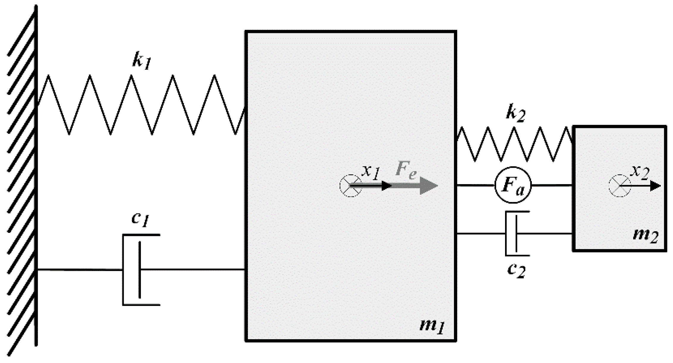
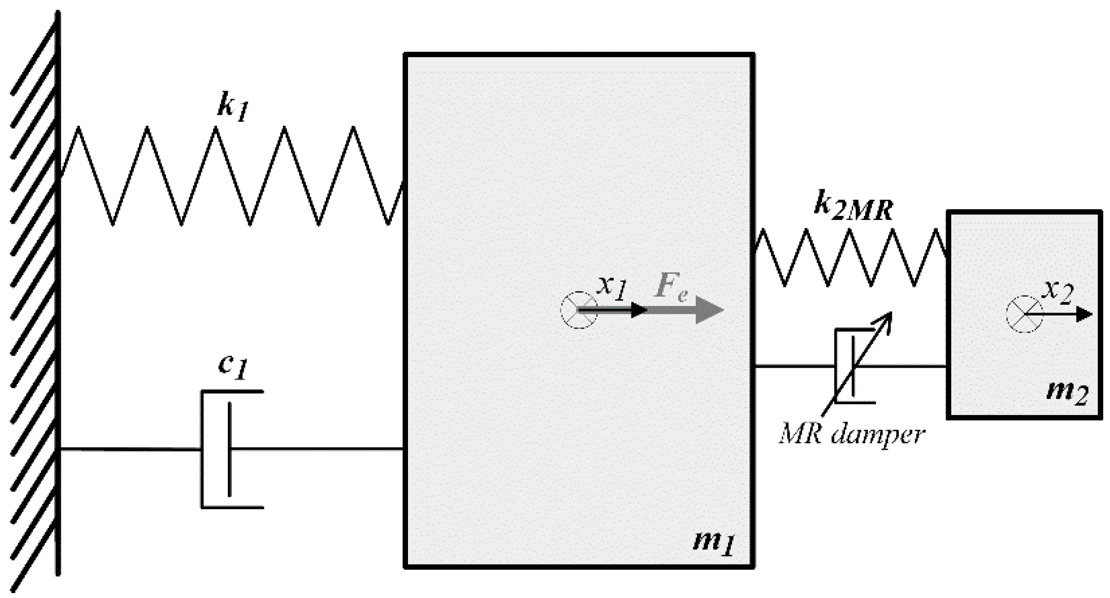
2. NREL 5.0 MW Tower-Nacelle Model with HTVA
3. Optimal Control Problem Formulation and Solution
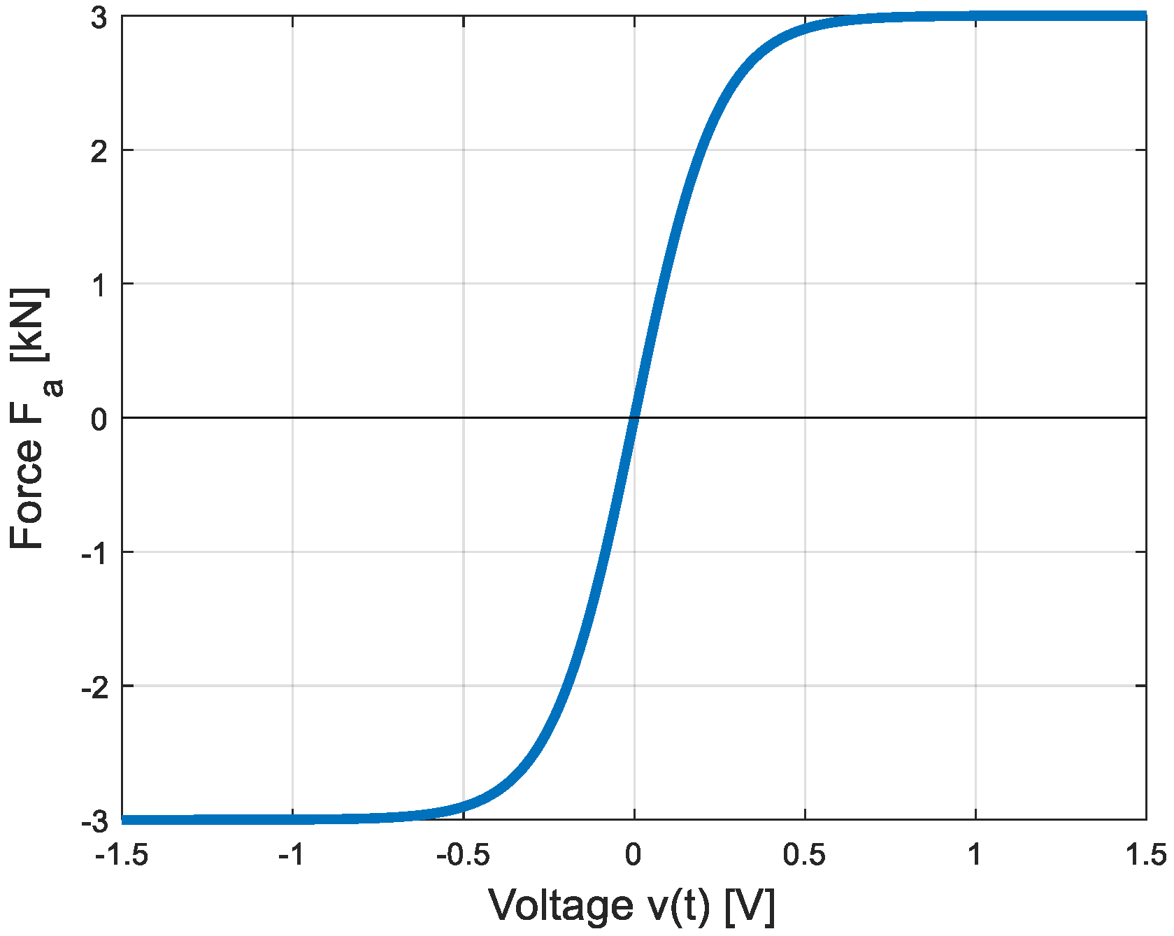
- an actuator input voltage constrained to V range,
- an unconstrained control signal , ,
- an actuator force ; thus: (see Table 1, ; note that with roundoff error below 10—5).
- 1.
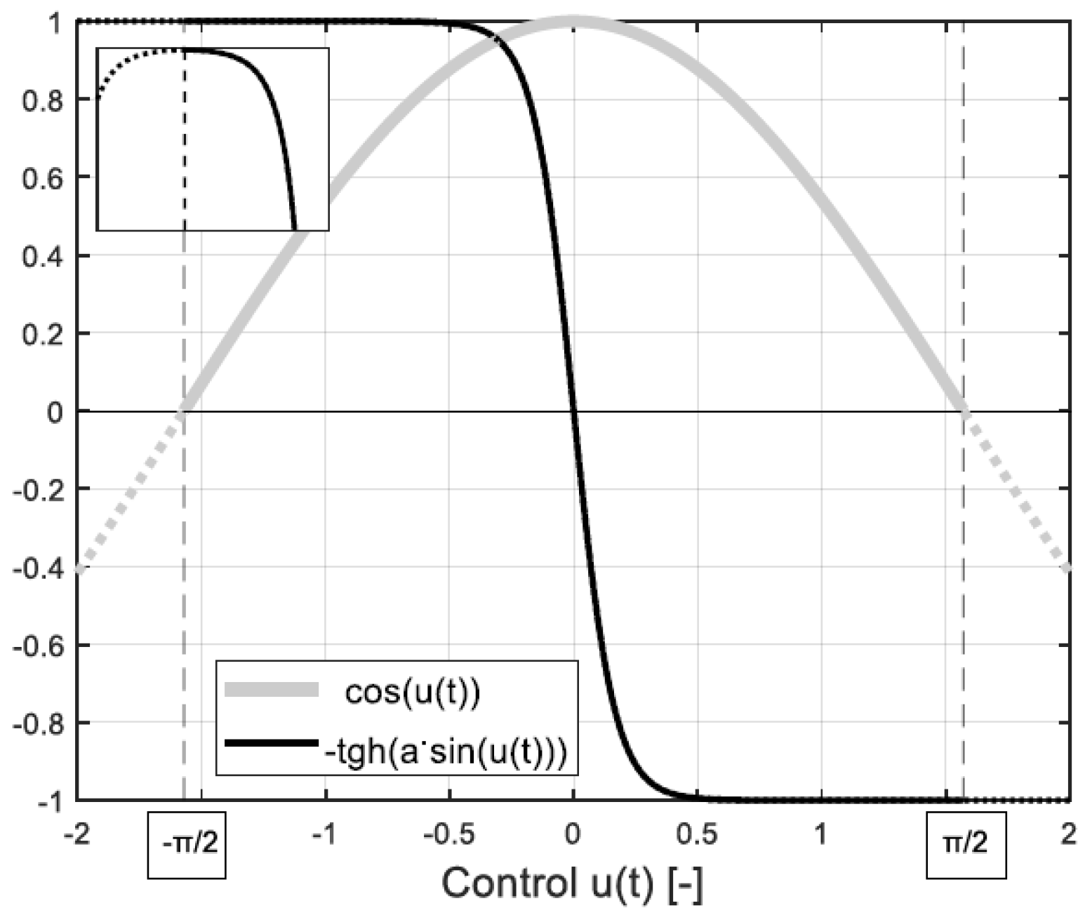
- then (14) is fulfilled and exhibits sign change (Hamiltonian maximisation) for: only, so:
- 2.
- then (14) is fulfilled and exhibits sign change for: only, so:
- 3.
- then (14) is fulfilled and exhibits sign change for: only, so:
4. Implementation Techniques
4.1. Optimal-Based Control
4.2. Hybrid Ground-Hook Control
5. Test Configurations
5.1. Optimal-Based Control for the Wind Turbine Tower-Nacelle Model with HTVA
5.2. Optimal-Based Control for the Wind Turbine Tower-Nacelle Model with MRTVA
5.3. Test Conditions
- minimisation of the primary structure deflection (nacelle-assembly displacement) amplitude as the sole objective: , , (additionally, was regarded);
- minimisation of the primary structure deflection amplitude, considering lower (than for conf. I) deflection amplitude weight with regard to actuator force weight: , , ;
- minimisation of the primary structure deflection amplitude, along with the actuator mean power: (structure deflection vs. actuator force consideration as for conf. II), , , or .
- IV.
- minimisation of the primary structure deflection (nacelle-assembly displacement) amplitude as the sole objective: , , ;
- V.
- minimisation of the primary structure deflection amplitude along with the MR damper force: , , , or .
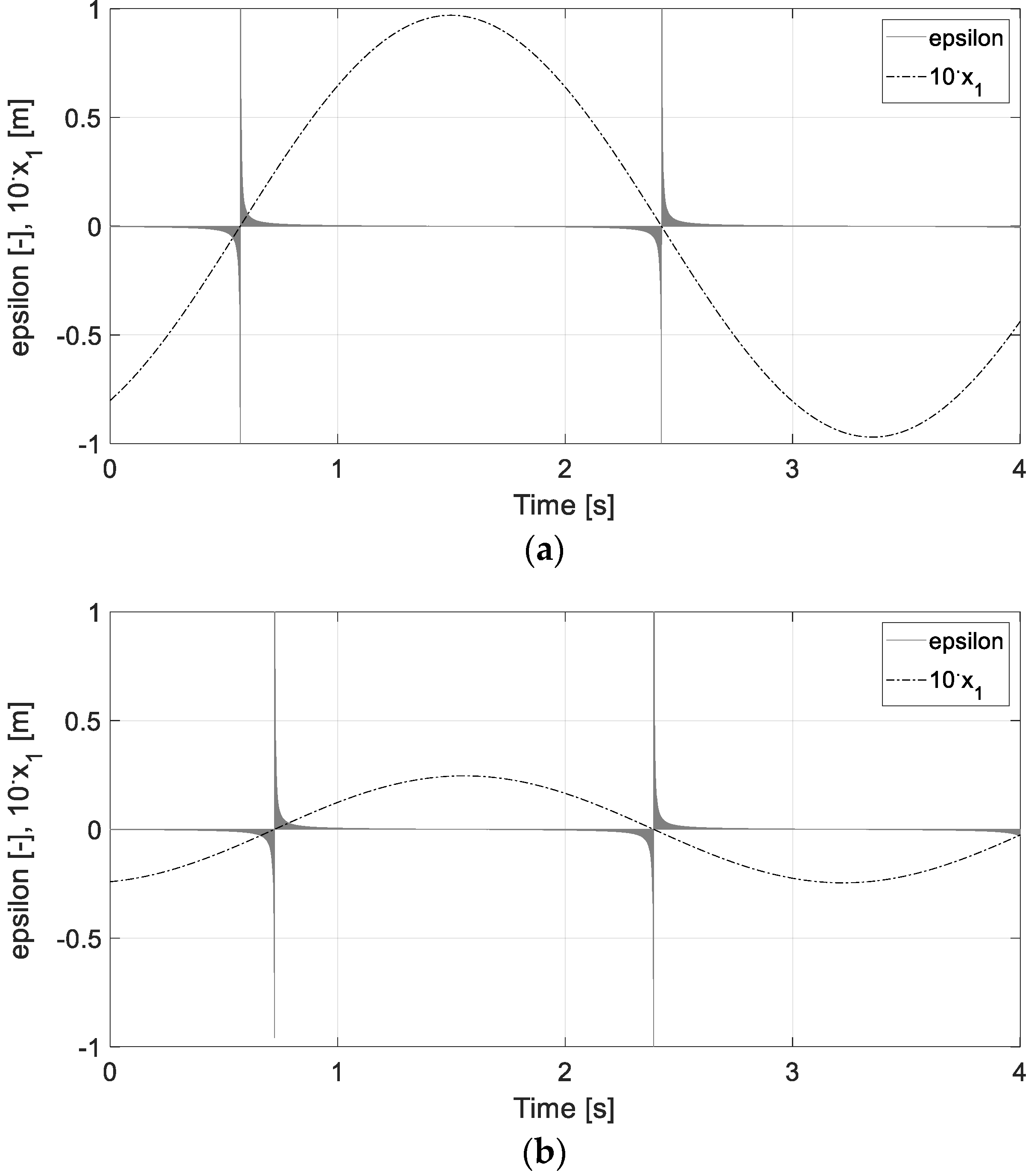
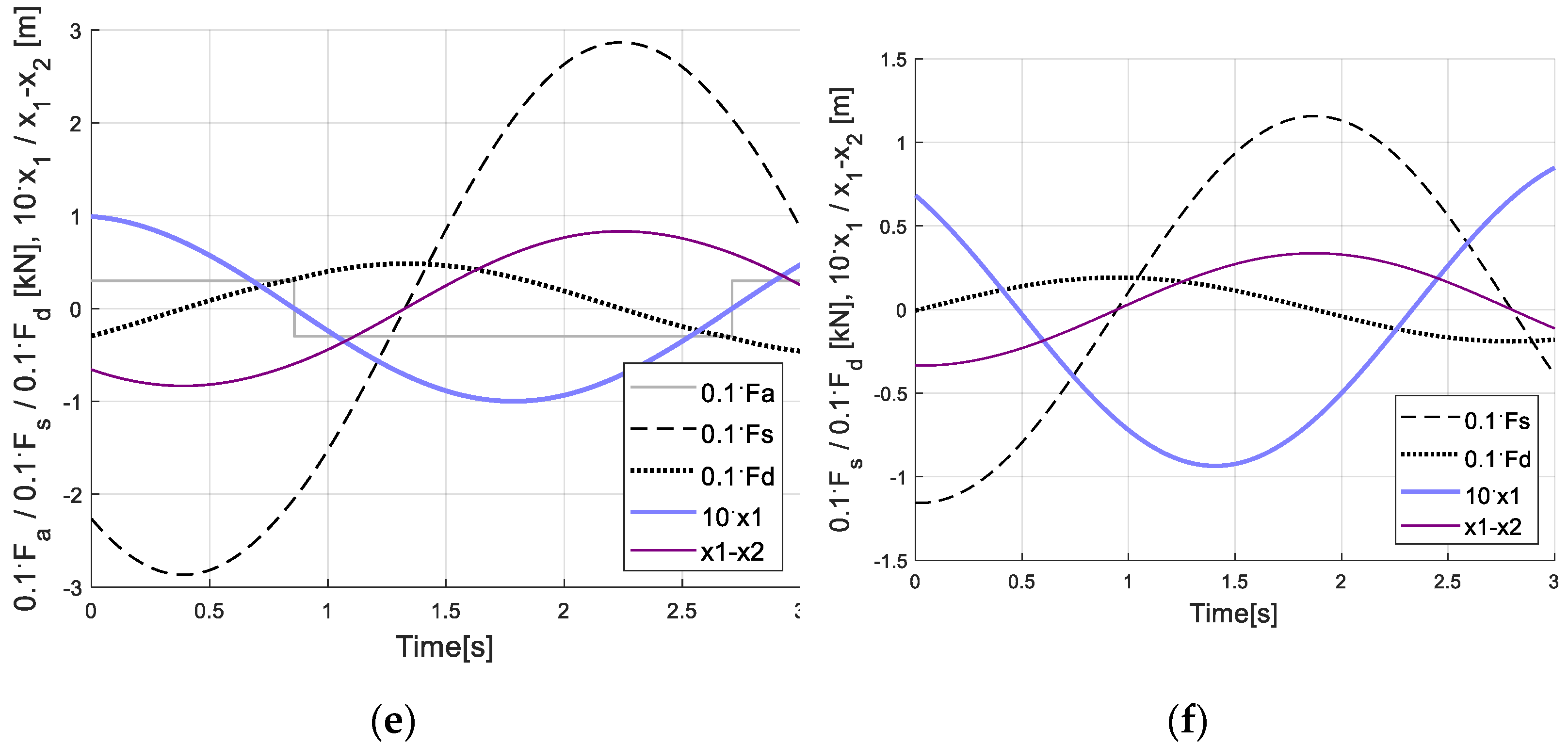
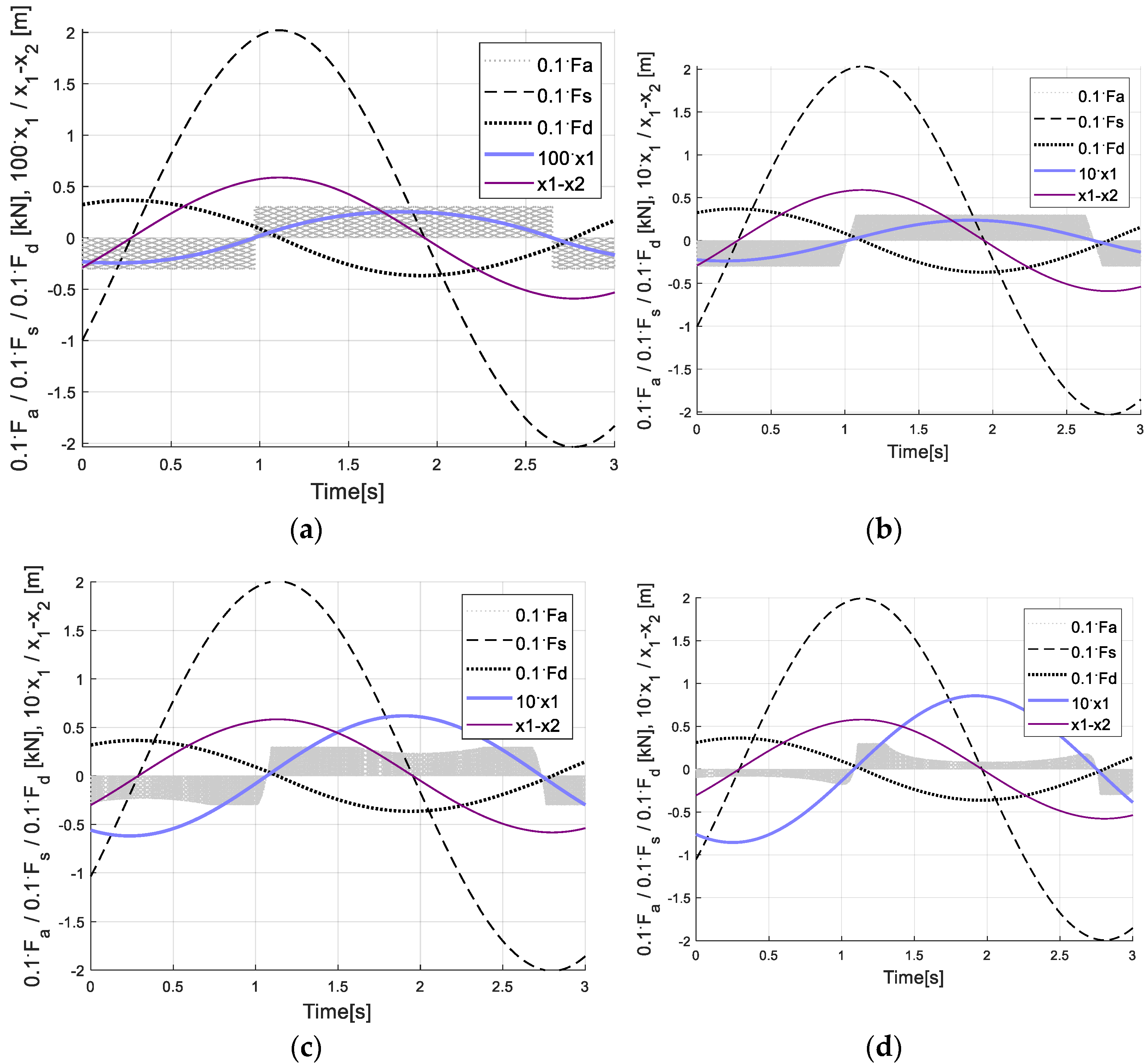
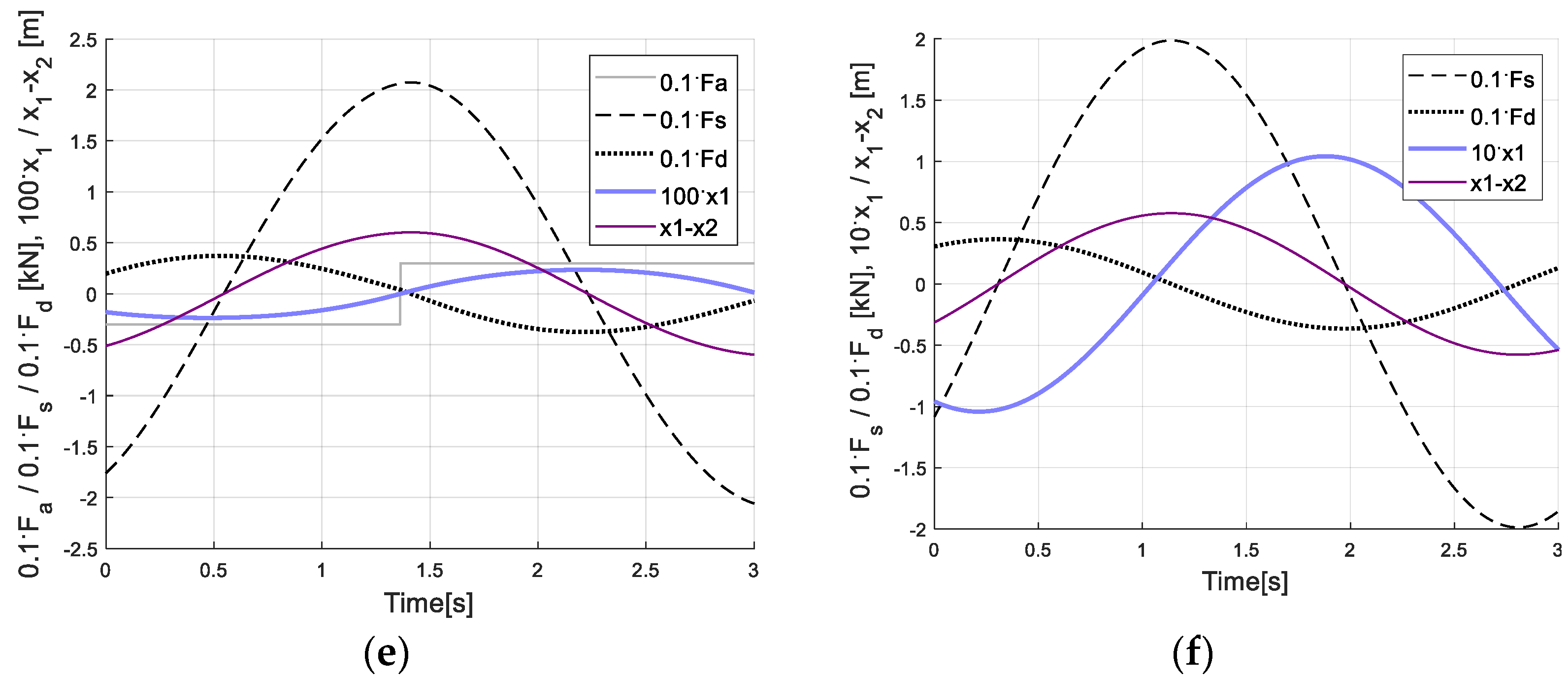
6. Control Results and Discussion
7. Conclusions
Funding
Conflicts of Interest
References
- Xu, Z.-D.; Zhu, J.-T.; Wang, D.-X. Analysis and Optimisation of Wind-Induced Vibration Control for High-Rise Chimney Structures. Int. J. Acoust. Vib. 2014, 19. [Google Scholar] [CrossRef]
- Wang, X.; Gordaninejad, F. Lyapunov-Based Control of a Bridge Using Magneto-rheological Fluid Dampers. J. Intell. Mater. Syst. Struct. 2002, 13, 7–8. [Google Scholar] [CrossRef]
- Weber, F.; Maslanka, M. Precise stiffness and damping emulation with MR dampers and its application to semi-active tuned mass dampers of Wolgograd Bridge. Smart Mater. Struct. 2014, 23, 15019. [Google Scholar] [CrossRef]
- Bakhtiari-Nejad, F.; Meidan-Sharafi, M. Vibration Optimal Control of a Smart Plate with Input Voltage Constraint of Piezoelectric Actuators. J. Vib. Control 2004, 10, 1749–1774. [Google Scholar] [CrossRef]
- Ali, S.F.; Ramaswamy, A. Hybrid structural control using magnetorheological dampers for base isolated structures. Smart Mater. Struct. 2009, 18. [Google Scholar] [CrossRef]
- Esteki, K.; Bagchi, A.; Sedaghati, R. Semi-Active Tuned Mass Damper for Seismic Applications. In Proceedings of the International Workshop Smart Materials, Structures & NDT in Aerospace Inter-digitized Transducers (IDTS) for Integrated Structural Health Monitoring (ISHM) Applications, Montreal, QC, Canada, 2–4 November 2011. [Google Scholar]
- Kucuk, I.; Yıldırım, K.; Sadek, I.; Adali, S. Optimal control of a beam with Kelvin–Voigt damping subject to forced vibrations using a piezoelectric patch actuator. J. Vib. Control 2013, 21, 701–713. [Google Scholar] [CrossRef]
- Caterino, N. Semi-active control of a wind turbine via magnetorheological dampers. J. Sound Vib. 2015, 345, 1–17. [Google Scholar] [CrossRef]
- Enevoldsen, I.; Mørk, K.J. Effects of a Vibration Mass Damper in a Wind Turbine Tower*. Mech. Struct. Mach. 1996, 24, 155–187. [Google Scholar] [CrossRef]
- Kirkegaard, P.H.; Nielsen, S.R.K.; Poulsen, B.L.; Andersen, J.; Pedersen, L.H.; Pedersen, B.J. Semiactive Vibration Control of a Wind Turbine Tower using an MR Damper. In Structural Dynamics—EURODYN; Grundmann, H., Schueller, G.I., Eds.; Swets & Zeitlinger: Lisse, Switzerland, 2002. [Google Scholar]
- Nguyen, T.-C.; Huynh, T.-C.; Kim, J.-T. Numerical evaluation for vibration-based damage detection in wind turbine tower structure. Wind. Struct. Int. J. 2015, 21, 657–675. [Google Scholar] [CrossRef]
- Bir, G.; Jonkman, J. Aeroelastic Instabilities of Large Offshore and Onshore Wind Turbines. J. Phys. Conf. Ser. 2007, 75, 012069. [Google Scholar] [CrossRef] [Green Version]
- Hansen, M.H.; Fuglsang, P.; Thomsen, K.; Knudsen, T. Two Methods for Estimating Aeroelastic Damping of Operational Wind Turbine Modes from Experiments. In Proceedings of the European Wind Energy Association Annual Event, Copenhagen, Denmark, 16–19 April 2012. [Google Scholar]
- Butt, U.A.; Ishihara, T. Seismic Load Evaluation of Wind Turbine Support Structures Considering Low Structural Damping and Soil Structure Interaction. In Proceedings of the European Wind Energy Association Annual Event, Copenhagen, Denmark, 16–19 April 2012. [Google Scholar]
- Matachowski, F.; Martynowicz, P. Analiza dynamiki konstrukcji elektrowni wiatrowej z wykorzystaniem środowiska Comsol Multiphysics. Modelowanie Inżynierskie 2012, 44, 209–216. [Google Scholar]
- Martynowicz, P. Study of vibration control using laboratory test rig of wind turbine tower-nacelle system with MR damper based tuned vibration absorber. Bull. Pol. Acad. Sci. Tech. Sci. 2016, 64, 347–359. [Google Scholar] [CrossRef]
- Martynowicz, P. Vibration control of wind turbine tower-nacelle model with magnetorheological tuned vibration absorber. J. Vib. Control 2015, 23, 3468–3489. [Google Scholar] [CrossRef]
- Martynowicz, P. Control of an MR Tuned Vibration Absorber for Wind Turbine Application Utilising the Refined Force Tracking Algorithm. J. Low Freq. Noise Vib. Act. Control 2017, 36, 339–353. [Google Scholar] [CrossRef] [Green Version]
- Martynowicz, P.; Santos, M. Structural vibration control of NREL 5.0 MW FOWT using optimal-based MR tuned vibration absorber. In Proceedings of the 21st IFAC World Congress, Berlin, Germany, 11–17 July 2020. [Google Scholar]
- Martynowicz, P.; Rosół, M. Wind Turbine Tower-Nacelle System with MR Tuned Vibration Absorber: Modelling, Test Rig, and Identification. In Proceedings of the ICCC 2019 20th International Carpathian Control Conference, Kraków, Poland, 26–29 May 2019. [Google Scholar]
- Rosół, M.; Martynowicz, P. Identification of the Wind Turbine Model with MR Damper Based Tuned Vibration Absorber. In Proceedings of the ICCC 2019 20th International Carpathian Control Conference, Kraków, Poland, 26–29 May 2019. [Google Scholar]
- Demetriou, D.; Nikitas, N. A Novel Hybrid Semi-Active Mass Damper Configuration for Structural Applications. Appl. Sci. 2016, 6, 397. [Google Scholar] [CrossRef]
- Den Hartog, J.P. Mechanical Vibrations; Dover Publications: Mineola, NY, USA, 1985. [Google Scholar]
- Kim, J.T.; Yun, C.B.; Park, J.H. Thermal effects on modal properties and frequency-based damage detection in plate-girder bridges. Proc. SPIE 2004, 5391, 400–409. [Google Scholar]
- Rotea, M.A.; Lackner, M.A.; Saheba, R. Active Structural Control of Offshore Wind turbines. In Proceedings of the 48th AIAA Aerospace Sciences Meeting Including the New Horizons Forum and Aerospace Exposition, Orlando, FL, USA, 4–7 January 2010. [Google Scholar]
- Preumont, A.; Alaluf, D.; Bastaits, R. Hybrid Mass Damper: A Tutorial Example. In Active and Passive Vibration Control of Structures; Hagedorn, P., Spelsberg-Korspeter, G., Eds.; CISM International Centre for Mechanical Sciences: Udine, Italy, 2014. [Google Scholar] [CrossRef]
- Kavyashree, B.; Patil, S.; Rao, V.S. Review on vibration control in tall buildings: From the perspective of devices and applications. Int. J. Dyn. Control 2020, 9, 1316–1331. [Google Scholar] [CrossRef]
- Spencer, B.F., Jr.; Soong, T.T. New Applications and Development of Active, Semi-Active and Hybrid Control Techniques for Seismic and Non-Seismic Vibration in the USA. In Proceedings of the International Post-SMiRT Conference Seminar on Seismic Isolation, Passive Energy Dissipation and Active Control of Vibration of Structures, Cheju, Korea, 19–21 May 1999. [Google Scholar]
- Koo, J.H.; Ahmadian, M. Qualitative Analysis of Magneto-Rheological Tuned Vibration Absorbers: Experimental Approach. J. Intell. Mater. Syst. Struct. 2007, 18, 1137–1142. [Google Scholar] [CrossRef]
- Kciuk, S.; Martynowicz, P. Special application magnetorheological valve numerical and experimental analysis. Control engineering in materials processing, Diffusion and Defect Data—Solid State Data. Part B Solid State Phenom. 2011, 177, 102–115. [Google Scholar] [CrossRef]
- Sapiński, B.; Rosół, M. MR damper performance for shock isolation. J. Theor. Appl. Mech. 2017, 45, 133–145. [Google Scholar]
- Krysinski, T.; Ferullo, D.; Roure, A. Helicopter vibration control methodology and flight test validation of a self-adaptive anti-vibration system. In Proceedings of the 24th European Rotorcraft Forum, Marseille, France, 15–17 September 1998. [Google Scholar]
- Martynowicz, P. Nonlinear optimal-based vibration control for systems with MR tuned vibration absorbers. J. Low Freq. Noise Vib. Act. Control 2019, 38, 1607–1628. [Google Scholar] [CrossRef] [Green Version]
- Martynowicz, P. Real-time implementation of nonlinear optimal-based vibration control for a wind turbine model. J. Low Freq. Noise Vib. Act. Control 2018, 38, 1635–1650. [Google Scholar] [CrossRef]
- Nakamura, Y.; Tanaka, K.; Nakayama, M.; Fujita, T. Hybrid mass dampers using two types of electric servomotors: AC servomotors and linear-induction servomotors. Earthq. Eng. Struct. Dyn. 2001, 30, 1719–1743. [Google Scholar] [CrossRef]
- Tan, P.; Liu, Y.; Zhou, F.; Teng, J. Hybrid mass dampers for Canton Tower. CTBUH J. 2012, 1, 24–29. [Google Scholar]
- Shen, Y.-J.; Wang, L.; Yang, S.-P.; Gao, G.-S. Nonlinear dynamical analysis and parameters optimization of four semi-active on-off dynamic vibration absorbers. J. Vib. Control 2011, 19, 143–160. [Google Scholar] [CrossRef]
- Hu, Y.; He, E. Active structural control of a floating wind turbine with a stroke-limited hybrid mass damper. J. Sound Vib. 2017, 410, 447–472. [Google Scholar] [CrossRef]
- Bryson, A.E.; Ho, Y.C. Applied Optimal Control; Taylor & Francis: New York, NY, USA, 1975. [Google Scholar]
- Freeman, R.A.; Kokotovic, P.V. Robust Nonlinear Control Design: State-Space and Lyapunov Techniques; Birkhauser: Berlin/Heidelberg, Germany, 1996. [Google Scholar]
- Itik, M. Optimal control of nonlinear systems with input constraints using linear time varying approximations. Nonlinear Anal. Model. Control 2016, 21, 400–412. [Google Scholar] [CrossRef]
- Shukla, P.; Ghodki, D.; Manjarekar, N.S.; Singru, P.M. A Study of H infinity and H2 synthesis for Active Vibration Control. IFAC-PapersOnLine 2016, 49, 623–628. [Google Scholar] [CrossRef]
- Villoslada, D.; Santos, M.; Tomás-Rodríguez, M. Identification and Validation of a Barge Floating Offshore Wind Turbine Model with Optimized Tuned Mass Damper. In Proceedings of the 10th EUROSIM Congress, Logroño, Spain, 1–5 July 2019. [Google Scholar]
- Stewart, G.M.; Lackner, M.A. The effect of actuator dynamics on active structural control of offshore wind turbines. Eng. Struct. 2011, 33, 1807–1816. [Google Scholar] [CrossRef]
- Sahu, G.N.; Singh, S.; Singh, A.; Law, M. Static and Dynamic Characterization and Control of a High-Performance Electro-Hydraulic Actuator. Actuators 2020, 9, 46. [Google Scholar] [CrossRef]
- Ioffe, A.D.; Tihomirov, V.M. Theory of Extremal Problems. Studies in Mathematics and Its Applications; North-Holland Publishing Company: Amsterdam, The Netherlands, 1979. [Google Scholar]
- Lenhart, S.; Workman, J.T. Optimal Control Applied to Biological Models; CRC Press: New York, NY, USA, 2007. [Google Scholar]
- Oates, W.S.; Smith, R.C. Nonlinear Optimal Control Techniques for Vibration Attenuation Using Magnetostrictive Actuators. J. Intell. Mater. Syst. Struct. 2008, 19, 193–209. [Google Scholar] [CrossRef] [Green Version]
- Pinto, S.G.; Rodriguez, S.P.; Torcal, J.I.M. On the numerical solution of stiff IVPs by Lobatto IIIA Runge-Kutta methods. J. Comput. Appl. Math. 1997, 82, 129–148. [Google Scholar] [CrossRef]
- Lord. Magneto-Rheological (MR) Technology. MR Controllable Friction Damper RD-1097-01 Product Bulletin. Printed in USA, 2005, Lord Corporation. Available online: www.lord.com (accessed on 20 August 2006).
- Martynowicz, P.; Szydło, Z. Wind turbine’s tower-nacelle model with magnetorheological tuned vibration absorber: The laboratory test rig. In Proceedings of the 14th International Carpathian Control Conference (ICCC), Rytro, Poland, 26–29 May 2013. [Google Scholar]
- Martynowicz, P. Development of Laboratory Model of Wind Turbine’s Tower-Nacelle System with Magnetorheological Tuned Vibration Absorber. Solid State Phenom. 2014, 208, 40–51. [Google Scholar] [CrossRef]
- Snamina, J.; Martynowicz, P. Prediction of characteristics of wind turbine’s tower-nacelle system from investigation of its scaled model. In Proceedings of the 6WCSCM: Sixth World Conference on Structural Control and Monitoring—Proceedings of the 6th edition of the World Conference of the International Association for Structural Control and Monitoring (IACSM), Barcelona, Spain, 15–17 July 2014. [Google Scholar]


| Parameter | Value |
|---|---|
| m1 | 428.790 Mg |
| k1 | 1545.6 kN/m |
| c1 | 3.5420 kNs/m |
| m2 | 10 Mg |
| k2 | 34.421 kN/m |
| c2 | 3.3521 kNs/m |
| Fm | 3.0 kN |
| a1, a2, a | 1.50 V, 4.10 1/V, 6.15 |
| Fsat | 3.0 kN |
| Parameter | Value |
|---|---|
| m1 | 428.790 Mg |
| k1 | 1545.6 kN/m |
| c1 | 3.5420 kNs/m |
| m2 | 10 Mg |
| k2MR | 30.599 kN/m () 29.297 kN/m () |
| C1 | 3410 |
| C2 | 82.5 |
| C3 | 2640 |
| C4 | 770 |
| 130 |
Publisher’s Note: MDPI stays neutral with regard to jurisdictional claims in published maps and institutional affiliations. |
© 2021 by the author. Licensee MDPI, Basel, Switzerland. This article is an open access article distributed under the terms and conditions of the Creative Commons Attribution (CC BY) license (https://creativecommons.org/licenses/by/4.0/).
Share and Cite
Martynowicz, P. Nonlinear Optimal-Based Vibration Control of a Wind Turbine Tower Using Hybrid vs. Magnetorheological Tuned Vibration Absorber. Energies 2021, 14, 5145. https://doi.org/10.3390/en14165145
Martynowicz P. Nonlinear Optimal-Based Vibration Control of a Wind Turbine Tower Using Hybrid vs. Magnetorheological Tuned Vibration Absorber. Energies. 2021; 14(16):5145. https://doi.org/10.3390/en14165145
Chicago/Turabian StyleMartynowicz, Paweł. 2021. "Nonlinear Optimal-Based Vibration Control of a Wind Turbine Tower Using Hybrid vs. Magnetorheological Tuned Vibration Absorber" Energies 14, no. 16: 5145. https://doi.org/10.3390/en14165145
APA StyleMartynowicz, P. (2021). Nonlinear Optimal-Based Vibration Control of a Wind Turbine Tower Using Hybrid vs. Magnetorheological Tuned Vibration Absorber. Energies, 14(16), 5145. https://doi.org/10.3390/en14165145