Abstract
This paper presents a vibration analysis method and an example of its application to evaluate the influence of mass parameters on torsional vibration frequencies in the steering system of a motorcycle. The purpose of this paper is to analyze to what extent vibration frequencies can change during their daily operation. These changes are largely due to the ratio of vehicle weight to driver and load. The complex dynamics make it very difficult to conduct research using simple models. It is difficult to observe the influence of individual parameters because they are strongly interrelated. This paper provides a description of the vibration analysis method, and the results are presented in the form of Bode diagrams and tables. On this basis, it was found that the driver, deciding on the way of using the vehicle and introducing modifications in it, influences the resonant frequencies of the steering system. Typical exploitation factors, on the other hand, do not cause significant changes, although they may contribute to increasing the sensitivity of the system to vibrations. The conducted analysis also showed some nonlinear changes in the dynamics of the system with linear changes of the parameter values.
1. Introduction
Motorcyclists worldwide are 23% of all road traffic participants [1], and collisions with passenger cars are counted among common road accidents [2]. In the example of Poland, it can be said that the number of accidents of both cars and motorcycles is 1‰ of the number of registered cars and motorcycles. However, significant in the case of motorcycles is the fact that the average annual time of use of a motorcycle per year is much lower than that of a car. Based on [3,4], it can be concluded that motorcycles account for about 5% of the registered motor vehicles in Poland, and in 2019 alone, motorcyclists were involved in 8.6% of accidents, resulting in 8.6% of injuries and 14.2% of fatalities. Although the overall number of road accidents decreased by more than 30% between 2007 and 2019, the number of accidents involving motorcycles is still at the same level [3,4]. In contrast, the number of motorcyclist fatalities has increased.
The described state of affairs is largely due to the fact that motorcyclists belong to a group of vulnerable road users. Available elements of motorcyclist’s clothing that affect the increase of passive safety—apart from the helmet—are not commonly used. On the one hand, it is affected by the comfort of riding (the weight of individual elements, the lack of freedom of movement, the time needed for the motorcyclist to get ready, poor ventilation in hot weather), on the other hand by the price of all these elements. Moreover, active systems have limited potential to improve safety, as one of the key parameters of a motorcycle affecting comfort is its mass and location of its center of mass. However, legal regulations have forced the use of the CBS/LBS system, which is the equivalent of the car ABS system. Currently, it is the only mandatory active system introduced in 2017 on newly registered motorcycles.
Steady-state motion disturbances causing vibration are not uncommon. Motorcycle drivers themselves often contribute to their occurrence. Occasionally the rider may lose control of the vehicle due to uneven pavement generating strong impulses to the wheel and causing severe vibration (wobble, kick-back). Long-lasting, although small, vibrations may also be produced that contribute to reduced safety, which may result in temporary perceptual disturbances and negative well-being as a result of their impact [5].
The vibrations that occur in motorcycles are characterized by different frequencies that result from natural vibrations, as well as from external excitations. The structure of a motorcycle has different natural frequencies, and it may happen that the frequencies resulting from external excitation cause resonance [6,7]. The effect of vibrations on humans in the frequency range from 0.1 to 100 Hz can cause particularly adverse effects due to the characteristic natural frequencies for organs and body parts (Figure 1). Numbness in the limbs and diminished sensation can be felt even during a ride of several hours and may persist for several days. The frequency values were taken from [6].
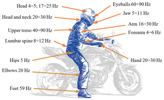
Figure 1.
Natural frequencies of selected organs and parts of the human body.
In order to reduce the effects of vibration on humans, it is critical to study the source of vibration, look for methods to reduce it, and evaluate the effects on the body. The permissible values and the exposure time are defined in the relevant standard [8], but it is more important to limit the possibility of vibration generation. Nevertheless, the evaluation of the effects of vibrations on humans is the subject of numerous studies and they also concern vibrations produced in the structure of a motorcycle. As an example, [9] measured the effects of vibration on a motorcyclist on seven different surfaces, using four motorcycles that differed in mass and geometric parameters. The placement of acceleration sensors is crucial. Unfortunately, it is not clear from the article how it was concluded that the vibrations are transmitted from the road and not the drivetrain. This is important because the only sensors that were mounted are on the sprung masses. Additionally, filtration and possible methods to isolate significant frequencies from the road surface were not discussed. However, it has been shown that the vibrations transmitted to the driver are of such magnitude that even with short exposure times, they can cause adverse effects on the human body.
In order to validate the analyses based on mathematical modeling and computer simulation, motorcycle motion and vibration tests are conducted using special test stands. Unfortunately, this type of research is relatively rarely described in scientific publications. Therefore, attention was drawn to [10], which describes experiments with a separate steering system of a motorcycle whose tire-wheel rotates on a sliding belt. On the other hand, in [11,12], bench tests are conducted using a partially immobilized motorcycle, whose front wheel cooperates with a rotating drum reflecting the road surface. The analyses presented in the following section are conducted based on the mathematical model described in [13], where its verification is described. Data for verification were recorded on a test rig, the operation of which can be seen at [14].
With the development of computer methods, mathematical models have become widely used. The motorcycle model described in [15] allowed the determination of the forms of vibrations that occur for the case of driving a motorcycle without using hands, named by the author as capsize, weave, and wobble. This already shows that with relatively simple models, it is possible to analyze the dynamics of a motorcycle [16]. Subsequently, research was extended to include mainframe susceptibility by both Sharp, as described in [16,17], and Kane [18]. It was thus shown that the stability of the motorcycle, and thus the weave vibration, is significantly affected by the stiffness of the mainframe, while it has no effect on the other two.
Unfortunately, very few models have been developed for frequency analysis of motorcycle steering vibrations. In particular, [19], which is a comprehensive book on the dynamics of a motorcycle, should be mentioned here. The influence of various structural parameters of a motorcycle on vibration damping at different speeds was analyzed in detail. It was concluded that the moment of inertia of the steering system could be important for the stability of a motorcycle, which is included in the expression derived from the single mass model. However, this model neglects many other steering parameters whose specific values may also contribute to vibration. Other works include [10,20,21,22], in which there is a determination of the natural frequency of the steering system. On the other hand, in [23], a single-mass model of the steering system dynamics with sharp nonlinearities is presented and applied to test numerical procedures, which is particularly important in solving differential equations by iterative methods.
Among the methods used to study the vibrations and their graphical presentation, we can mention [19,24,25,26], in which the graphs of the real part describing the vibrations as a function of driving speed are presented. The curves created in this way illustrate the dynamic properties of the motorcycle in a wide range of speeds and its tendency to unstable behavior well. The root locus plot was also used in [19,24], which allows one to observe changes in the damping of particular types of vibrations as a function of speed. On the other hand, in [27], the possibility of analyzing steering system vibrations by means of phase plane was presented, which can also be useful in vibration analysis.
During daily use, the mass of a motorcycle can change significantly. While the weight of the rider will be taken into account at the design stage, the presence of a passenger will change the weight distribution and front -heel loading; also, the fuel tank itself, when fully filled, will be an additional factor. Some improvement in motorcycle stability can be achieved by fitting a torsional vibration damper to the steering system. However, whether or not it is included in the steering system, every motorcycle should have a natural tendency to handle steadily. For this reason, it is important to look for parameters that have a key influence on steering dynamics and how they affect vibration frequency. Therefore, a method of analysis will be presented that will allow a complex description of the system to extract relevant information to assist in the design of a motorcycle.
2. Method and Tools Used
When modeling vibrations that are occurring in mechanical systems, certain simplifying assumptions are introduced—most often to replace the nonlinear model with a linear model. This approach to modeling results from the fact that the methods of analysis of linear systems are well developed and effective. In addition, nonlinear systems are often stable in some limited neighborhood of the equilibrium point only, while linear systems, if stable, are globally and, moreover, asymptotically stable [28]. The basic forms of description of the dynamics of linear dynamical systems (apart from differential equations) include the operator transmittance G(s) and the spectral transmittance G(jω). These such forms of description will be used later in this paper.
The physical model (Figure 2) directly corresponds to the motorcycle steering system mounted in a special drum test rig presented in [13]. It was also validated on the basis of the results of measurements made on this test stand.
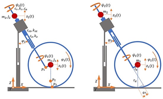
Figure 2.
Physical model of a motorcycle steering system.
This model considers the key features of a motorcycle steering system. It has five degrees of freedom, which are the rotational motion of the wheel about the wheel axis, the angular motion of the handlebars and wheel about the steering axis of the head tube, and the vertical motion of the wheel and body. Thus, the longitudinal operation of the suspension and its torsional compliance is taken into account. A simplified model of wheel-road interaction was adopted, neglecting the phenomenon of tire relaxation length, with a simplified description of the stabilizing moment based on [29,30,31]. Despite the simplifying assumptions made, it represents the steering dynamics well and is sufficient to demonstrate the analysis method presented in this paper. However, if necessary, any other model can be used, as the procedure will not change. This method is particularly useful at the initial stage of a motorcycle or other vehicle because it allows the selection of parameters of the real system and to study the vibrations that arise. However, in the final stage of design and modeling of individual parts, the finite element method can be used, as presented in [32], on the design of an elastic component for a motorcycle.
List of designations appearing in Figure 2 and in the equations described, along with values that are taken as references:
A system of nonlinear differential equations (initial model) was obtained using Lagrange’s equations of the second-order, and the most important formulas are presented below.
The potential and kinetic energy are written by Equations (2) and (3), and the energy dissipation is written by Equation (4).
Relevant to the driving wheel dynamics is the stabilizing torque, which is written as follows:
The parameter in Equation (5) is the actual overtaking distance and, taking into account the steering angle, its value can be calculated as follows:
The other components of generalized forces are:
and , which has a negative value, and the gravity forces , . The model also assumes the wheel slip is small, so the equation for the lateral force is expressed as follows:
and for the longitudinal force:
In the case under consideration, due to zero longitudinal slip, there will be no longitudinal force. For this reason, in the previously written equations also, some components related to the longitudinal force will be zero, but they are written for the sake of order since their absence could cause misunderstanding of the relations described.
Due to the adopted structure of the physical model, the obtained system of equations has a complex form. Therefore, symbolic transformation software (e.g., Maple, Octave) was used for their derivation as well as further transformations. This allowed the individual transmittances describing the ratio of the input signal to the output signal to be obtained and, most importantly, in the general form.
Ten different transmittances can be written for such a system, but four of them are important, namely: transmittance for vertical displacement of masses and at vertical excitation () and the transmittance for the angular displacements of masses and under torsional moment excitation ().
The process leading to the mentioned transmittances can be divided into different steps, which in order will be as follows:
- Development of the mathematical model;
- Linearization of the equations describing the system dynamics;
- Writing the equations in the operator form and determining the transmittance;
- Perform stability analysis of the system;
- Breaking down of transmittance into summation form;
- Frequency analysis of each of the members of transmittance.
On the other hand, analyses based on the transmittances obtained in this way were performed using the LabVIEW software and an application created for this purpose (Figure 3 and Figure 4).
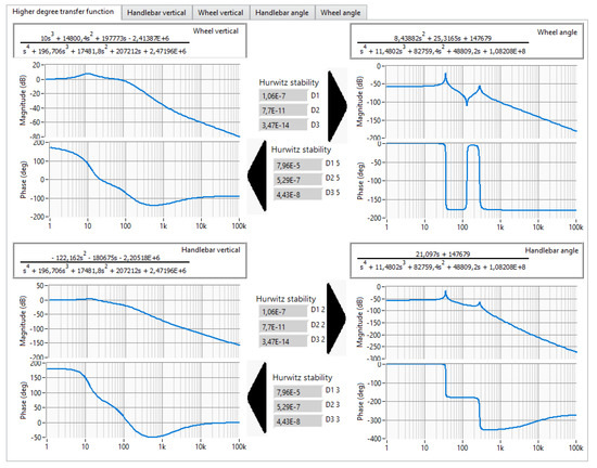
Figure 3.
View of the steering frequency analysis program window.
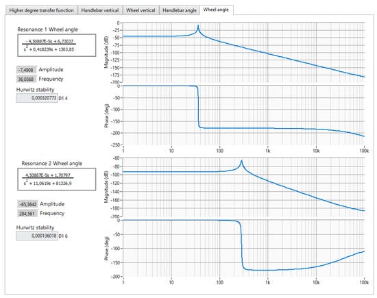
Figure 4.
View of the program window for frequency analysis of individual transmittances.
It is worth noting that the obtained strictly proper transmittances are of a higher order than is the case for the analyzed dual-mass models by other authors. However, it should be noted that, unlike the aforementioned models, the one presented here has a feature that has a key influence on its dynamics—the angle of inclination of the head of the frame.
As already mentioned, LabVIEW software was used to develop a suitable tool for breaking the higher-order transmittance down into two lower-order transmittances and analyzing the resulting Bode diagrams.
While breaking the transmittances down into simple fractions is relatively straightforward in this case, doing it automatically is not. The first problem one may encounter is finding zero places of the characteristic polynomial. In LabVIEW, the appropriate Partial Fraction Expansion (PFE) function is available, but in special cases, it does not return the correct result; and this case is one of them. The incorrect result, in some cases, results directly from the way the function is implemented. The PFE function uses the Heaviside function to calculate the residues and poles, which is not applicable when the roots of the polynomial in the denominator are either double or complex, so only single real roots will give the correct results. For this reason, it was not possible to use the appropriate VI from the palette.
This difficulty can be overcome by using a MathScript Node and a suitably written script. In this case, the script for finding the roots of the denominator polynomial is limited to two lines, where the first is an array of the coefficients of the polynomial and the second is the roots command. In this way, four composite roots are obtained. The final form, which is interesting from the perspective of further analysis, is obtained as follows. Having the denominator of the transmittance of the form:
and taking the expected form:
then, after writing the appropriate system of equations, one obtains the sought values of the coefficients a, b, c, d, e, f. Of course, a general form has been implemented in the program so that they are recalculated as the selected parameter changes (Figure 5).
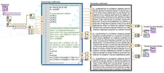
Figure 5.
View of a window with a code fragment of the steering frequency analysis program.
The second problem is the determination of the numerator factors. To obtain them in an analytical way, it is enough to take any real number as s and solve a system of equations. In this case, it cannot be done because in LabVIEW, the operator s does not appear directly in the equation, but only the coefficients of the polynomial. Therefore, it is necessary to use an additional tool for symbolic transformations and determine specific values of parameters by solving a typical equation in search of numerator factors.
The third problem that can be encountered is the implementation of the calculated numerator factors—solving a system of equations depending on the transmittance yields extremely large equations that take up dozens of A4 pages (between 40 and 80 pages). The problem that arises, in this case, is that too many lines of text are needed to be placed in the MathScript Node. This structure only holds about 20 pages of equations. If there are too many characters, they will not be processed by this structure, and an additional file corruption and LabVIEW critical error may occur. In some cases, using the Formula Node structure is sufficient. The final form of the code that allows the breaking down of the fourth-degree transmittance into two second-degree transmittances is shown in Figure 5.
The Formula Node structure takes three times as many characters, but even this may sometimes prove to be too few. However, this can be easily remedied by splitting the description of each coefficient into a single structure. This is also consistent with the idea of programming because the main code of the program should be divided into a subprogram.
Finally, the operation of the described program is presented in the diagram below (Figure 6). It is only one-quarter of the whole, but the remaining parts perform exactly the same calculations.
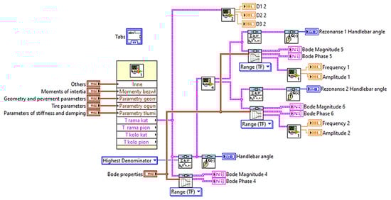
Figure 6.
View of a window with a code fragment of the steering frequency analysis program.
With the program thus developed, the Bode plots summarized below were obtained along with the significant values read from the plots.
When the values of the parameter are varied (Table 1), the tendency of the system to decrease in vibration frequency with increasing values of the moment of inertia can be observed, but not in a completely linear manner. This is true for both resonance frequencies. On the other hand, an increase in the parameter causes a significant decrease in the amplitude of vibrations of the wheel while increasing the amplitude of vibrations of the steering wheel. Noteworthy is the effect of the value of this parameter on the stability of the system in different frequency ranges. While for low-frequency resonance, the stability is slightly improved, for high-frequency resonance, a deterioration of stability by exactly the same value is observed. The observed changes in the oscillation period are directly related to the frequency, and it becomes longer as the moment of inertia increases while the relative damping decreases. Changing the value of the analyzed parameter also has a significant effect on the overall damping properties of the system, which decrease as increases.

Table 1.
The values of the parameters read from the graphs shown in Figure 7.
In the analyzed case, when the values of the parameter and are varied, the opposite situation to the one described earlier takes place, namely the change of the value of the wheel moment of inertia parameter affects the higher frequency vibrations to a greater extent. Changes in the value of the wheel moment of inertia parameter affect the resonance frequencies to a greater extent, and the nonlinearity of the changes is much more pronounced. The same relationship for stability is maintained for higher frequency resonance in this case; when increasing the value of moment of inertia increases, for lower frequency resonance, it decreases. The other values, such as vibration period and relative damping, have the same nature of changes, but their changes are more for the higher frequency resonance.
Previously, it could be observed (Figure 8, Table 2) that the moment of inertia of the wheel causes only slight changes in the low-frequency resonant vibration, while it affects the higher-frequency resonance. This case is similar (Figure 9, Table 3), while what is different is that the overall damping properties of the system no longer change so significantly.
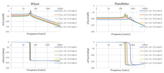
Figure 8.
Amplitude and phase characteristics of the steering angle position transmittance when the parameter values are changed Jx1 and Jz1.
Table 2.
The values of the parameters read from the graphs shown in Figure 8.
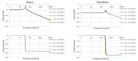
Figure 9.
Amplitude and phase characteristics of the transmittance of the steering angle position when the parameter value is changed Jy1.
Table 3.
The values of the parameters read from the graphs shown in Figure 9.
Looking at the graphs shown in Figure 10 and the data summarized in Table 4, which relate to the vertical displacement of the steering wheel, it can be concluded that low-frequency torsional vibration is only slightly transmitted to the vertical motion, while higher-frequency torsional vibration is transmitted to a greater extent. The system also shows much greater stability for vertical steering wheel vibration and damping than for torsional vibration. This is consistent with the actual behavior of the motorcycle, as no vertical self-excited vibration of the front of the motorcycle is observed, only torsional (wobble) vibration.
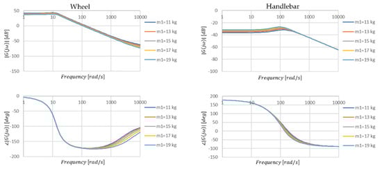
Figure 10.
Amplitude and phase characteristics of the transfer function of the handlebar angle position when the value of parameter m1 is changed.
Table 4.
The values of the parameters read from the graphs shown in Figure 10.
Compared to the previous graphs and values in the tables presented in Figure 11 and Table 5 show that the change of wheel mass causes only slight or even negligible changes in the analyzed values. On this basis, it can be concluded that the wheel mass does not significantly affect the torsional vibration despite some coupling of vertical and torsional motion through the advance section.
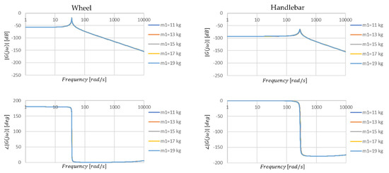
Figure 11.
Amplitude and phase characteristics of the transmittance of the steering angle position when the parameter value is changed m1.
Table 5.
The values of the parameters read from the graphs shown in Figure 11.
The graphs presented in Figure 12 and Figure 13 and the data in Table 6 and Table 7 allow us to conclude that the change in mass has little effect on vertical vibration and negligible effect on torsional vibration of the handlebars. This thus contradicts claims among motorcyclists that mass distribution affects wobble vibration. It is interesting to note, however, that despite changes in mass and changes in stability amplitude, vibration period, and damping, the frequency does not change for higher frequency vibrations.
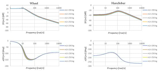
Figure 12.
Amplitude and phase characteristics of the transmittance of the vertical position of the steering wheel with a change in the value of the parameter m2.
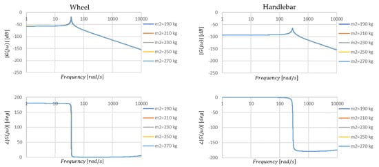
Figure 13.
Amplitude and phase characteristics of the transmittance of the steering angle position when changing the value of the parameter m2.
Table 6.
The values of the parameters read from the graphs shown in Figure 12.
Table 7.
The values of the parameters read from the graphs shown in Figure 13.
3. Discussion of Simulation Results
Complex models are not only difficult to interpret but also to identify a large number of parameters. The presented description of the program used shows not only the implementation of the method of analysis of system dynamics, but also the method of model reduction. This is a much simpler approach than the theory developed by Mandelstam to evaluate the coupling of partial sub-systems [33]. With Mandelstam’s theory, it is possible to break the full model down into a group of partial models. Another approach is parametric simplification, which addresses Hadamard’s postulate of continuity of solution changes with respect to model parameters [34]. However, both approaches are rarely used, because as a rule, partial models are extracted based on an a priori assumption about the weakness of the remaining interactions or the complete isolation of the system [33]. In the presented approach, the reduction can be obtained by breaking down the transmittance into a sum of factors. By omitting one of the lower order transmittances, a transmittance model of the system is obtained that is oriented towards the dynamics of the system in the range of selected vibration frequencies. However, this model is no longer in parametric form, which is indirectly related to the Abel–Ruffini theorem. In addition, depending on the values of the individual denominator factors, the breaking down into factors may or may not be performed, as the system will be unstable.
The system stability evaluation was performed using the Hurwitz method, but any other method can be used. This function has only been added to the program for your convenience and can be carried out separately using any other tool. The stability analysis indicates that the motorcycle’s steering is at the limit of stability. The small values of the third Hurwitz sub-designator confirm that the torsional vibration can be induced by the forces from the road irregularities. It can also be observed that in order to improve the stability of the system to vibrations of one frequency, we cause a deterioration of stability for the other frequency.
The computational results, shown in Figure 7, Figure 8, Figure 9, Figure 10, Figure 11, Figure 12 and Figure 13, although related to a selected portion of the simulation study, allow a number of interesting observations and conclusions to be drawn.
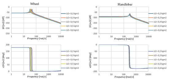
Figure 7.
Amplitude and phase characteristics of the steering angle position transmittance when the parameter value is changed Jz2.
After breaking the higher-order transmittance down into two lower-order transmittances, pairs of the same values characterizing the lower- and higher-order resonance for specific transmittance pairs are obtained. For example, the transmittance under impulsive excitation of the steering wheel and handlebar. It naturally follows that the resonant frequencies for two connected masses will also be two. Therefore, in the future, there is no need to analyze four Bode diagrams but only two.
The presented method by separating the two resonance frequencies greatly facilitates the inference of the behavior of the system depending on the parameters describing it. In particular with respect to damping properties and stability. The analysis, apart from confirming the obvious truths, i.e., increasing resonant frequencies with decreasing element mass, allowed us to notice some nonlinear changes in the system dynamics with linear changes in parameter values (Figure 8). While the mass of the road wheel may change slightly, e.g., depending on a more massive tire design, the use of different materials for the wheel structure (magnesium, carbon fiber) will cause changes in both the resonance frequencies of the wheel and steering wheel and their phase shifts (Figure 10). Such modification can be done by the user themself, as wheel rim replacements are now available.
The change in road wheel mass manifests itself only slightly through its effect on torsional vibration (Figure 11), although from the values (Table 5) the changes are noticeable. Despite the great importance of the wheel advance section for the handling stability of the motorcycle, the impacts due to vertical loads are transferred to a small extent to the torsional vibrations. Although using the total mass of the motorcycle as an example, an interesting relationship can be observed. As the mass increases, the damping of the system for vertical vibration also increases, but the stability and relative damping for torsional vibration decreases, which may indicate that increasing the mass of the motorcycle will increase the likelihood of torsional vibration occurring. Interestingly they will be at a higher frequency than for an unloaded motorcycle (Table 7). Therefore, if vibrations occur with a more heavily loaded wheel, the motorcycle will be more difficult for the rider to stabilize.
4. Summary and Conclusions
This paper presents a method of the breaking down of a system model into simpler components and the analysis of vibrations of particular frequencies, which can be applied in dynamics studies of not only motorcycles but also other systems. A mathematical model written in the form of operator transmittance was used, and on this basis, Bode diagrams were determined. The difficulties encountered in breaking down higher-order transmittances into simple fractions using the LabVIEW environment have been described in detail.
The method can be easily applied to more complex objects, which only requires the use of another mathematical model describing the investigated object. The results obtained in the numerical form also make it easier to grasp small substitutions, which may not be directly visible on the frequency characteristics but may be useful at the initial stage of machine design. With this method, it is possible to perform the model reduction in a formal way so that all relevant parameters are included in the final form of the model. It is relatively easy to obtain a simplified formula describing the dynamics of the system for a selected frequency and then develop a control system.
The driver, by deciding how to use the vehicle and making modifications to it, has an influence on the resonant frequencies of the steering system. However, typical operating factors do not cause significant changes, although they may contribute to the system’s sensitivity to vibration.
Funding
This research received no external funding.
Institutional Review Board Statement
Not applicable.
Informed Consent Statement
Not applicable.
Data Availability Statement
Data is contained within the article.
Conflicts of Interest
The authors declare no conflict of interest.
Abbreviations
| X, Y, Z | main axes of the coordinate system; |
| Mnk, Mb, Mor, Msk, W0 | a torque that adequately stimulates vibrations, driving from the drum and resistance to movement, steering, excitation from the road surface; |
| ψ1, ψ2 | the steering angle respectively of the wheel and handlebar; |
| φ1 | wheel rotation angle; |
| φ2 | steering head angle (24 deg); |
| z1, z2 | vertical displacement of the elements associated with the wheel and the frame, respectively; |
| J1, J2 | the equivalent moment of inertia of the components associated with the wheel (0.21 kgm2) and handlebar (0.4 kgm2), respectively; |
| m1, m2, m | reduced weight of the components associated with the wheel (15 kg) and frame (230 kg), and sum of masses m1 i m2, respectively; |
| cr, ca, csz, cz, Co | damping coefficient of the driver’s hands (0.2 Nms/rad), torsional vibration damper (0 Nms/rad), torsional damping of suspensions (3 Nms/rad), longitudinal damping of suspension (2.6 kNs/m), tire damping coefficient (150 Ns/m), respectively; |
| kr, ksz, kz | stiffness coefficient of the driver’s hands (1 kN/rad), torsional stiffness (7 kNm/rad), longitudinal stiffness (14 kN/m), respectively; |
| Kz, Kα, Kx | radial tire (190 kN/m), cornering stiffness coefficient (10 kN/rad), longitudinal stiffness coefficient (180 kN/m), respectively; |
| p1, p2, p3 | the point of suspension end, wheel rim, and wheel/road contact, respectively; |
| rd | dynamic wheel radius (0.3 m); |
| l, l1, lk | wheelbase (1.35 m), distance between the center of mass and the front wheel’s axis of rotation (0.6 m), offsetting the wheel axis from the control axis of the frame head (0.03 m); |
| wpo | tire profile height (0.08 m); |
| a1 | actual overtaking distance (0.1 m); |
| ω | angular velocity; |
| χ | wheel camber angle; |
| Fx, Fy, Fz | longitudinal, lateral, and vertical reaction forces, respectively; |
| ex | displacement of normal force; |
| Sx | longitudinal slip. |
References
- Piantini, S.; Pierini, M.; Delogu, M.; Baldanzini, M.; Franci, A.; Mangini, M.; Peris, A. Injury Analysis of Powered Two-Wheeler versus Other Vehicle Urban Accidents. In Proceedings of the 2016 IRCOBI Conference; IRCOBI: Malaga, Spain, 2016. [Google Scholar] [CrossRef]
- Prochowski, L.; Pusty, T. Charakterystyka Obrotu i Unoszenia Motocykla po Uderzeniu w Bok Samochodu; The Archives of Automotive Engineering (Archiwum Motoryzacji): Warszawa, Poland, 2012. [Google Scholar]
- Wypadki drogowe w Polsce w 2019 roku; Technical Report; Biuro Ruchu Drogowego Zespół Profilaktyki i Analiz: Warszawa, Poland, 2020.
- Stan bezpieczeństwa ruchu drogowego oraz działania realizowane w tym zakresie w 2019r. Available online: https://www.krbrd.gov.pl/baza-wiedzy/raporty-o-stanie-brd/ (accessed on 18 August 2021).
- Dukalski, P.; Będkowski, B.; Parczewski, K.; Wnęk, H.; Urbaś, A.; Augustynek, K. Dynamics of the vehicle rear suspension system with electric motors mounted in wheels. Eksploat. I Niezawodn. Maint. Reliab. 2019, 21, 125–136. [Google Scholar] [CrossRef]
- Nader, M.; Korzeb, J. Przegląd Biomechanicznych Modeli do Oceny Oddziaływania Drgań na Organizm Ludzki, Materiały III Krajowego Sympozjum, Komputerowe Systemy Wspomagania Prac Inżynierskich w Przemyśle i Transporcie; Politechnika Radomska: Zakopane, Poland, 1999. [Google Scholar]
- Praca Zbiorowa, Tłumienie Drgań. 1997. Available online: https://tezeusz.pl/tlumienie-drgan-zbigniew-osinski?sortowanie=cena_malejaco (accessed on 18 August 2021).
- International Organization for Standardization. ISO-2631—Mechanical vibration and shock. In Evaluation of Human Exposure to Whole-Body Vibration; ISO: New Dheli, India, 1997. [Google Scholar]
- Shivakumara, B.S.; Sridhar, V. Study of Vibration and Its Effect on Health of the Motorcycle Rider; Online Journal of Health and Allied Sciences Peer Reviewed, Open Access; Free Online Journal Published Quarterly: Mangalore, South India, 2012; Volume 9, ISSN 0972-5997. [Google Scholar]
- Di Massa, G.; Pagano, S.; Strano, S.; Terzo, M. A Mono-axial Wheel Force Transducer for the Study of the Shimmy Phenomenon. In Proceedings of the World Congress on Engineering, London, UK, 3–5 July 2013. [Google Scholar]
- Grzegożek, W.; Weigel-Millert, K. Analiza możliwości wykorzystania badań stanowiskowych do oceny stabilności pojazdu jednośladowego. Arch. Automot. Eng. Arch. Motoryz. 2015, 67, 165–173. [Google Scholar]
- Ślusarczyk, P. Analiza Modelowa Stateczności Pojazdu Jednośladowego, Czasopismo Techniczne; Wyd, P.K., Ed.; Zeszyt 7-M: Kraków, Poland, 2004; pp. 165–173. [Google Scholar]
- Dębowski, A. Analiza Możliwości Ograniczenia Drgań Skrętnych w Układzie Kierowniczym Motocykla, Rozprawa Doktorska; Military University of Technology: Warszawa, Poland, 2019. [Google Scholar]
- Available online: http://andrzejdebowski.wat.edu.pl/galeria.html (accessed on 14 April 2021).
- Sharp, R.S. The stability and control of motorcycles. J. Mech. Eng. Sci. 1971, 13, 313–329. [Google Scholar] [CrossRef] [Green Version]
- Sharp, R.S. The Influence of Frame Flexibility on the Lateral Stability of Motorcycles. J. Mech. Eng. Sci. 1974, 16, 117–120. [Google Scholar] [CrossRef]
- Sharp, R.S.; Alstead, C.J. The influence of structural flexibilities on the straight-running stability of motorcycles. Veh. Syst. Dyn. 1980, 9, 327–357. [Google Scholar] [CrossRef]
- Kane, T.R. The Effect of Frame Flexibility on High Speed Weave of Motorcycles; SAE Technical Paper 780306; SAE International: Warrendale, PA, USA, 1978. [Google Scholar]
- Cossalter, V. Motorcycle Dynamics; LULU: Morrisville, NC, USA, 2006. [Google Scholar]
- Cossalter, V.; Lot, R.; Massaro, M. An Advanced Multibody Code for Handling and Stability Analysis of Motorcycles; Springer Meccanica: Berlin/Heidelberg, Germany, 2011; Volume 46, pp. 943–958. [Google Scholar] [CrossRef]
- De Falco, D.; Di Massa, G.; Pagano, S.; Strano, S. Wheel Force Transducer for Shimmy Investigation. In Proceedings of the World Congress on Engineering, London, UK, 1–3 July 2015. [Google Scholar]
- Sharp, R.S.; Limbeer, D.J.N. On steering wobble oscillations of motorcycles. J. Mech. Eng. Sci. 2004, 14, 1449–1456. [Google Scholar] [CrossRef] [Green Version]
- Żardecki, D.; Dębowski, A. Badania procedur obliczeniowych pod kątem zastosowań w symulacji drgań skrętnych w układzie kierowniczym motocykla z uwzględnieniem luzu i tarcia. Arch. Automot. Eng. 2014, 64, 79–95. [Google Scholar]
- Pacejka, H. Tyre and Vehicle Dynamics; Elsevier: Waltham, MA, USA, 2012. [Google Scholar]
- Sharp, R.S. A Review of Motorcycle Steering Behaviour on Straight Line Stability Characteristics; SAE Paper n 780303; SAE International: Warrendale, PA, USA, 1978. [Google Scholar] [CrossRef]
- Sharp, R.S.; Watanabe, Y. Chatter vibrations of high-performance motorcycles, Vehicle System Dynamics. Int. J. Veh. Mech. Mobil. 2013, 51, 393–404. [Google Scholar]
- Żardecki, D.; Dębowski, A. Metoda Analizy Drgań Skrętnych w Układzie Kierowniczym Motocykla na Płaszczyźnie Fazowej. Arch. Automot. Eng. 2017, 72, 137–154. [Google Scholar]
- Praca Zbiorowa: Zarys Dynamiki i Automatyki Układów. 1991. Available online: https://bcpw.bg.pw.edu.pl/Content/767/PDF/01zdau_poczatek.pdf (accessed on 18 August 2021).
- Adamiec-Wójcik, I.; Maczyński, A.; Wojciech, S. Zastosowanie Metody Przekształceń Jednorodnych w Modelowaniu Dynamiki Urządzeń Offshore; Wydawnictwo Komunikacji i Łączności: Warszawa, Poland, 2008. [Google Scholar]
- Bhargava, A. Algorytmy. In Ilustrowany przewodnik; Wydawnictwo Helion: Gliwice, Poland, 2017. [Google Scholar]
- Chang, Y.P.; El-Gindy, M.; Streit, A. Literature survey of transient dynamic response tyre models. Int. J. Veh. Des. 2004, 34, 354–386. [Google Scholar] [CrossRef]
- Mann, V.; Dechwayukul, C.; Thongruang, W.; Srewaradachpisal, S.; Kaewpradit, P.; Kaew Apichai, W.; Bui, H.-T. Design and Fabrication a Lightweight Spring Made of Natural Rubber for a Motorcycle’s Shock Absorber. Int. J. Automot. Mech. Eng. 2020, 17, 7758–7770. [Google Scholar] [CrossRef] [Green Version]
- Stańczyk, T.L. Metoda Modeli Częściowych Jako Podstawa Tworzenia Komputerowych Systemów Analizy Dynamiki Złożonych Układów Mechanicznych; Rozprawa Habilitacyjna, Politechnika Świętokrzyska: Kielce, Poland, 1994. [Google Scholar]
- Żardecki, D. Modelowanie i Badania Symulacyjne Dynamiki Ruchu Samochodu z Uwzględnieniem Luzu i Tarcia w Układzie Kierowniczym z Zastosowaniem Odwzorowań luz(…) i tar(…). In Proceedings of the Konferencja Między Teorią a Zastosowaniami: Matematyka w Działaniu, Poznań, Poland, 17–20 September 2014. [Google Scholar]
Publisher’s Note: MDPI stays neutral with regard to jurisdictional claims in published maps and institutional affiliations. |
© 2021 by the author. Licensee MDPI, Basel, Switzerland. This article is an open access article distributed under the terms and conditions of the Creative Commons Attribution (CC BY) license (https://creativecommons.org/licenses/by/4.0/).