Article

Heterogeneous Inertia Estimation for Power Systems with High Penetration of Converter-Interfaced Generation

Institute for Automation of Complex Power Systems, E.ON Energy Research Center, RWTH Aachen University, 52062 Aachen, Germany
*
Author to whom correspondence should be addressed.
Energies 2021, 14(16), 5047; https://doi.org/10.3390/en14165047
Submission received: 14 July 2021 / Revised: 11 August 2021 / Accepted: 13 August 2021 / Published: 17 August 2021
(This article belongs to the Special Issue Frequency Stability and Control in Future Power Systems)

Abstract

:
The increasing and fast deployment of distributed generation is posing challenges to the operation and control of power systems due to the resulting reduction in the overall system rotational inertia and damping. Therefore, it becomes quite crucial for the transmission system operator to monitor the varying system inertia and damping in order to take proper actions to maintain the system stability. This paper presents an inertia estimation algorithm for low-inertia systems to estimate the inertia (both mechanical and virtual) and damping of systems with mixed generation resources and/or the resource itself. Moreover, the effect of high penetration of distributed energy resources and the resulting heterogeneous distribution of inertia on the overall system inertia estimation is investigated. A comprehensive set of case studies and scenarios of the IEEE 39-bus system provides results to demonstrate the performance of the proposed estimator.

1. Introduction

Traditionally, the operation of power systems is based on rotating Synchronous Generators (SGs). Due to the electromechanical coupling between the SG rotational speed and the electrical grid frequency, the inertia of the SGs rotating masses plays a crucial role in maintaining the system stability. SGs inherently release (absorb) kinetic energy following any active power imbalance that would result in a frequency drop (increase).
Increasing the penetration of Distributed Energy Resources (DERs), which are connected to the grid through power converters, and their replacement of SGs, has led to low-inertia power systems and areas. Frequency variations are faster and larger in low-inertia systems; consequently, low-inertia power systems have lower stability margins, and their control is more challenging. Furthermore, not only is the amount of inertia reduced, but inertia has also become uncertain and time-variable. The merging issue of low-inertia power systems and their implication for power system stability and operation has been addressed in [1].
The mitigation solution for large frequency excursions and high rates of change of frequency (RoCoF) in low-inertia systems is to enable converter-interfaced distributed generation, through supplementary control and energy storage, to provide frequency support within 1 s after a disturbance as an ancillary service. This frequency support can be achieved through two approaches, mainly: fast frequency regulation (FFR), in which the DER adjusts its output active power, according to the frequency deviation and the virtual inertia provision, in which the DER mimics the SG inertia response and adjusts its output active power according to the RoCoF. FFR is already being adopted as an ancillary service in low-inertia systems; such as Ireland, UK, New Zealand and the Nordic power system [2].
However, some open questions remain; what is the minimum amount of rotational inertia that needs to be present in the system ahead of real-time operation? What is the adequate amount of FFR and/or virtual inertia reserve that needs to be procured? The answers can be obtained by determining the amount of inertia in the system at any given time. Moreover, such knowledge also enables system operators to take proactive control and protection actions in real time, thus enhancing the system stability and resulting in economic benefits.
In the last decade, a large amount of literature on inertia estimation methods has emerged, and different Transmission System Operators (TSOs), such as the Nordic System, National Grid ESO and ERCOT, have been using such methods. A very simple approach has been used to estimate the inertia of the Nordic system based on the status of the circuit breaker of conventional SGs [3]. However, such an approach requires monitoring of all circuit breaker positions and an accurate knowledge of the different SGs inertia constants and capacity. Given this limitation, methods that directly work with the time series of frequency and active power data have been the focus of researchers. Such methods estimate the inertia following a disturbance based on (1) inter-area oscillations and modal analysis or (2) simplified swing equation models.
The approaches based on inter-area oscillations, such as the method presented in [4], are complex, require different steps in order to estimate the inertia and are suitable for conventional power systems. A coherency analysis needs to be carried out in order to group the system into two areas swinging each other and then accurate modal analysis needs to be conducted.
The simplified swing equation model estimates the inertia from the RoCoF calculation directly post-disturbance as in [5,6]. In [5], averaging window filters are used on the active power and RoCoF measurements, then the inertia constant of individual generators is calculated and the sum is taken to find the total inertia. This approach depends on the accurate detection of the time of the disturbance. In [6], the authors adopt a similar approach, but to estimate the total system inertia, and they use the detrended fluctuation analysis to detect the time of the disturbance. However, these direct calculation approaches, based on the simplified swing equation, neglect the effect of load frequency and voltage dependency and the SGs control loops that affect the system frequency dynamics. Hence, they can result in estimation errors of up to 40%, as shown in [7].
The effect of the load frequency dependency and the primary frequency control of generator’s governors was taken into account in the offline estimation approach presented in [7]. In [8], the power demand changes of the load due to their voltage dependency has been taken into account. However, this method only works well in the unrealistic case in which the loads of the system coincide with the constant current load model of the estimation method.
So far, the methods presented are offline and use a linearized and simplified swing equation, typically ignoring factors that affect frequency damping and/or load voltage dependency. Additionally, they require a pre-knowledge of the size of the disturbance. A statistical model is proposed in [9] to estimate the system inertia variations from the small frequency variations during normal operation. However, this method requires a large amount of historical data and SGs dispatch information to calculate the base system inertia and then estimate the small variations in inertia. Similarly, in [10], the authors propose a method to estimate the so-called effective inertia, including the effect of load contributions and the primary frequency control action of the system online and from small frequency variations. Using a grey-box identification method, based on linear regression of large amounts of measurements, the system ARMAX model is obtained and then system identification is applied. Nevertheless, this approach does not have high accuracy. In [11], an estimation method has been proposed to estimate the effective inertia, which includes the equivalent inertia of converter-interfaced generation coupled to FFR, of power systems with high penetration levels of wind turbines. This approach requires the accurate detection of the disturbance and the angular swing first peak. Moreover, the limitation of effective inertia estimation is that it is only possible during a very short time window where a linear relationship is assumed, as highlighted in [12]. In [13], an inertia and damping estimation approach is proposed to track these parameters for both SGs and converter-interfaced generation. However, this approach is limited to estimating the equivalent inertia of a single resource and not the inertia of the whole system. Furthermore, the approach in [13] fails in estimating the damping of SGs.
Dynamic Regression and Extension Method (DREM) is applied in [14] to estimate the overall inertia of the system and the system set-point mechanical power online. The proposed method works in close to real-time and has been proven to work online in real-time following generator rescheduling events which take place on an hourly basis. The approach has high accuracy due to the fact that it takes into account the SGs Primary Frequency Control (PFC) action and does not attempt to linearize the system model. Consequently, this approach is deemed as the best presented solution. However, the proposed estimator requires knowledge of the PFC parameters and does not estimate the damping coefficient. Consequently, it cannot be used to estimate the amount of damping and virtual inertia provided by converter-interfaced generation.
Although a large literature on inertia estimation methods is available, they have not studied the effect of heterogeneous inertia on the inertia estimation so far. In the aforementioned approaches, the effect of the inertia heterogeneity, in terms of spatial distribution and inertia source, has not been investigated. Moreover, the damping factor and the fast primary control, which are critical for system stability and frequency control reserve sizing in the presence of DERs, are either neglected or included in the so called effective/equivalent inertia, without separation between damping and inertia that is relevant for proper sizing of frequency reserves and accurate stability studies.
To address the above concerns, this paper presents a novel method for the online estimation of power system inertia and damping, including both mechanical and virtual inertia. This method captures the effect of load damping and fast frequency control contributions and provides improved accuracy with respect to the literature and does not require the knowledge of the PFC parameters. Besides, this method can be used to identify the control parameters of converter-interfaced generation, which is typically considered as a black box by system operators. Finally, the effect of inertia heterogeneity and the timescale difference of the PFC and FFR on the inertia and damping estimation performance in power systems with mixed generation is analysed. To the best of the authors’ knowledge, such a comprehensive study has not been addressed in the literature so far.
We start by extending the DREM approach [14] to estimate the damping coefficient in addition to the inertia constant resulting from SGs and virtual inertia sources by applying the DREM method to an aggregated frequency dynamics model of a low-inertia system containing converter-interfaced generation participating in frequency control through droop control and VSM control strategies. Subsequently, verification of performance of the proposed estimation approach in terms of the estimation accuracy is carried out via Matlab/Simulink simulation studies on the modified IEEE 39-bus system. Furthermore, it is demonstrated that the estimation method can work in normal operation conditions with small load variations. Finally, the effect of heterogeneous inertia on the overall system estimation is investigated and we show that the inertia and damping estimation need to be carried out at a zone or area level to suit the regional nature of low-inertia parts of the grid.
The remainder of this paper is organized as follows: Section 2 introduces a model of frequency dynamics of power systems with mixed generation. Section 3 presents the parameterization and regression model and reviews the DREM approach. In Section 4, two case studies are considered to evaluate the performance of the proposed method and investigate the effect of mixed generation on the system inertia and damping estimation. Finally, Section 5 summarizes the obtained results and draws the conclusions of this paper.

2. System Frequency Dynamics

This section introduces the frequency dynamics model for synchronous power systems, which constitutes the reference model for the parametric estimation method used for the inertia estimation. A low-inertia power system, comprised of conventional SGs ( i N S G ) and aggregated converter-interfaced DERs is considered.
The frequency dynamics in such a system are governed by the electromechanical dynamics of synchronous generators and the control of power converters. Moreover, the frequency dependency of loads affects the frequency dynamics.
In the following subsections, the dynamics of synchronous generators and power converters, in addition to load frequency dependency, are recalled and their relation to the power system frequency is established with regard to our work.

2.1. Synchronous Generators Dynamics

The electromechanical dynamics of a SG can be expressed in terms of the classical nonlinear Swing Equation (SE), which relates the rotating masses angular speed ω to the active power imbalance, as:
2 H i S B , i ω 0 ω ˙ i ( t ) = ω 0 ω i ( t )   ( P m , i ( t ) P e , i ( t ) )
where i denotes generator ( i N S G ). H is the inertia constant and S B is the rated power of the SG, P m and P e are the reference mechanical power and output electrical power, respectively. When the system is in equilibrium state, i.e., the generation meets the load demand P m = P e , the angular speed ω = 2πf and the system frequency f are equal to their nominal values   ω 0 and f 0 , respectively.
As indicated in (1), following a disturbance, two quantities mainly determine the principal open-loop (i.e., without additional control loops) dynamic behavior of SGs: the amount of active power imbalance Δ P = P m P e resulting from the disturbance and the kinetic energy stored in the rotating masses of the generator, which is related to the inertia constant. The larger the inertia, the slower the Rate of Change of Frequency (RoCoF), i.e., ω ˙ .
In power systems, different frequency control structures (the primary, secondary and tertiary frequency control) with different timeframes are needed to maintain the system frequency stability in the presence of active power imbalances. However, we are concerned with the Primary Frequency Control (PFC) action, which has a control action timeframe of 1−30 s and so it affects the frequency dynamics of the system shortly after a disturbance and as a result influences the inertia estimation. Moreover, the PFC control affects the amount of the system damping.
The PFC is done locally, based on the set-points for frequency and power. Any deviation from the set-points results in a control signal that will influence the prime mover of the SG in order to increase or decrease the active power generation to meet the system needs, so that the deviation in the frequency of the system Δ ω ( t ) = ( ω ( t ) ω 0 ) , is contained.
The proportional feedback control adjusts the power generation set-point of the generator according to the frequency deviation, as follows:
P m ( t ) = P * + u ( t ) = P * K S G Δ ω ( t )
Note that the SG turbine dynamics play an important role in the PFC action by introducing time delays in changing the SG output power. The turbine dynamics of conventional thermal SGs can be described using the following model:
P F C ( t ) = 1 + s T z 1 + s T p K S G Δ ω ( t )
Consequently, including a PFC action in SG i , the swing equation takes the following form:
2 H i S B , i ω 0 ω ˙ i ( t ) = ω 0 ω i ( t )   ( P i * + P F C i ( t ) P e , i ( t ) )

2.2. Frequency Dynamics of Grid-Forming Converter-Interfaced Generation

Most power electronic converters connected to the grid today are grid-following converters, in other words they require a connection to a strong grid to be able to synchronize and they do not adjust their output power according to the system needs. Such converters can be modelled as loads with negative demand.
In this section, we are mainly interested in converter-interfaced generation, which is controlled according to the so-called grid-forming control strategies, which have strong influence on the frequency dynamics.
The literature on grid-forming converters can be mainly categorized into droop control and Virtual Synchronous Machine (VSM). The droop control emulates the SG primary frequency control action; however, converters provide FFR due to the fact they do not have rotating bulky parts, hence their time constant T c   is small and their response can be more than ten times faster than SGs.
F F R ( t ) = 1 1 + s T c K d r o o p Δ ω ( t )
Given the common assumption that the droop control is based on proportional control and does not provide virtual inertia, i.e., H d r o o p = 0 , the frequency dynamics model are as follows:
2 H d r o o p S d r o o p ω 0 ω ˙ d r o o p ( t ) = P * + F F R ( t ) P e ( t ) = 0
The VSM, on the other hand, emulates the behavior of SGs based on the swing equation; thus, the control includes the derivative term:
2 H V S M S V S M ω 0 ω ˙ V S M ( t ) = P * 1 1 + s T c K V S M Δ ω ( t ) P e ( t )
where the emulated inertia constant is defined as H V S M   and the emulated damping is K V S M . It is worth mentioning that the emulated damping in the VSM implementation in (7) maps directly to the FFR of the droop controller. The internal speed or angular frequency and the rated power of the VSM are ω V S M   and S V S M , respectively. Given that T c is quite small, the time delay in the VSM virtual inertia provision is ignored in the following sections.
As shown, the VSM dynamic behavior is quite similar to SGs. However, it is worth noting that the damping and inertia coefficients of VSMs are not related to physical properties but rather to control parameters and available amount of energy storage.
For simplicity, in what follows the term machine for both SGs and converters emulating SGs is used and the term inertia denotes both mechanical and virtual inertia.

2.3. Aggregated Frequency Dynamics

For a system containing a set of N = N S G   N V S M   N d machines, comprised of N S G synchronous generators, N V S M VSM controller interfaced generation and N d droop controller interfaced generation, the system frequency dynamics can be represented with one single aggregated swing equation, through assuming strong coupling between local frequencies and summing the frequency dynamics of individual machines ( j N ), which results in the center of inertia frequency dynamics [15] as follows:
2 H s y s S B , s y s ω 0 ω ˙ s y s ( t ) = ω 0 ω s y s ( t ) Δ P ( t )
where S B , s y s is the rated power of the system, H s y s is the total inertia constant of the system constituting mechanical and virtual inertia, calculated as follows:
H s y s = j N H j S B , j S B , s y s
The center of inertia frequency ω C O I depends on the inertia constants of the individual machines and may be calculated as a weighted average, as follows:
ω C O I ( t ) = j N H j S B , j ω j ( t ) j N H j S B , j
Assuming that the inertia constants are unknown and our aim is to estimate them, similar to the approach proposed in [14], the system average frequency, ω a v g = j N ω j N , is used instead. The power imbalance Δ P ( t ) is given as follows, including the mismatch between the total scheduled generation P s y s * and the total load demand P e , s y s ( t ) in addition to the total frequency control actions in SGs and FFR of both VSM-interfaced generation and droop-interfaced generation, the P F C S G ( t ) ,   F F R V S M ( t )   a n d   F F R d r o o p ( t ) , respectively.
Δ P ( t ) = P s y s * P e , s y s ( t ) + P F C S G ( t ) + F F R V S M ( t ) + F F R d r o o p ( t )
Part of the loads in the power system are dependent on the frequency of the system. In fact, the loads frequency dependency is quite important for power systems stability as it has a stabilizing damping effect on the frequency. Thus, this dependency is typically modelled by the damping coefficient   D L o a d . The total load demand decreases according to the drop in the system frequency, as follows:
Δ P L ( t ) = D L o a d Δ ω a v g ( t )
Including the load frequency dependency into the overall system dynamics (8) and using per-unit values of active power and frequency results in the following frequency dynamics model:
ω ˙ a v g ( t ) = 1 2 H s y s ω a v g ( t ) ( P s y s * P e , s y s ( t ) Δ ω a v g ( t ) × ( K S G × 1 + s T z 1 + s T p + K V S M × 1 1 + s T c + K d r o o p × 1 1 + s T c + D L o a d ) )
with the respective parameters defined as follows:
K S G = i N g K S G , i × S B , i S B , s y s K V S M = k N V S M K V S M , k × S B , k S B , s y s K d r o o p = l N d K d r o o p , l × S B , l S B , s y s
which indicates that the VSM emulated damping, the droop control gains and the load frequency dependency contribute to the overall damping of the system. At steady state, the total damping of the system:
D s y s = K S G + K V S M + K d r o o p + D L o a d

3. Parameterization and Regression

Our estimation approach is based on the DREM [14], a novel approach for parameters estimation using scalar regression models. In [14], the proposed model parameterization assumes prior knowledge of the PFC control action parameters and neglects the load frequency dependency in order to estimate the system inertia and active power set-point. In contrast to the problem formulation and parameterization used in [14], two alternative problem parameterizations are proposed by considering the problem of estimating the system inertia H s y s and damping D s y s . The proposed approach results in an improved estimation accuracy and enables the identification of the frequency control parameters of converters interfacing DERs to the grid and providing FFR or/and virtual inertia.
Considering the system (13), the active power and frequency measurements of generating units are assumed to be available for the TSO through the Wide-Area Measurement Systems (WAMS) and that the TSO has access to the active power set-points and the parameters of synchronous generators PFCs as part of the system operation planning.
With that information available, ω a v g ,   P e , s y s ( t ) ,   P s y s *   a n d   P F C S G ( t ) can be obtained and the system inertia and the damping provided by the rest of the system can be estimated. If the converters FFR parameters are also available, the   F F R V S M ( t )   and   F F R d r o o p ( t ) can be calculated and D L o a d can be estimated. However, the assumption on the knowledge of the PFC and FFR parameters is not always needed, as demonstrated in Section 4.2.
Starting with the general parameterization of system (13), by defining the input of our system as the active power imbalance in per unit and the output as the average system frequency in per unit as follows:
x ( t ) = P s y s * P e , s y s ( t )                                 y ( t ) = ω a v g ( t )
with the constant:
b = 1 2
and the system inertia H s y s and damping D s y s as parameters to estimate:
η 1 = 1 H s y s                         η 2 = D s y s H s y s
yielding the following system parameterization:
y ˙ = b η 1 ( x y ) b η 2 ( Δ y y )
In the case that partial information on the system damping is available, such that PFC and/or FFR parameters are known, these control actions are to be taken in the active power imbalance as an input to the system:
x ( t ) = P s y s * P e , s y s ( t ) + P F C S G ( t ) + F F R V S M ( t ) + F F R d r o o p ( t )
which yields an alternative parameterization:
η 2 = D L o a d H s y s
The effect of the two possible parameterizations is studied in Section 4.2.
Using the system dynamics (16), the regression [14] is constructed by applying the filter α s + α with α > 0 to (16):
α s s + α y = η 1 α s + α b ( x y ) η 2 α s + α b ( Δ y y ) + ϵ
where ϵ is an exponentially decaying term, resulting from the filter’s initial conditions. The term ϵ is neglected to simplify representation.
Consequently, the regression model can be written as follows:
z = η 1 ϕ 1 + η 2 ϕ 2 + ϵ = ϕ T η
where z = α s s + α y , ϕ 1 = α s + α b ( x y ) and ϕ 2 = α s + α b ( Δ y y ) .
Subsequently, a delay operator is introduced to extend the dimension of the regressor (18) from 1 to 2, in order to be able to estimate the two unknown parameters, yielding the following delayed regressor:
z d e l a y = z ( t d ) = ϕ T ( t d ) η = ϕ d e l a y T η
Augmenting the original regressor (18) with the delayed regressor (19) yields the following extended regression:
[ z z d e l a y ] = [ ϕ T ϕ d e l a y T ] η = Φ η
Multiplying (20) by the adjunct matrix of Φ , the decoupled regression is obtained:
Z = [ Z 1 Z 2 ] = a d j ( Φ ) Φ η = d e t ( Φ ) η
where Z = a d j ( Φ ) * [ z z d e l a y ] . Finally, η can be estimated using the gradient descent approach:
η ^ ˙ 1 = γ 1 d e t ( Φ ) ( Z 1 d e t ( Φ ) η ^ 1 )             η ^ ˙ 2 = γ 2 d e t ( Φ ) ( Z 2 d e t ( Φ ) η ^ 2 )      
where γ 1 and γ 2 are the learning rates of the gradient descent.

4. Simulation-Based Analysis

The proposed estimation method and the effect of heterogeneous inertia is investigated and evaluated on a modified version of the IEEE 39-bus New England benchmark test system, which is widely used for stability studies and performance evaluation of monitoring and control concepts. The detailed dynamic model of the benchmark system is simulated using detailed EMT models in Matlab/Simulink.
The single-line diagram of the New England 39-bus, 10-machine test system is depicted in Figure 1. The network model also includes 19 loads and full-order model of synchronous generators. Additionally, SGs are equipped with Power System Stabilizers, Automatic Voltage Regulators and PFCs. The dynamic data of the New England 39-bus can be found in [16].
In the modified version of the IEEE 39-bus, a nominal system frequency of 50 Hz is considered and the inertia of the rotating masses is set as summarized in Table 1. The SGs implement PFC control with a droop coefficient of 0.05 and a time constant of 5 s.
Furthermore, to take into account the effects of DERs providing frequency support, the benchmark system is modified by replacing four SGs with grid-forming converters of the same capacity and operating set-points. It is worth mentioning that each grid-forming converter unit represents an aggregation of DERs participating in frequency control and the virtual inertia and damping parameters are lumped parameterization of the aggregate behaviour. SG8, SG9 and SG10 are replaced with droop converters and SG5 is replaced by a VSM converter with the same inertia constant to reflect emerging future scenarios, where some regions of the power system depends heavily on DERs providing frequency support and other regions with conventional generation. Moreover, more droop than VSM control is considered, because of current trends. Modelling preliminaries of grid-forming converters have been previously introduced in Section 2.3. The converters droop is set to 5% and assume that the converter is interfacing a battery energy storage source with a DC source time constant of 50 ms.
The sampling time of the simulation measurements is chosen, such that the dynamics of the different machines are captured.
In the following subsections, the accuracy and applicability of the proposed estimation approach is analysed by means of Case Study I on the IEEE 39-bus system, depicted in Figure 1a, consisting of synchronous generation only. Subsequently, in Case Study II the applicability of the estimation method for mixed generation is validated on the modified IEEE 39-bus system shown in Figure 1b, and the effect of heterogeneous inertia and the different timescales of frequency control on the inertia and damping estimation is investigated.

4.1. Case Study I: Estimation Performance and Validation

As proof of concept, in Case Study I, the inertia estimation performance is investigated in the base case system, i.e., the 39-bus system with SGs and total system inertia, calculated using Equation (9), H s y s = 3.32 s. In our simulations, the effect of realistic load profiles, in terms of stochastic load variations, on the inertia estimation is considered, by modelling the system loads as time series of constant power loads with power profiles adopted from real-world measurements obtained from the 125 kV sub-transmission system of the city of Lausanne in Switzerland [17].
In this respect, at t = 80 s, a load step of 0.035 p.u is applied to the system with different load profiles, causing a power imbalance and consequently resulting in a change in the average system frequency as shown in Figure 2.
In the base scenario, i.e., with constant load profiles, the estimation of the system inertia converges within 5 s with a steady state estimation error of less than 0.5%. With realistic load profiles, the stochastic load variations lead to a relatively longer convergence time of 10 s with an estimation error of less than 1% as depicted in Figure 3. Hence, the estimator, with regard to estimation accuracy, outperforms other methods presented in literature [18].
Continuous real-time monitoring of power system inertia is crucial, hence the applicability of the proposed DREM parameterization to estimate the system inertia during normal operation is investigated. Controlled disturbances are not applied to the system and simply the frequency dynamics naturally caused by the stochastic load variations is considered.
The resulting estimated inertia, shown in Figure 4 verifies the accuracy of the proposed approach in estimating the inertia during normal operation. It is worth noting that, for estimating the system inertia during normal operation, a lower measurement resolution results in more accurate estimation results.

4.2. Case Study II: Effect of Inertia Heterogeneity on the Inertia Estimation

In Case Study II, it is desired to validate the proposed inertia and damping estimation for estimating the amount of virtual inertia and damping (i.e., the control parameters of power converters) offered by converter-interfaced generation at the machine-level and the effect of inertia heterogeneity in terms of spatial distribution and generation-mix source on the system-level inertia estimation is investigated.
Focusing on the effect of heterogeneous inertia in this case study, constant load profiles and frequency dynamics resulting from a load-step of 0.035 p.u are considered.
A.
Inertia and damping estimation at the machine level: machine parameters identification
In this case study, a load step at bus 36 in the modified IEEE 39-bus system is applied and the proposed estimation approach is considered at the machine level solely, using only the local frequency and power measurements of each machine to identify the damping and inertia coefficients of that machine. It is worth noting that, in this use case, the PFC and FFR parameters are assumed to be unknown.
The estimation results, presented in Table 2, reveal that validity and the high accuracy of the proposed estimation approach to identify the inertia and damping of both SGs and converter-interfaced generation without any knowledge of the rest of the system nor the FFR or the PFC parameters of the machine under consideration. For SGs, the inertia estimation error is always less than 0.5%, while the damping estimation error is much smaller. As for the VSM, the emulated inertia is estimated with an estimation error of less than 1% and a damping of less than 3%. Interestingly, the estimation results for the droop converter shows, contrarily to the common assumption regarding droop converters, that the droop converter participates in providing inertial response and not only FFR. The estimation results show that the droop converters have an inertia constant of 0.3275 s. This inertial response can actually be attributed to the first-order low pass filter, typically used on the active power measurements in droop converters, serving an analogous function of the virtual inertia. In [19], this analogy between VSM and droop converters is presented and hence the amount of inertia provided by droop converters with the low pass filter cutoff frequency of ω f , can be expressed as follows:
H d r o o p = K d r o o p 2 × ω f
Consequently, using the cutoff frequency of the low-pass filter of the droop converter ω f = 31.415 , the actual emulated inertia of the droop converter is calculated H d r o o p = 0.3183   s , which is in line with our estimation results. As presented in Table 2, the emulated inertia estimation error is less than 3%.
The larger estimation errors in converters can be explained by the fact that converters have faster dynamics in comparison to SGs and so the control effects of emulated inertia and damping quickly overlap. Similarly, the droop converters have larger estimation errors in comparison to the VSM converter, due to the fact that droop converters have faster dynamics.
B.
System inertia estimation with mixed generation
With the aim of investigating the effect of heterogeneous inertia on the overall system inertia estimation, the modified IEEE 39-bus system with converter-interfaced generation, depicted in Figure 1b is considered. The system can be divided into two areas, based on the coherency and the frequency response of the generators. Area 1 has six SGs and one VSM with an overall inertia constant of 3.32 s and capacity of 700 MVA and Area 2 has three droop converters with a total inertia constant of 0.3183   s   and a capacity of 300 MVA. The two combined areas result in a total inertia of the system of 2.414 s.
Six different scenarios for estimating the overall system inertia are compared. The scenarios, summarized in Table 3, vary in the estimation manner, whether carried out on the whole system level, based on the overall aggregated system frequency dynamics, and the estimation is carried out per area; then, the overall system inertia is calculated or the inertia constants are estimated per machine and, subsequently, the overall system inertia is calculated using Equation (9). Furthermore, the estimation scenarios vary with regard to the available information on the different machine PFC and FFR controllers in order to analyze the impact of the parameterization on the estimation accuracy.
In scenarios S1, S2 and S3 the parameters estimation is performed at the system level based on the aggregated swing equation; however, the scenarios differ when it comes to the available information on PFC and FFR control. On the other hand, in S4, each area is considered on its own and the estimation of the inertia constant based on that area aggregated swing equation is performed, then the whole system inertia constant is calculated using Equation (9). In S5, estimating the parameters of each individual machine, based on the swing equation of a single machine (i.e., using local frequency and power measurements for the estimation), is considered and then the overall inertia constant of the system is calculated using Equation (9).
We first focus on the impact of the amount of information available on PFC and FFR control actions and the resulting parameterization, described in Section 3, on the accuracy of the inertia estimation. The trajectories of the estimated system inertia constant in S1, S2 and S3 are compared in Figure 5a. As illustrated, the lack of knowledge of the PFC and FFR control actions parameter, i.e., S2 and S3 has a minor difference compared to the full knowledge as in S1. Surprisingly, the lack of such knowledge and including the effect of these controls in the overall system damping as an unknown parameter, results in faster convergence and a smaller error, as shown in Table 4, when it comes to the system inertia estimation. Hence, in contrast to the approach proposed in [14], with our proposed estimation approach, it is not necessary to know the SGs governor and converter FFR control parameters.
In order to investigate the effect of inertia heterogeneity on the inertia estimation and to compare the estimation manner when it comes to estimation accuracy, S1, S4 and S5 are considered. The trajectories of the estimated system’s overall inertia constant and the estimation error are depicted in Figure 5. It can be observed that in S1, around the time that the PFC action kicks in, the inertia estimation starts diverging before converging again, resulting in long estimation convergence time of 30 s that may not be deemed suitable for real-time control. However, performing the estimation at the area level as in S4 results in a much higher convergence speed. Hence, we conclude that the timescale difference between the PFC and FFR results in large convergence time in case the estimation is done at the system level.
Furthermore, S1 with an inertia estimation error of 23.94%, does not yield acceptable estimation accuracy. While in S4 and S5 the total inertia estimation error is less than 5% and 0.3%, respectively. The low estimation accuracy in case of heterogeneous inertia estimation at the system level, i.e., S1, is attributed to the fact that the system average frequency is used; however, as depicted in Figure 6, the frequency of the converter-interfaced resources in Area 2 does not match with the system unweighted average frequency which has smaller RoCoF in the first tens of ms after the disturbance, thus resulting in the overestimation of the system inertia.
In the following, the performance of the proposed approach in estimating the system damping coefficient is evaluated.
First, the damping coefficient estimation in Area 2 is considered in order to investigate the impact of parameterization on the damping coefficient estimation. Figure 7a shows that, when information about the FFR model is not available, the estimated damping coefficient represents the overall damping of the system D s y s   and converges to 18.62 p.u. On the other hand, when the knowledge of the FFR model is incorporated into the system parameterization, the unknown damping of the load D L o a d , which converges to 1.14 p.u, is estimated.
As for the effect of time scale difference between the PFC and the FFR controls on the damping estimation, S1, S2 and S3 are considered. In S1 and S2, with the PFC model known, the damping provided by the converter-interfaced generation ( K V S M + K d r o o p ) is estimated. The damping provided by the converters converges to 5.87 p.u. as shown in Figure 7b. Thus, considering the actual converters damping which is equal to 5 p.u, the estimation error is 17.4%. However, in S3, with both converters and SGs damping unknown, the estimated damping does not converge to the total system damping. We are only able to estimate the damping provided by SGs and not the overall damping of the system, due to the time scale separation between SGs and converter control actions. In S1, the estimated SG damping is 13.63 p.u., compared to the calculated value of K S G = 15 p.u results with an estimation error of 8.5%.
However, as presented in Table 2, the estimation of the damping coefficient at the machine level has very high accuracy.

5. Discussion and Conclusions

This paper introduces an inertia and damping estimation approach for power systems with mixed generation. Such an approach not only allows for inertia estimation for systems with heterogeneous inertia, in terms of the varied distribution of inertia in the system and different sources of inertia (virtual inertia or mechanical inertia), but also distinguishes between the FFR and the virtual inertia provision, hence it is also possible to estimate the amount of damping resulting from converters participating in FFR. The IEEE 39-bus system is utilized in this work to evaluate the performance of the proposed approach. Relevant remarks based on simulation results are as follows:
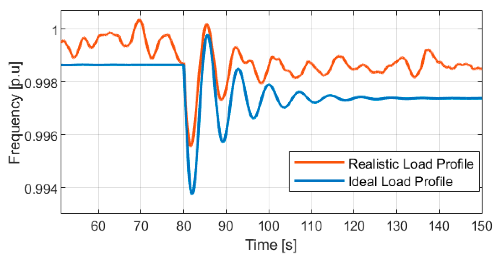
  • The proposed estimation method, has very high accuracy. It is demonstrated that, in real-world scenarios with stochastic load variations, the estimation still works with an estimation error of less than 1%.
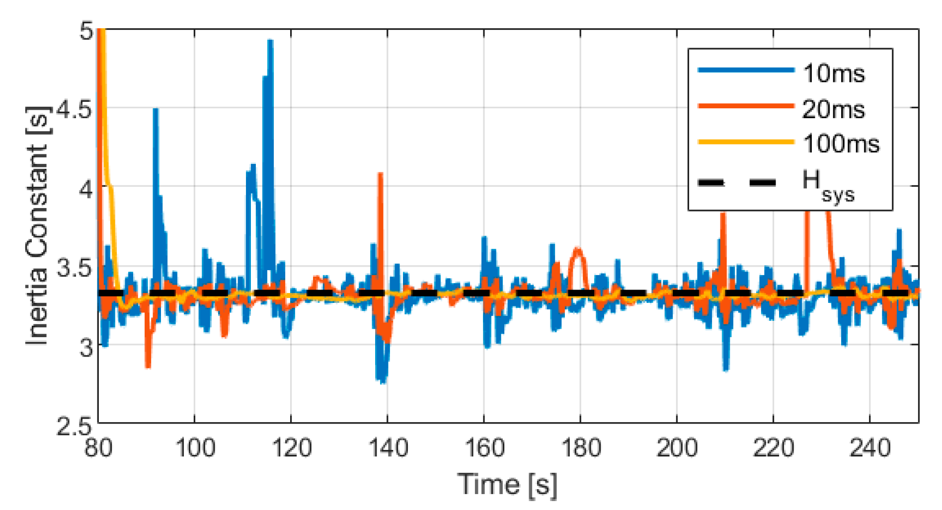
  • The estimation method can be applied during normal operation and hence it can provide continuous online estimations.
  • The estimation method can be used for identifying the inertia and damping coefficients of both SGs and converter-interfaced generation with high accuracy. The estimation errors are less than 0.5% and 3% for SGs and converter-interfaced generation, respectively.
  • The estimation method successfully estimates the amount of virtual inertia provided by the low-pass filter used in droop controllers. This result confirms the relationship between droop controllers and VSM and shows that the swing equation can be used for modelling the droop control. Furthermore, additional control parameters can be identified, i.e., using Equation (13), the cut-off frequency of the low pass filter of the converter can be calculated.
  • The proposed approach eliminates the impact of damping, including PFC and FFR, on the accuracy of inertia estimation. Hence, the knowledge of PFC and FFR models is not required.
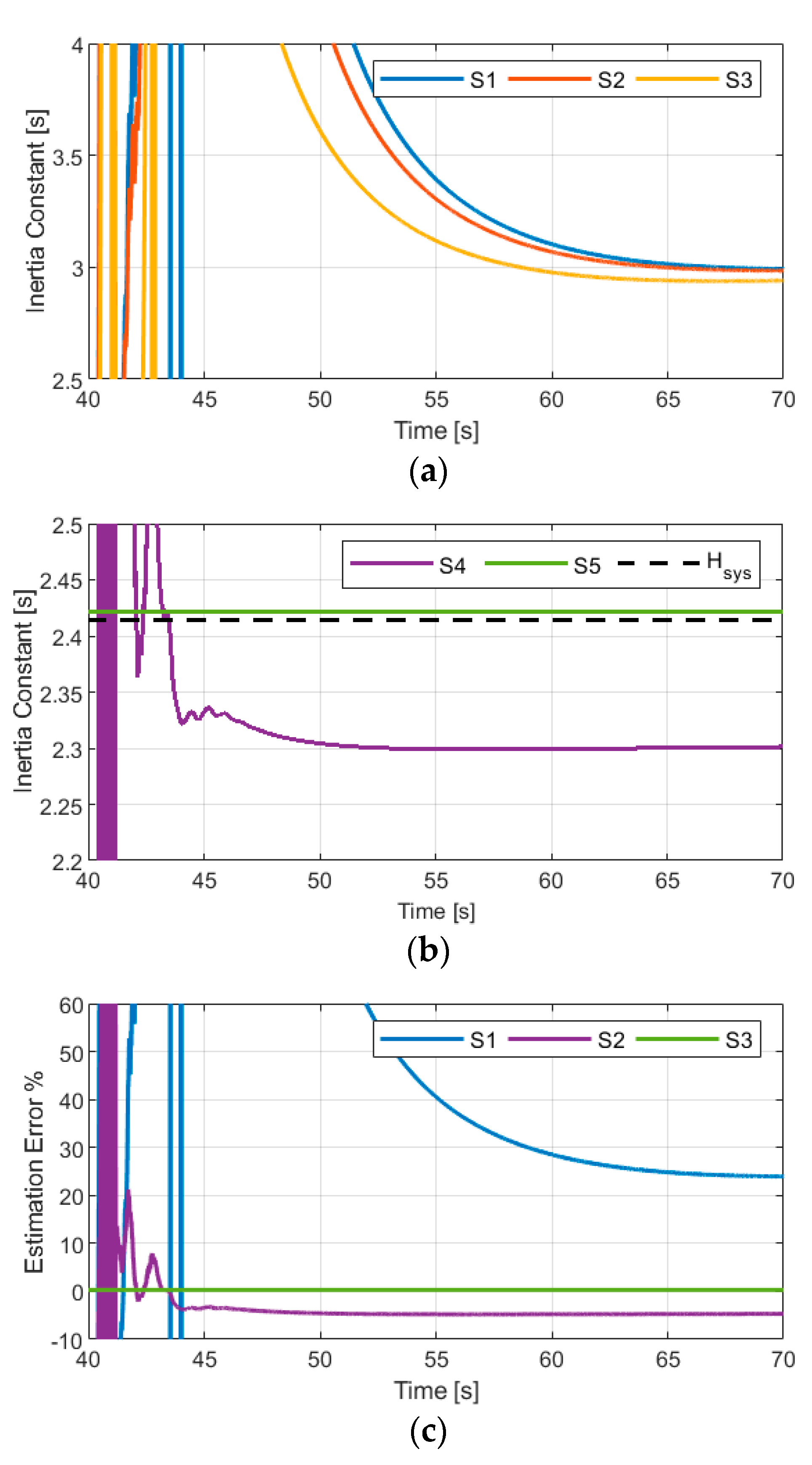
  • When it comes to systems with heterogeneous inertia, estimating the overall system inertia at the system level results in large estimation errors. Hence, it is crucial to estimate the local inertia at an area level. This approach would be desirable by SOs not only to achieve accurate estimation results but also because the local inertia values per area are needed for protective actions and regional ancillary markets. Moreover, a distributed approach, considerably reduces the amount of data that needs to be centrally processed.
  • The time scale difference between FFR and PFC affects the convergence time of the inertia estimation of systems with mixed generation.
  • The inertia estimation accuracy can be further improved by performing the estimation at a machine level, in contrast to at an area level, and then calculate the overall system inertia.
  • The timescale difference between the FFR and PFC affects the damping coefficient estimation accuracy. Hence, for the damping coefficient estimation it is crucial to either perform the estimation per area with resources of similar control timescales or in case the knowledge of the PFC models is available, include the PFC models into the parameterization and estimate the damping resulting from the faster controls, i.e., converter-interfaced generation.
Future work envisages the extension of the proposed work to include further analysis on turbine dynamic heterogeneity and the PFC dead-band. Other compelling directions for future work are to investigate the effect of real-world measurement resolution, uncertainty, and noise on the estimation performance.

Author Contributions

Conceptualization, D.N.; Methodology, D.N.; Software, D.N.; Validation, D.N.; Formal Analysis, D.N.; Writing—Original Draft Preparation, D.N.; Writing—Review and Editing, F.P.; Visualization, D.N.; Supervision, F.P. and A.M.; Project Administration, A.M.; Funding Acquisition, A.M. All authors have read and agreed to the published version of the manuscript.

Funding

This work has been undertaken within the framework of the European Union’s Horizon 2020 research and innovation program under IELECTRIX project grant agreement No. 824392 and edgeFLEX project grant agreement No. 883710.

Conflicts of Interest

The authors declare no conflict of interest.

References

  1. Ulbig, A.; Borsche, T.S.; Andersson, G. Impact of Low Rotational Inertia on Power System Stability and Operation. IFAC Proc. 2014, 47, 7290–7297. [Google Scholar] [CrossRef] [Green Version]
  2. ENTSO-E. Fast Frequency Reserve—Solution to the Nordic Inertia Challenge. Available online: https://www.fingrid.fi/globalassets/dokumentit/fi/sahkomarkkinat/reservit/fast-frequency-reserve-solution-to-the-nordic-inertia-challenge.pdf (accessed on 16 August 2021).
  3. ENTSO-E. Future System Inertia. 2018. Available online: https://eepublicdownloads.entsoe.eu/clean-documents/Publications/SOC/Nordic/Nordic_report_Future_System_Inertia.pdf (accessed on 16 August 2021).
  4. Cai, G.; Wang, B.; Yang, D.; Sun, Z.; Wang, L. Inertia Estimation Based on Observed Electromechanical Oscillation Response for Power Systems. IEEE Trans. Power Syst. 2019, 34, 4291–4299. [Google Scholar] [CrossRef]
  5. Wall, P.; Gonzalez-Longatt, F.; Terzija, V. Estimation of generator inertia available during a disturbance. In Proceedings of the 2012 IEEE Power and Energy Society General Meeting, San Diego, CA, USA, 22–26 July 2012. [Google Scholar] [CrossRef]
  6. Ashton, P.M.; Taylor, G.A.; Carter, A.M.; Bradley, M.E.; Hung, W. Application of phasor measurement units to estimate power system inertial frequency response. In Proceedings of the 2013 IEEE Power & Energy Society General Meeting, Vancouver, BC, Canada, 21–25 July 2013. [Google Scholar] [CrossRef]
  7. Zografos, D.; Ghandhari, M. Estimation of power system inertia. In Proceedings of the 2016 IEEE Power and Energy Society General Meeting (PESGM), Boston, MA, USA, 17–21 July 2016. [Google Scholar] [CrossRef]
  8. Zografos, D.; Ghandhari, M. Power system inertia estimation by approaching load power change after a disturbance. In Proceedings of the 2017 IEEE Power & Energy Society General Meeting, Chicago, IL, USA, 16–20 July 2017. [Google Scholar] [CrossRef]
  9. Cao, X.; Stephen, B.; Abdulhadi, I.F.; Booth, C.D.; Burt, G.M. Switching Markov Gaussian Models for Dynamic Power System Inertia Estimation. IEEE Trans. Power Syst. 2016, 31, 3394–3403. [Google Scholar] [CrossRef] [Green Version]
  10. Tuttelberg, K.; Kilter, J.; Wilson, D.; Uhlen, K. Estimation of Power System Inertia from Ambient Wide Area Measurements. IEEE Trans. Power Syst. 2018, 33, 7249–7257. [Google Scholar] [CrossRef] [Green Version]
  11. Fernández-Guillamón, A.; Vigueras-Rodríguez, A.; Molina-Garcia, Á. Analysis of power system inertia estimation in high wind power plant integration scenarios. IET Renew. Power Gener. 2019, 13, 2807–2816. [Google Scholar] [CrossRef]
  12. H2020n Migrate Project. Deliverable D2.1 Requirements for Monitoring & Forecasting PE-Based KPIs. Available online: https://www.h2020-migrate.eu/_Resources/Persistent/7c5fc3e4d17b17ca2e3ea78815bfd35998cf2ae0/D2.1%20-%20Requirements%20for%20Monitoring%20and%20Forecasting%20PE-based%20KPIs.pdf (accessed on 16 August 2021).
  13. Liu, M.; Chen, J.; Milano, F. On-Line Inertia Estimation for Synchronous and Non-Synchronous Devices. IEEE Trans. Power Syst. 2021, 36, 2693–2701. [Google Scholar] [CrossRef]
  14. Schiffer, J.; Aristidou, P.; Ortega, R. Online Estimation of Power System Inertia Using Dynamic Regressor Extension and Mixing. IEEE Trans. Power Syst. 2019, 34, 4993–5001. [Google Scholar] [CrossRef] [Green Version]
  15. Andersson, G. Dynamics and Control of Electric Power Systems. Available online: http://citeseerx.ist.psu.edu/viewdoc/download?doi=10.1.1.471.7315&rep=rep1&type=pdf (accessed on 16 August 2021).
  16. Athay, T.; Podmore, R.; Virmani, S. A Practical Method for the Direct Analysis of Transient Stability. IEEE Trans. Power Appar. Syst. 1979, PAS-98, 573–584. [Google Scholar] [CrossRef]
  17. Derviškadić, A.; Zuo, Y.; Frigo, G.; Paolone, M. Under Frequency Load Shedding based on PMU Estimates of Frequency and ROCOF. In Proceedings of the 2018 IEEE PES Innovative Smart Grid Technologies Conference Europe (ISGT-Europe), Sarajevo, Bosnia and Herzegovina, 21–25 October 2018. [Google Scholar] [CrossRef] [Green Version]
  18. Beltran, O.; Peña, R.; Segundo, J.; Esparza, A.; Muljadi, E.; Wenzhong, D. Inertia Estimation of Wind Power Plants Based on the Swing Equation and Phasor Measurement Units. Appl. Sci. 2018, 8, 2413. [Google Scholar] [CrossRef] [Green Version]
  19. D’Arco, S.; Suul, J.A. Virtual synchronous machines—Classification of implementations and analysis of equivalence to droop controllers for microgrids. In Proceedings of the 2013 IEEE Grenoble Conference, Grenoble, France, 16–20 June 2013. [Google Scholar] [CrossRef]
Figure 1. IEEE 39-bus New England test system. The base case system presented in (a) constitutes only synchoronous generators. The modified system in (b) includes converter-interfaced generation, placed at buses 5, 8, 9 and 10.
Energies 14 05047 g001
Figure 2. The average frequency of the system with different load profiles following a load step.
Energies 14 05047 g002
Figure 3. The inertia estimation performance under different load profiles in terms of (a) the estimated total inertia constant and (b) the relative estimation error of the actual total inertia constant.
Energies 14 05047 g003
Figure 4. The trajectory of the estimated inertia during normal operation for different measurement time resolutions.
Energies 14 05047 g004
Figure 5. Comparison of the inertia estimation performance of systems with mixed generation: (a) the estimated total inertia constant in scenarios S1, S2 and S3; (b) the estimated total inertia constant in scenarios S4 and S5; (c) the relative estimation error of the total inertia constant in systems with mixed generation.
Energies 14 05047 g005
Figure 6. Comparison of the system unweighted average frequency, COI frequency and the average frequency in different areas of the system following a load step at bus 36.
Energies 14 05047 g006
Figure 7. The impact of parameterization on the damping coefficient estimation: (a) comparison of the effect of parameterization on the damping estimation in Area 2 of the 39-bus system; (b) comparison of the overall system damping under different scenarios.
Energies 14 05047 g007
Table 1. The IEEE 39-bus System Synchronous Generators Inertia Constants.
GeneratorInertia
Constant H (s)
GeneratorInertia
Constant H (s)
SG15SG63.48
SG23.03SG72.64
SG33.58SG82.43
SG42.86SG93.45
SG52.6SG104.2
Table 2. Estimated inertia and damping at the machine level.
MachineEstimated
Inertia
Constant H (s)
Relative
Estimation
Error
Estimated Damping Coefficient
D (p.u)
Relative
Estimation
Error
SG15.01270.25%19.9579−0.21%
SG23.0162−0.46%19.9386−0.0031%
SG33.58560.16%19.9966−0.017%
SG42.86590.21%19.9962−0.015%
VSM52.61870.72%19.5195−2.40%
SG63.48650.19%19.9987−0.007%
SG72.64690.26%19.9994−0.003%
Droop80.32752.91%19.8112−0.94%
Droop90.32752.91%18.6245−6.88%
Droop100.32752.91%19.9257−0.37%
Table 3. Summary of the different scenarios used for estimating the overall inertia of systems with mixed generation.
ScenarioInertia Estimation MannerFFR Parameters KnownPFC Parameters Known
S1at system levelXX
S2at system level X
S3at system level
S4at area levelXX
S5at machine level
Table 4. System inertia constant estimation errors for different estimation scenarios.
ScenarioInertia Constant Estimation Error
S123.96%
S223.45%
S321.80%
S44.69%
S50.29%
Publisher’s Note: MDPI stays neutral with regard to jurisdictional claims in published maps and institutional affiliations.

