Article

Application of Surrogate Optimization Routine with Clustering Technique for Optimal Design of an Induction Motor

Department of Electrical Engineering and Automation, Aalto University, 02150 Espoo, Finland
*
Authors to whom correspondence should be addressed.
Energies 2021, 14(16), 5042; https://doi.org/10.3390/en14165042
Submission received: 8 July 2021 / Revised: 6 August 2021 / Accepted: 13 August 2021 / Published: 17 August 2021
(This article belongs to the Special Issue Magnetic Material Modelling of Electrical Machines)

Abstract

:
This paper proposes a new surrogate optimization routine for optimal design of a direct on line (DOL) squirrel cage induction motor. The geometry of the motor is optimized to maximize its electromagnetic efficiency while respecting the constraints, such as output power and power factor. The routine uses the methodologies of Latin-hypercube sampling, a clustering technique and a Box–Behnken design for improving the accuracy of the surrogate model while efficiently utilizing the computational resources. The global search-based particle swarm optimization (PSO) algorithm is used for optimizing the surrogate model and the pattern search algorithm is used for fine-tuning the surrogate optimal solution. The proposed surrogate optimization routine achieved an optimal design with an electromagnetic efficiency of 93.90 % , for a 7.5 kW motor. To benchmark the performance of the surrogate optimization routine, a comparative analysis was carried out with a direct optimization routine that uses a finite element method (FEM)-based machine model as a cost function.

1. Introduction

Electrical machines have a wide range of use cases, from household utilities to industrial applications, which consume a huge share of all the generated electrical energy [1]. To reduce the global greenhouse gas emissions, it is important to design electrical machines with high energy efficiency. The characteristics of the electrical machines are usually analyzed with a finite element method (FEM)-based electromagnetic simulation for better accuracy. The output characteristics of the electrical machine are highly sensitive to the design variables and the global search optimization algorithms, such as particle swarm optimization (PSO) or genetic algorithm (GA), require many model evaluations to reach the desired optimal solution [2,3]. This causes the optimization process with a FEM-based machine model as a cost function to be computationally expensive [4]. To utilize the time and computational resources efficiently, surrogate optimization techniques are used to optimize the electrical machines, which requires only a few FEM simulations for evaluation.
Response surface methodology (RSM) is a technique used to develop a polynomial function for a complex FEM-based multi-physics model, which defines the relationship between design variables and the output response of an electrical machine [5,6,7,8,9]. This polynomial model can be used with an optimization algorithm to search for the optimal solution. The Box–Behnken design, one of the popular response surface approaches, is used in conjunction with the FEM-based machine model to generate second-order polynomial functions for objective and constraints of the electrical machine [10,11,12,13,14]. The range of the boundaries of the design variables affect the accuracy of the polynomial function and in turn the optimal solution of the electrical machine.
In this article, a novel surrogate optimization routine is proposed for optimizing a three-phase direct on line (DOL) squirrel cage induction motor. The rotor bars of the induction machine are not skewed for the sake of the demonstration of the surrogate optimization routine. The aim of the new routine is to discretize the problem domain into a number of subdomains for improving the accuracy of the polynomial models for a better search of the optimal solution, while efficiently using the computational resources with a smaller number of FEM simulations. To utilize the full capacity of the computational resource, the routine is programmed in such a way as to handle 15 FEM simulations in parallel. The methodologies used in the optimization process are Latin-hypercube sampling for design of the experiments, a clustering algorithm for dividing the problem domain and a Box–Behnken design as a response surface approach. The particle swarm optimization (PSO) algorithm is used for optimizing the polynomial functions of the response surfaces, while a pattern search algorithm is used for fine-tuning the surrogate optimal solution from the PSO. For the purpose of visualization, the proposed surrogate optimization routine is demonstrated with a simplification of the design problem, leaving three design variables. Validation of the results from the proposed surrogate optimization routine for a multivariate design problem is performed by comparing it to the direct optimization routine, which uses FEM simulation as a cost function.

2. Optimization Problem

The electrical machine analyzed in the optimization problem is a three-phase squirrel cage induction motor for a direct online industrial application. The electrical steel core material used in the motor is M400-50A and the rotor cage is made of aluminum. The goal of the optimization problem is to maximize the electromagnetic efficiency, η , satisfying the constraints of the output power, P out , and power factor, P F , for a given volume of the machine. The outer diameter of the stator, D se , and axial length of the machine, l, are fixed so that the volume of the machine remains constant throughout the optimization process. The rotor end-ring overhang length, l oh , is kept constant so that the cross-section area of the end ring depends only on the height of the rotor slot. The specifications and fixed parameters of the induction motor for the optimization problem are shown in Table 1. The objective and constraints of the optimization problem are specified in Table 2. The optimization variables and their ranges for the induction motor are shown in Figure 1 and Table 3. The analysis of the machine design is done with timestepping simulation of a 2D finite element solver software, FCSMEK, developed by the research group of electromechanics at Aalto university [15]. The simulation of the timestepping analysis computes the electromagnetic characteristics of electrical machines by solving the circuit and field equations with the Crank–Nicholson timestepping method. The time is discretized at short time intervals and the magnetic field, currents, and potentials of the windings are solved at successive instants of time. The rotation of the rotor is accomplished by changing the finite element mesh in the air gap. The non-linear system of equations obtained at each timestep is solved using the Newton–Raphson method. The core losses are evaluated using the modified Jordan loss equation with a two-component loss model, namely with eddy current loss and hysteresis loss. The excess losses are included in the dynamic eddy current loss computation [15]. For simplicity, the mechanical losses and other manufacturing losses are not considered for comparing the results of the optimal solutions. Hence, the electromagnetic efficiency η is computed as shown in Equation (1).
η = P in P elec P in × 100 %
where P in is the input power of the induction motor and P elec is the electromagnetic loss of the induction machine, which is comprised of iron losses and copper losses of the stator and rotor. The steady state temperature of the stator and rotor are considered as 80 °C and 100 °C, respectively, for the simulation.

3. Response Surface Methodology Optimization with Box–Behnken Design

Response surface methodology (RSM) is a set of mathematical and statistical techniques used to draw a relationship between control variables (inputs) and output response. This relationship can be approximated into a polynomial model, which can be useful in predicting the response of the control variables, hypothesis testing and finding the optimal condition of the variable settings [16]. In practice, the response surface methodology can be applied to simulate experimental results or for constructing a surrogate function of a computationally expensive multi-physics model. Optimizing the geometric variables of the induction motor directly with the finite element model is computationally expensive. In this article, for boundary-constrained input variables the RSM is used for approximating the electrical quantities of an induction machine into a second-order polynomial model. The second-order polynomial model that describes the functional relationship of the RSM between the control variables and the output response is as shown in Equation (2) [17].
y = β 0 + i = 1 k β i x i + i = 1 k β i i x i 2 + i = 1 k 1 j = i + 1 k β i j x i x j
where y is the output response, x i and x j are the input control variables, β 0 , β i , β i i , a n d β i j are the coefficients of the input control variable terms, and k is the number of control variables. The coefficients are estimated as shown in Equation (3).
β = [ X T X ] 1 X T Y
where X is the matrix of input control variables sampled at multiple points and Y is the corresponding output response vector. The surrogate function shown in Equation (2) works well for interpolation of design variables to predict the output response, but prediction of output response by extrapolation of design variables can be inaccurate. One of the commonly used designs for determining the response surface, as shown in Equation (2), is the Box–Behnken design codeveloped by Box and Behnken in 1960 [18]. If the control variable space is defined as a cube, then the sample points are taken at the geometric center of the cube and at the middle points of the edges of the cube. The Box–Behnken design sample points represented for a three-dimensional control variable space are shown in Figure 2. Positioning sample points in this way preserves a uniform variance within the definition of the hyper-cube [18]. The number of sample points, N, for a given number of control variables is shown in Equation (4) [19].
N = 2 k ( k 1 ) + C 0
where k is the number of design variables and C 0 is the number of center points.
The Box–Behnken design was applied to the problem of an induction machine as described in Section 2 for performing the surrogate optimization. The process flow of optimization with the Box–Behnken design is presented in Figure 3. For easier representation, the optimization variables presented in Table 3 are assumed as x 1 , x 2 , x 3 , x 8 in their respective order. Based on the optimization variable boundaries from Table 3, the Box–Behnken design sample points were created for the variables as an eight-dimensional hypercube. These samples were simulated with FCSMEK finite element software for calculating their corresponding response characteristics, such as efficiency, η , output power, P out , and power factor, P F . The relationship between the optimization variables and the output response was established as a second-order polynomial function as shown in Equation (2). The coefficients of the polynomial terms were calculated from the predetermined output responses by FEM simulations sampled at Box–Behnken sample points as shown in Equation (3). The polynomial response functions for the surrogate optimization problem are presented in Appendix A. These surrogate functions were used as the cost function of the PSO algorithm. A population of 1000 particles of the PSO was initialized with the Latin-hypercube sampling method.
The objective and constraints of the problem are as shown in Table 2. The optimal motor design from Box–Behnken design is validated with FEM simulation as shown in Table 4. It is observed that a difference in the result of the objective electromagnetic efficiency, η , between the surrogate optima and its FEM validation is considerably high. Moreover, the optimal solution does not respect the constraints of the output power, P out , and the power factor, P F , coupled with a high margin of error. The accuracy of the surrogate functions is impacted by the application of the Box–Behnken design to a large design variable space. Hence, a new optimization routine is proposed in this article (Section 6) for improving the accuracy of the surrogate functions resulting in an improved optimal solution.

4. Latin-Hypercube Sampling

Latin-hypercube sampling is a statistical method for selecting near-random samples from the input variable space, proposed by McKay, Beckman, and Conover [20]. It uses a sampling scheme of stratification to improve the distribution of samples in the input variable space. To select n Latin-hypercube samples for a sampling function with x i = ( x 1 , x 2 ) as input variables, the range of each of the x i is stratified into n equiprobable intervals. One observation is selected at random from each of the n intervals. These observations corresponding to x 1 and x 2 are matched at random to form n Latin-hypercube samples. A set of five samples generated with the Latin-hypercube sampling method for the input variables of x i = ( x 1 , x 2 ) is shown in Figure 4. The Latin-hypercube sampling method is widely used in the design of experiments for various applications of computer modeling [21,22,23]. In this article, the Latin-hypercube sampling method is used in the proposed optimization routine for selecting samples that satisfy a set of criteria and for initializing the first swarm of the PSO algorithm.

5. Clustering

Clustering is a method involved in partitioning a given dataset into different groups or clusters. The data that are mapped to a particular cluster tend to have similar characteristics and follow a similar pattern [24]. Clustering helps in classifying and analyzing large datasets, which can be applied in fields of machine learning, data science, pattern recognition, image processing, and bioinformatics [25,26,27]. The k-means is one of the oldest computational techniques used in solving clustering problems, based on the algorithm proposed by Lloyd [28]. If an integer k is chosen for partitioning a dataset into k clusters and n is the number of data points of the dataset, the goal of Lloyd’s (k-means) algorithm is to find k centroids so as to minimize the potential function, γ . The potential function γ is a measure of the total squared Euclidean distance between each data point and its closest centroid, as shown in Equation (5).
γ = j = 1 k i = 1 m x i + c j 2
where m is the number of data points in the jth cluster, x i and c j are the data points and centroid of the jth cluster. Since Lloyd’s (k-means) algorithm involves selecting the initial k centroids uniformly at random from the dataset, it suffers from inconsistency and accuracy issues. Arthur and Vassilvitskii proposed a randomized seeding technique for selecting the initial centroids of the k-means and combined it with the original k-means algorithm to call it the k-means++ algorithm with improved speed and accuracy [29]. A set of randomly generated samples clustered with the k-means++ algorithm is shown in Figure 5. In the proposed surrogate optimization routine, the k-means++ algorithm is used in partitioning the samples created from design variables into different clusters. In a multi-variable clustering problem, the variables can have varying scales of magnitude and incomparable units. Thus, it is required to apply the feature scaling technique to normalize the data for standardization. Z-score transformation is one of the successful standardization techniques utilized before applying the k-means clustering method to a dataset [30]. Equation (6) is used to estimate the Z-score,
x = x x ¯ σ x
where x is the variable vector that needs to be standardized, x ¯ and σ x are the mean and standard deviation of the vector x , and x is the transformed variable vector that implies the z-score.

6. The Proposed Surrogate Optimization Routine

To overcome the issue in the accuracy of the surrogate model as shown in Section 3, a new surrogate optimization routine is proposed for the induction machine problem. The concepts of Latin-hypercube sampling, clustering, and Box–Behnken design are used in the proposed optimization routine, and algorithms such as PSO and pattern search are used for optimizing the control variables of the problem statement. The proposed optimization routine is divided into two parts, namely a surrogate optimization part and a pattern search part, which are presented as flow charts in Figure 6 and Figure 7, respectively. The implementation of the surrogate optimization routine was carried out with MATLAB programming.
The surrogate optimization part begins with the design of experiments using the Latin-hypercube sampling method. The design variables shown in Table 3 were sampled for 500 Latin-hypercube samples within the boundaries of the variable design space. These samples were simulated with FCSMEK finite element software for calculating their output responses, including electromagnetic efficiency, η , output power, P out , and power factor, P F . A set of criteria (satisfying the threshold values of the output responses) was devised to select a set of samples from the design of experiment. The design variables of the selected samples were standardized as shown in Equation (6), and clustered with the k-means ++ algorithm into different groups or clusters. The optimality of the number of clusters was evaluated by the MATLAB built-in function e v a l c l u s t e r s using the gap statistics criterion [31,32]. The domain of the optimization problem was divided into n clusters and within those clusters, new boundaries of the design variables were established. The surrogate optimization process with Box–Behnken design as explained in Section 3 was applied to each cluster. At the end of the surrogate optimization, n surrogate optimal solutions were obtained. The accuracy of the surrogate optimal solutions was validated with timestepping FEM simulation.
The surrogate optimal solutions were used for initializing the pattern search optimization algorithm. The goal of the pattern search algorithm is to search for an optimal solution in the vicinity of the surrogate optimal solution, which improves the objective of the optimization problem while respecting the constraints. The FEM simulation was used as a cost function for the pattern search algorithm. The final improved optimal solution was obtained at the end of the pattern search optimization process.

7. Results

7.1. Visualization of a 3-Variable Optimization

A three-variable optimization problem for an induction machine is demonstrated to visualize the flow of the proposed surrogate optimization routine as shown in Figure 8. The stator inner diameter, D s , stator yoke width, h ys , and slip, s, from Table 3 were chosen as the design variables and the remaining variables were fixed to constant values. The objective and constraints of the optimization problem are presented in Table 2. A set of 500 samples of the optimization variables were generated using the Latin-hypercube sampling method as shown in Figure 8a. These samples were simulated with FCSMEK finite element software to calculate the respective output responses. Selection criteria based on the output response of the samples as presented in Table 5 were applied to the Latin-hypercube samples to pick the samples of interest, as shown in Figure 8b. These samples were clustered into different groups as shown in Figure 8c. The Box–Behnken domain of each of the groups was as shown in Figure 8d. The surrogate optimal solution was computed and validated with FEM simulation for each of the clusters. The best solution of the surrogate optimization from one of the clusters is presented in Table 6. It is seen that the difference in the computation of the surrogate optimal solution has been reduced considerably when compared with the results from Table 4, but the constraint of the output power P out is not respected. The pattern search algorithm with FEM simulation as the cost function was applied to the surrogate optimal solution to search for a better solution in its vicinity. The objective and design variables of the optimal solution from the surrogate optimization part and pattern search part are compared in Table 7 and Table 8. It can be seen that the pattern search algorithm found a marginally better solution in the neighborhood of the surrogate optimal solution, while respecting the constraints of the optimization problem. The electromagnetic efficiency, power factor and electromagnetic losses are compared for various load points in Table 9 and Table 10.

7.2. Multivariate Optimization

The proposed surrogate optimization routine was applied to a multivariate optimization problem as specified in Section 2. The selection criteria of the samples based on its output response for the clustering process were as shown in Table 5. The output response of the surrogate optimal solution from one of the clusters was validated with FEM simulation as presented in Table 11. It was found that difference in the output responses has been reduced considerably when compared with the solution presented in Table 4. The decrease in difference of the output response leads to the surrogate optimal solution respecting the set of constraints of the optimization problem. The pattern search algorithm improves the objective of the surrogate optimal solution by searching in the vicinity of the surrogate design. The objective and design variables at the end of both the surrogate optimal part and the pattern search part are compared in Table 12 and Table 13. It can be noted from Table 13 that to improve the electromagnetic efficiency, η , of the surrogate optimal solution, the values of the design variables, such as air gap width, δ , stator tooth width, b ds , and stator yoke width, h ys , have changed by a small margin. The electromagnetic efficiency, power factor, and electromagnetic losses are compared for various load points in Table 14 and Table 15. The flux density distribution of the optimal solution (quadrant of the optimal induction machine) at the end of pattern search algorithm is shown in Figure 9.

7.3. Comparison: Proposed Surrogate Optimization Routine vs. Direct Optimization Routine

In this section, the result from the proposed surrogate optimization routine is compared with the direct optimization routine, which uses FEM simulation as the cost function. The flow chart of the direct optimization routine is presented in Figure 10. The computational cost of the direct optimization routine is high since it uses FEM simulation as the cost function. The PSO algorithm and pattern search algorithm were used in the direct optimization routine with the same configuration as that of the proposed surrogate optimization routine. Due to the high computational cost of the FEM simulation and limitation in the computational capabilities of the research workstation, the size of the population was fixed to 30 particles for the PSO algorithm in the direct optimization routine. The optimal solution from the PSO algorithm was used to initialize the pattern search algorithm, which searches for a better solution in the vicinity. The objective and design variables of the optimal solution from the proposed surrogate optimization routine are compared with the optimal solution from the direct optimization routine in Table 16 and Table 17. The electromagnetic efficiency, η , of the optimal solution from the proposed surrogate optimization routine reached closer to that of the direct optimization routine. The marginal difference in the design variables slip, s, rotor slot lower width, b 5 r , and rotor yoke width, h yr , between the routines impacts the electromagnetic efficiency, η , of the optimal solutions. The electromagnetic efficiency, power factor, and electromagnetic losses are compared for various load points in Table 18 and Table 19. The advantage of using the proposed surrogate optimization routine is that it requires far fewer FEM simulations than the direct optimization routine, while maintaining an accurate evaluation of the optimal design. The optimization routines were performed in the computer with dual processors of Intel Xeon Silver 4114 CPU at a clock-rate of 2.2 GHz, which can handle parallel computations of 15 FEM simulations. The comparison of the number of FEM simulations in the proposed surrogate optimization routine and direct optimization routine is presented in Table 20.
The reliability of the proposed surrogate optimization routine for the induction machine problem was assessed with 20 continuous runs. The electromagnetic efficiency, η , output power, P out , and power factor, P F , of the optimal solution from each run were analyzed to provide the probability distribution as presented in Figure 11. It can be seen that all of the optimal solutions from the proposed surrogate optimization routine respect the constraints specified in the optimization problem and that the range of the objective, electromagnetic efficiency, η , varies between 93.75% and 93.95%.

8. Conclusions

This paper proposes a novel, efficient, and reliable surrogate optimization routine that can be applied to multiple design problems. The proposed clustering technique used in the routine enables improving the accuracy of the surrogate model while exploring promising subsets of the design variable range. The surrogate optimization routine was applied to design an optimal three-phase induction motor, maximizing its efficiency for a given volume. The surrogate functions of the electromagnetic efficiency, output power, and power factor were constructed as a function of eight design variables and these functions acted as the objective and constraints of the optimization problem. A precision of 0.01 mm was considered for the optimization process, which is possible only with laser cutting of the electrical sheets at the prototyping level. A three-variable optimization problem was performed to demonstrate the discretization of the optimization problem into a few sub-domains with the clustering algorithm for searching for the optimal solution. The results of the proposed surrogate optimization routine applied to the multivariate optimization problem show an improved optimal solution when compared with optimization with a simple Box–Behnken design. This proves the improvement of the accuracy of the surrogate functions by the application of the proposed surrogate optimization routine. To benchmark the proposed surrogate optimization routine, a direct optimization routine was applied to the induction motor problem, which uses FEM simulation as a cost function. Upon comparing the results of both routines, the optimal solution from the proposed surrogate optimization routine was shown to reach closer to that from the direct optimization routine. Additionally, the proposed surrogate optimization routine used 1364 FEM simulations compared with 75,208 FEM simulations of the direct optimization routine, thus greatly improving the computational efficiency. Future work on the proposed surrogate optimization routine will focus on performance evaluations on different types of machines and its application for multi-objective optimization problems with several constraints.

Author Contributions

Conceptualization, A.B. (Aswin Balasubramanian); methodology, A.B. (Aswin Balasubramanian), F.M. and A.B. (Anouar Belahcen); software, A.B. (Aswin Balasubramanian), F.M. and A.B. (Anouar Belahcen); validation, A.B. (Aswin Balasubramanian) and F.M.; writing—original draft preparation, A.B. (Aswin Balasubramanian); writing—review and editing, A.B. (Aswin Balasubramanian), F.M., O.O., M.M.B. and A.B. (Anouar Belahcen); visualization, A.B. (Aswin Balasubramanian) and M.M.B.; supervision, A.B. (Anouar Belahcen); project administration, A.B. (Anouar Belahcen); funding acquisition, A.B. (Anouar Belahcen). All authors have read and agreed to the published version of the manuscript.
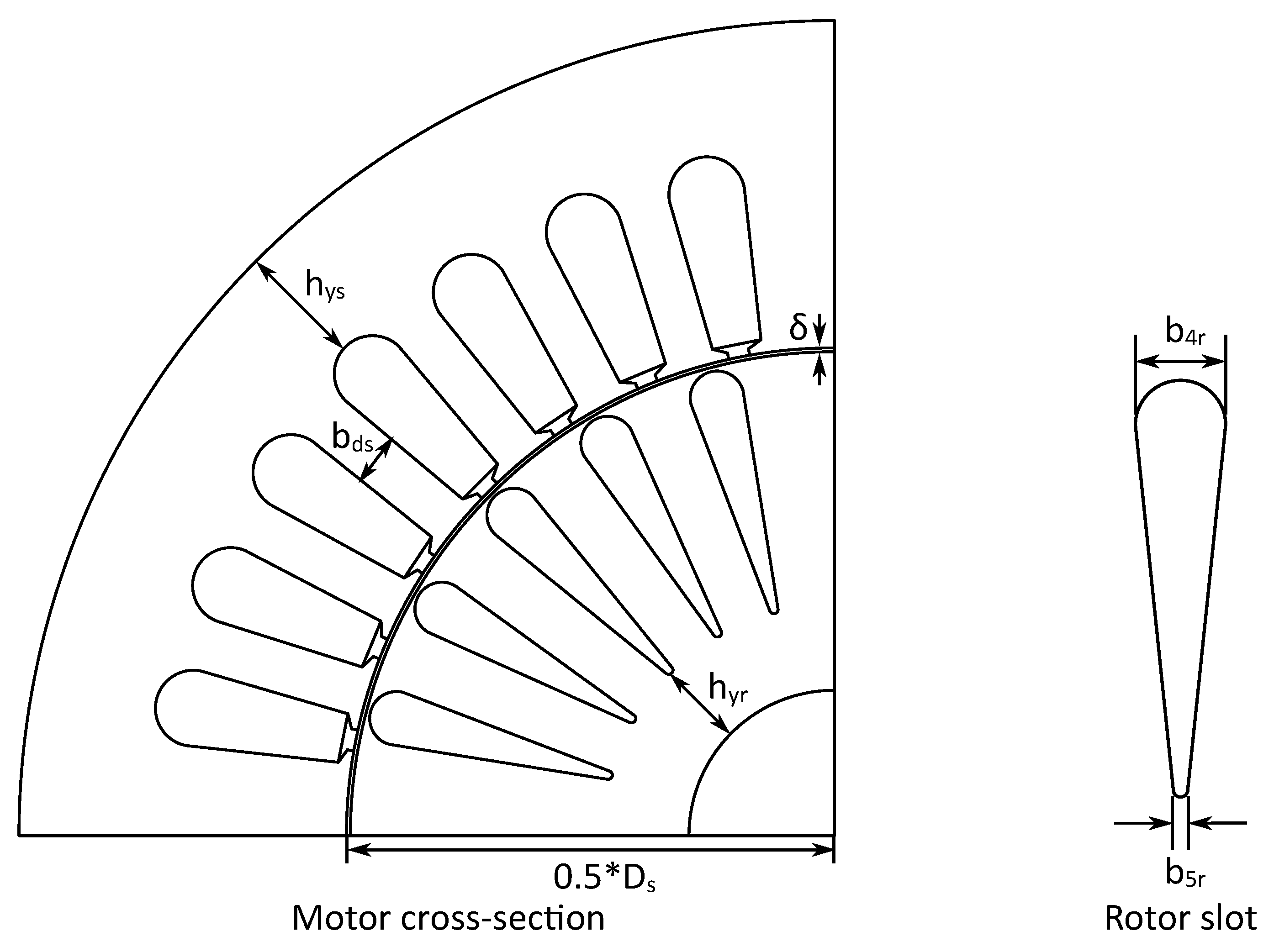
Funding

This work was supported in part by the Academy of Finland consortium grant 330747.

Institutional Review Board Statement

Not applicable.

Informed Consent Statement

Not applicable.

Data Availability Statement

Not applicable.

Acknowledgments

We would like to acknowledge our colleague Alireza Nematsaberi, Department of Electrical Engineering and Automation, Aalto University, for his contribution in brainstorming the idea of this article, and Devi Geetha Nair, R&D Engineer, ABB Oy, Finland for proofreading the article.

Conflicts of Interest

The authors declare no conflict of interest.

Abbreviations

The following abbreviations are used in this manuscript:
DOLDirect On Line
FEMFinite Element Method
PSOParticle Swarm Optimization
GAGenetic Algorithm
RSMResponse Surface Methodology

Appendix A

Table A1. Quadratic closed form equation of Box–Behnken design—constant and first order terms.
Efficiency, η Output Power, P out Power Factor, PF Terms
−2.13−17,793.93−7.21constant
19.70181,583.2045.91 x 1
49.97412,548.7391.53 x 2
33.81−253,121.70114.90 x 3
−66.36−1,451,699.89−1295.93 x 4
54.17−2,003,197.8811.83 x 5
56.87−1,835,156.76176.28 x 6
−14.46−1749.63−47.77 x 7
543.423,068,544.761640.46 x 8
Table A2. Quadratic closed form equation of Box–Behnken design—second-order squared terms.
Efficiency, η Output Power, P out Power Factor, PF Terms
−145.04−13,854,715.08−10,487.18 x 1 2
14092.83203,636,581.33−49,000.00 x 2 2
−2056.07−71,109,777.78−14,800.00 x 3 2
316.60−27,247,703.791164.10 x 4 2
−6796.98−26,223,650.13−14,116.67 x 5 2
1444.9754,209,095.3012,323.08 x 6 2
−4837.02300,328.53−17,066.67 x 7 2
919.65−492,073.973357.69 x 8 2
Table A3. Quadratic closed form equation of Box–Behnken design—second-order product terms.
Efficiency, η Output Power, P out Power Factor, PF Terms
−41.93−745,736.39−135.53 x 1 . x 2
−325.50−2,094,333.11−1541.78 x 1 . x 3
−144.03−2,518,297.47−937.01 x 1 . x 4
−8885.96358,926,619.68−172,724.87 x 1 . x 5
−2609.85−23,720,999.82−16,790.21 x 1 . x 6
−1773.84−96,582,265.11−35,390.48 x 1 . x 7
−81.98−3,469,143.73−878.47 x 1 . x 8
−35253.62−115,771,295.06−143,252.98 x 2 . x 3
−169.52−1,850,886.93−4.83 x 2 . x 4
−101.874,251,893.60−400.60 x 2 . x 5
250.337,026,589.337777.78 x 2 . x 6
80.1120,428,872.871755.56 x 2 . x 7
−212.2214,168,262.83−473.33 x 2 . x 8
51.70964,692.96219.99 x 3 . x 4
−1369.82−12,319,740.72−3271.67 x 3 . x 5
−246.48−1,619,519.09−318.64 x 3 . x 6
397.42−2,404,587.73−5716.67 x 3 . x 7
−550.393,492,065.36−505.00 x 3 . x 8
−377.489,293,965.01−603.33 x 4 . x 5
89.05−1,249,662.46175.38 x 4 . x 6
−2335.66−22,764,991.96−215.00 x 4 . x 7
536.32−1,139,470.0619757.58 x 4 . x 8
−575.7063,834,896.15−2057.58 x 5 . x 6
−431.0448,765,232.48−1333.33 x 5 . x 7
83.45−10,184,611.42237.06 x 5 . x 8
−2747.19−20,314,075.20−4236.36 x 6 . x 7
846.01−91,722,135.1145,777.77 x 6 . x 8
1596.02−106,614,524.4446,888.89 x 7 . x 8

References

  1. Benhaddadi, M.; Olivier, G.; Labrosse, D.; Tetrault, P. Premium efficiency motors and energy saving potential. In Proceedings of the 2009 IEEE International Electric Machines and Drives Conference, Miami, FL, USA, 3–6 May 2009; pp. 1463–1468. [Google Scholar]
  2. Han, W.; Van Dang, C.; Kim, J.W.; Kim, Y.J.; Jung, S.Y. Global-Simplex Optimization Algorithm Applied to FEM-Based Optimal Design of Electric Machine. IEEE Trans. Magn. 2017, 53, 1–4. [Google Scholar] [CrossRef]
  3. Han, W.; Tran, T.T.; Kim, J.W.; Kim, Y.J.; Jung, S.Y. Mass Ionized Particle Optimization Algorithm Applied to Optimal FEA-Based Design of Electric Machine. IEEE Trans. Magn. 2016, 52, 1–4. [Google Scholar] [CrossRef]
  4. Slawomir Wiak, P.; Belahcen, A.; Martin, F.; Zaim, M.E.H.; Dlala, E.; Kolondzovski, Z. Combined FE and Particle Swarm algorithm for optimization of high speed PM synchronous machine. Model. Magn. Electr. Circuits 2015, 34, 475–484. [Google Scholar] [CrossRef]
  5. Jung, J.W.; Lee, B.H.; Kim, K.S.; Kim, S.I. Interior Permanent Magnet Synchronous Motor Design for Eddy Current Loss Reduction in Permanent Magnets to Prevent Irreversible Demagnetization. Energies 2020, 13, 5082. [Google Scholar] [CrossRef]
  6. Ishikawa, T.; Yamada, M.; Kurita, N. Design of Magnet Arrangement in Interior Permanent Magnet Synchronous Motor by Response Surface Methodology in Consideration of Torque and Vibration. IEEE Trans. Magn. 2011, 47, 1290–1293. [Google Scholar] [CrossRef]
  7. Lee, J.H. Optimum Shape Design Solution of Flux Switching Motor Using Response Surface Methodology and New Type Winding. IEEE Trans. Magn. 2012, 48, 1637–1640. [Google Scholar] [CrossRef]
  8. Lee, B.H.; Hong, J.P.; Lee, J.H. Optimum Design Criteria for Maximum Torque and Efficiency of a Line-Start Permanent-Magnet Motor Using Response Surface Methodology and Finite Element Method. IEEE Trans. Magn. 2012, 48, 863–866. [Google Scholar] [CrossRef]
  9. Semon, A.; Melcescu, L.; Craiu, O.; Crăciunescu, A. Design Optimization of the Rotor of a V-type Interior Permanent Magnet Synchronous Motor using Response Surface Methodology. In Proceedings of the 2019 11th International Symposium on Advanced Topics in Electrical Engineering (ATEE), Bucharest, Romania, 28–30 March 2019; pp. 1–4. [Google Scholar]
  10. Lee, S.; Kim, Y.; Lee, K.; Kim, S. Multiobjective Optimization Design of Small-Scale Wind Power Generator With Outer Rotor Based on Box–Behnken Design. IEEE Trans. Appl. Supercond. 2016, 26, 1–5. [Google Scholar] [CrossRef]
  11. Han, J.; Lee, J.; Kim, W. A Study on Optimal Design of the Triangle Type Permanent Magnet in IPMSM Rotor by Using the Box–Behnken Design. IEEE Trans. Magn. 2015, 51, 1–4. [Google Scholar] [CrossRef]
  12. Rafiee, V.; Faiz, J. Robust Design of an Outer Rotor Permanent Magnet Motor Through Six-Sigma Methodology Using Response Surface Surrogate Model. IEEE Trans. Magn. 2019, 55, 1–10. [Google Scholar] [CrossRef]
  13. Bramerdorfer, G. Computationally Efficient Tolerance Analysis of the Cogging Torque of Brushless PMSMs. IEEE Trans. Ind. Appl. 2017, 53, 3387–3393. [Google Scholar] [CrossRef]
  14. Zhu, Z.; Zhu, J.; Zhu, H.; Zhu, X.; Yu, Y. Optimization Design of an Axial Split-Phase Bearingless Flywheel Machine with Magnetic Sleeve and Pole-Shoe Tooth by RSM and DE Algorithm. Energies 2020, 13, 1256. [Google Scholar] [CrossRef] [Green Version]
  15. Arkkio, A. Analysis of Induction Motors Based on the Numerical Solution of the Magnetic Field and Circuit Equations. Ph.D. Thesis, Aalto University, Aalto, Finland, 1987. [Google Scholar]
  16. Khuri, A.I.; Mukhopadhyay, S. Response surface methodology. WIREs Comput. Stat. 2010, 2, 128–149. [Google Scholar] [CrossRef]
  17. Yang, J.; Peterson, J.; Khuri, A.; Goldfarb, H.; Mukhopadhyay, S.; Piepel, G.; Carter, W. Response Surface Methodology And Related Topics; World Scientific Publishing Company: Singapore, 2006. [Google Scholar]
  18. Box, G.E.P.; Behnken, D.W. Some New Three Level Designs for the Study of Quantitative Variables. Technometrics 1960, 2, 455–475. [Google Scholar] [CrossRef]
  19. Zolgharnein, J.; Shahmoradi, A.; Ghasemi, J.B. Comparative study of Box–Behnken, central composite, and Doehlert matrix for multivariate optimization of Pb (II) adsorption onto Robinia tree leaves. J. Chemom. 2013, 27, 12–20. [Google Scholar] [CrossRef]
  20. Mckay, M.D.; Beckman, R.J.; Conover, W.J. A Comparison of Three Methods for Selecting Values of Input Variables in the Analysis of Output From a Computer Code. Technometrics 2000, 42, 55–61. [Google Scholar] [CrossRef]
  21. Przygrodzki, M.; Kubek, P. The Polish Practice of Probabilistic Approach in Power System Development Planning. Energies 2021, 14, 161. [Google Scholar] [CrossRef]
  22. Choi, Y.; Song, D.; Yoon, S.; Koo, J. Comparison of Factorial and Latin Hypercube Sampling Designs for Meta-Models of Building Heating and Cooling Loads. Energies 2021, 14, 512. [Google Scholar] [CrossRef]
  23. Wang, L.; Asomani, S.N.; Yuan, J.; Appiah, D. Geometrical Optimization of Pump-As-Turbine (PAT) Impellers for Enhancing Energy Efficiency with 1-D Theory. Energies 2020, 13, 4120. [Google Scholar] [CrossRef]
  24. Agarwal, P.K.; Mustafa, N.H. K-Means Projective Clustering. In Proceedings of the Twenty-Third ACM SIGMOD-SIGACT-SIGART Symposium on Principles of Database Systems, Paris, France, 14–16 June 2004; Association for Computing Machinery: New York, NY, USA, 2004; pp. 155–165. [Google Scholar]
  25. Chalusiak, M.; Nawrot, W.; Buchaniec, S.; Brus, G. Swarm Intelligence-Based Methodology for Scanning Electron Microscope Image Segmentation of Solid Oxide Fuel Cell Anode. Energies 2021, 14, 3055. [Google Scholar] [CrossRef]
  26. Tadjer, A.; Bratvold, R.B.; Hanea, R.G. Efficient Dimensionality Reduction Methods in Reservoir History Matching. Energies 2021, 14, 3137. [Google Scholar] [CrossRef]
  27. Khan, A.N.; Iqbal, N.; Rizwan, A.; Ahmad, R.; Kim, D.H. An Ensemble Energy Consumption Forecasting Model Based on Spatial-Temporal Clustering Analysis in Residential Buildings. Energies 2021, 14, 3020. [Google Scholar] [CrossRef]
  28. Lloyd, S. Least squares quantization in PCM. IEEE Trans. Inf. Theory 1982, 28, 129–137. [Google Scholar] [CrossRef]
  29. Arthur, D.; Vassilvitskii, S. k-means++: The Advantages of Careful Seeding; Technical Report 2006-13; Stanford InfoLab: Stanford, CA, USA, 2006. [Google Scholar]
  30. Cheadle, C.; Vawter, M.P.; Freed, W.J.; Becker, K.G. Analysis of Microarray Data Using Z Score Transformation. J. Mol. Diagn. 2003, 5, 73–81. [Google Scholar] [CrossRef] [Green Version]
  31. MathWorks. Cluster Visualization and Evaluation. Available online: https://se.mathworks.com/help/stats/cluster-evaluation.html?s_tid=CRUX_topnav (accessed on 1 June 2021).
  32. Tibshirani, R.; Walther, G.; Hastie, T. Estimating the number of clusters in a data set via the gap statistic. J. R. Stat. Soc. Ser. Stat. Methodol. 2001, 63, 411–423. [Google Scholar] [CrossRef]
Figure 1. Optimization variables of the induction motor.
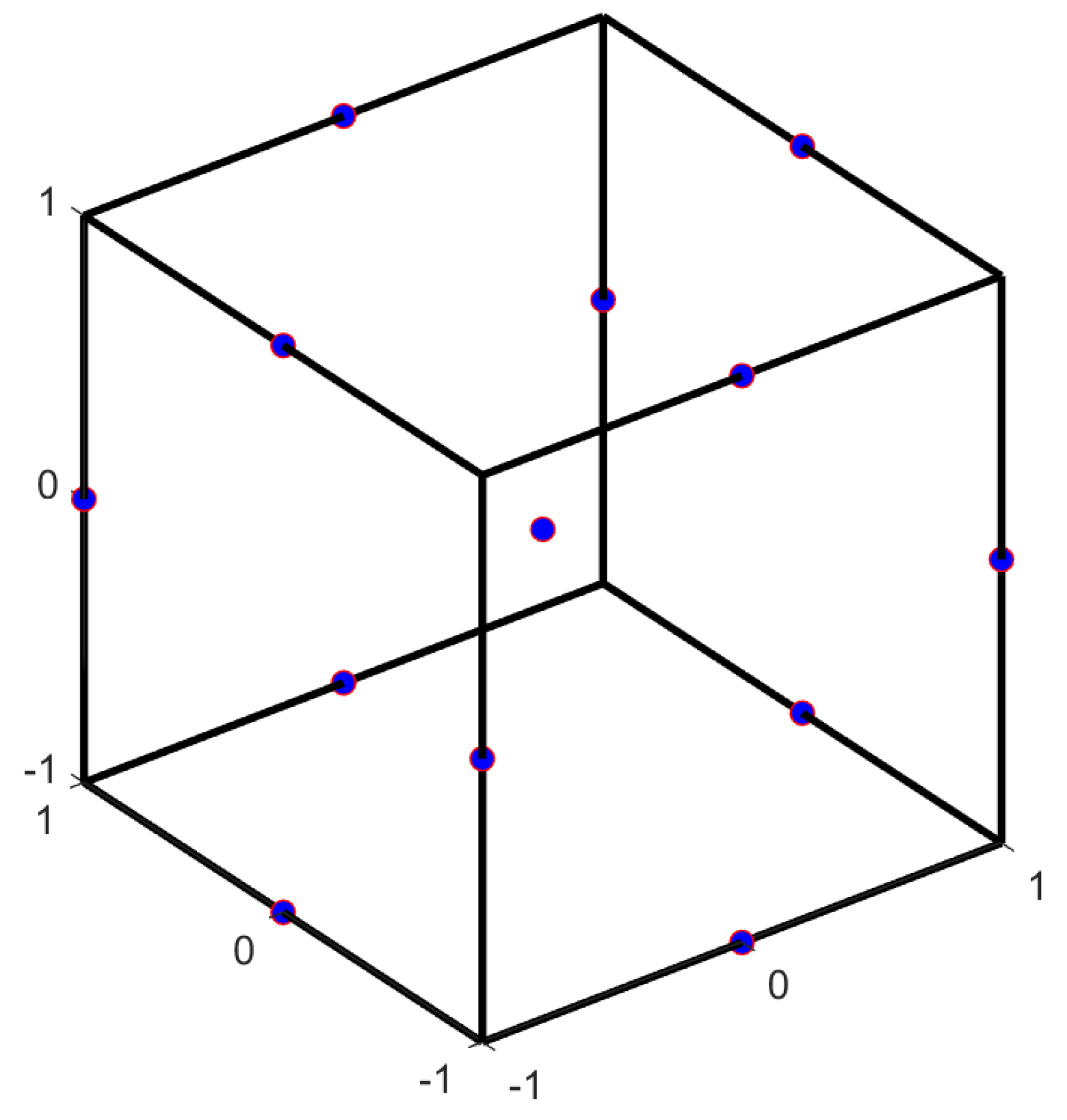
Energies 14 05042 g001
Figure 2. Box–Behnken design represented for a 3-dimensional variable space.
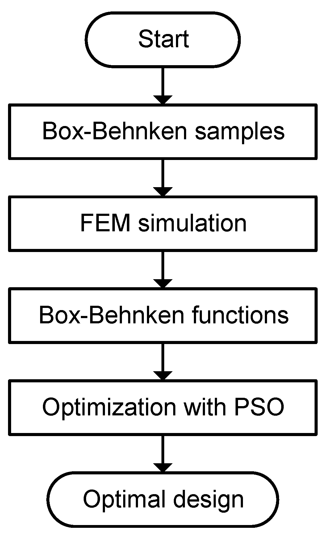
Energies 14 05042 g002
Figure 3. Flow chart: optimization with Box–Behnken design.
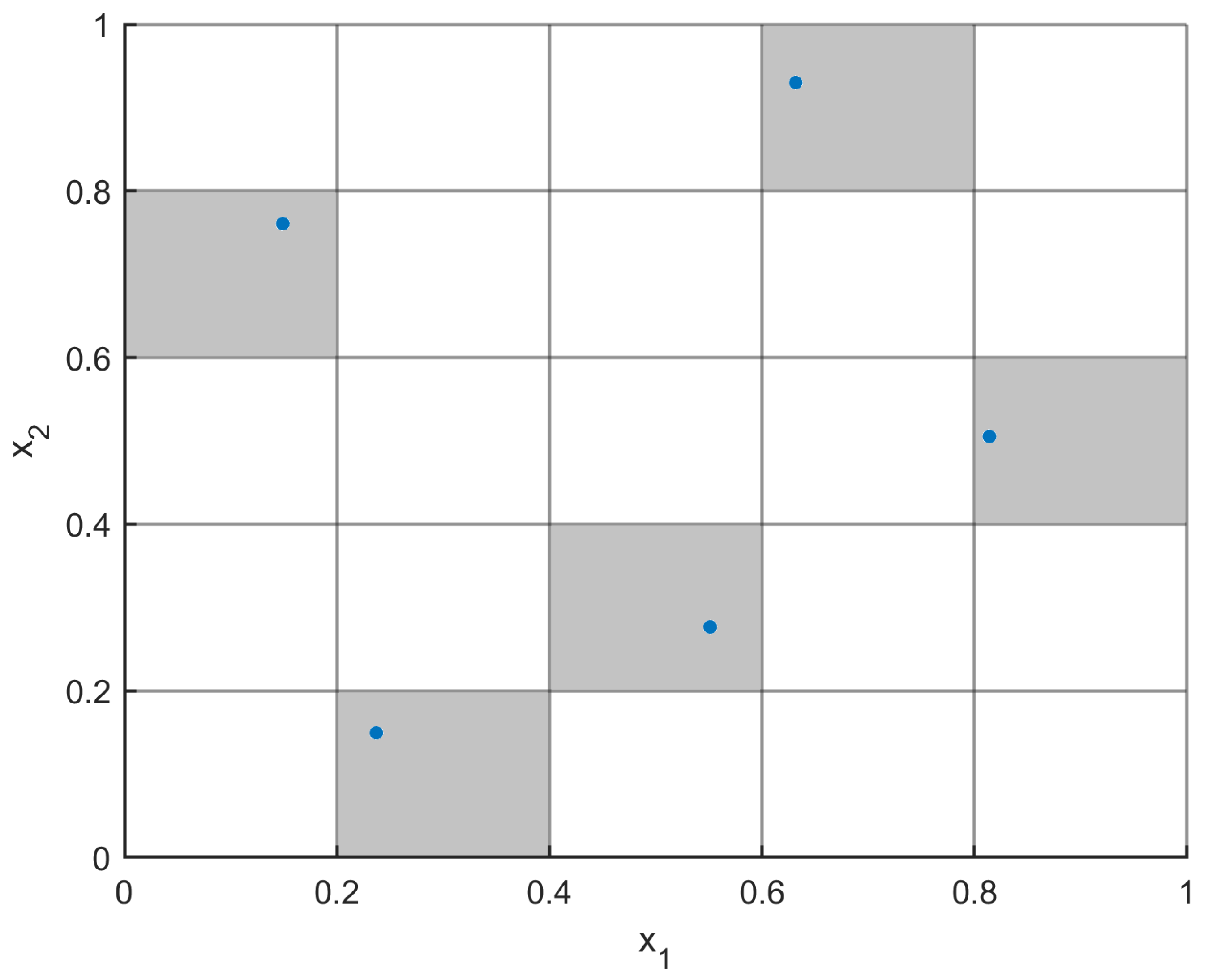
Energies 14 05042 g003
Figure 4. Latin-hypercube sampling.
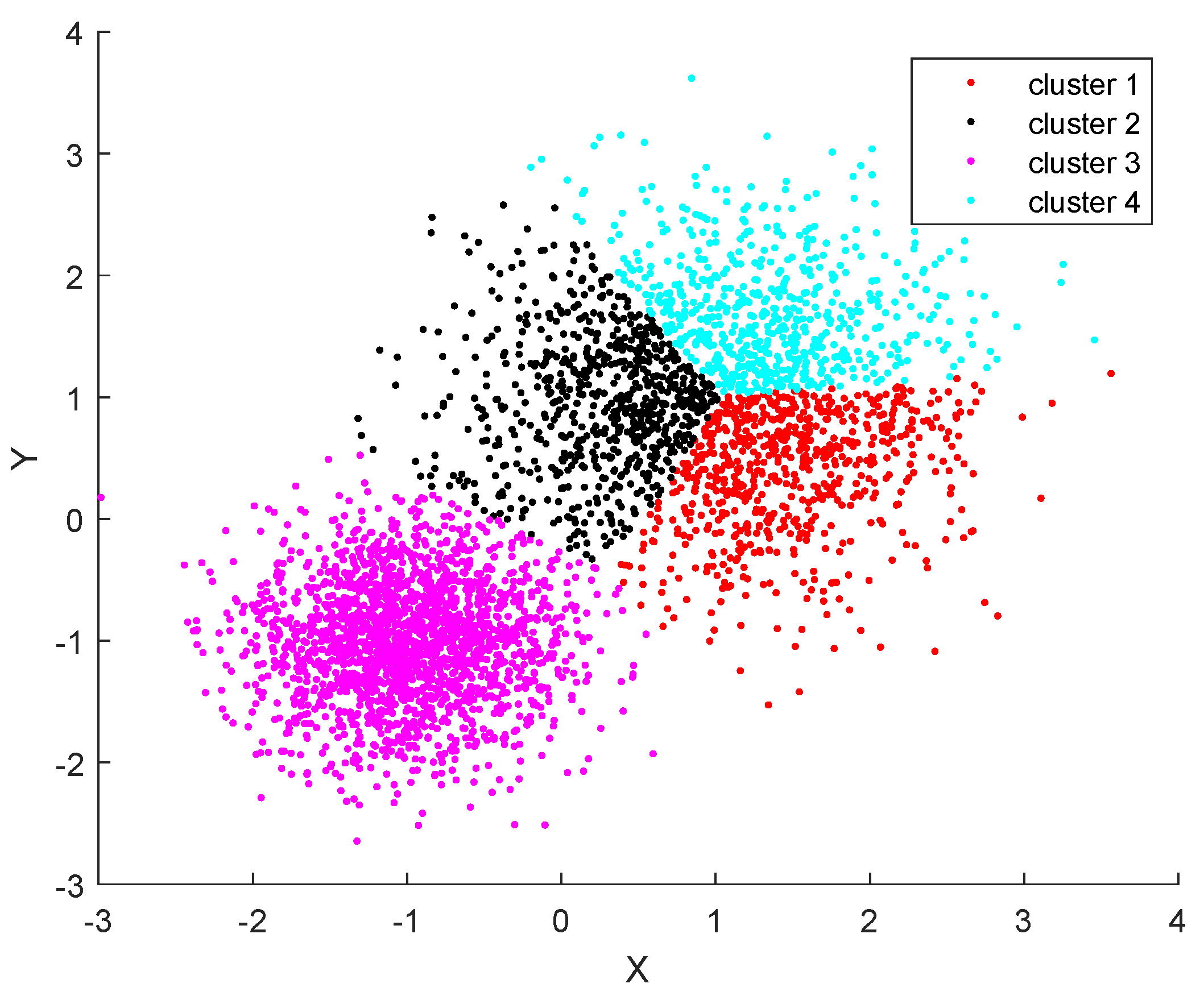
Energies 14 05042 g004
Figure 5. A set of randomly generated samples clustered with the k-means++ algorithm.
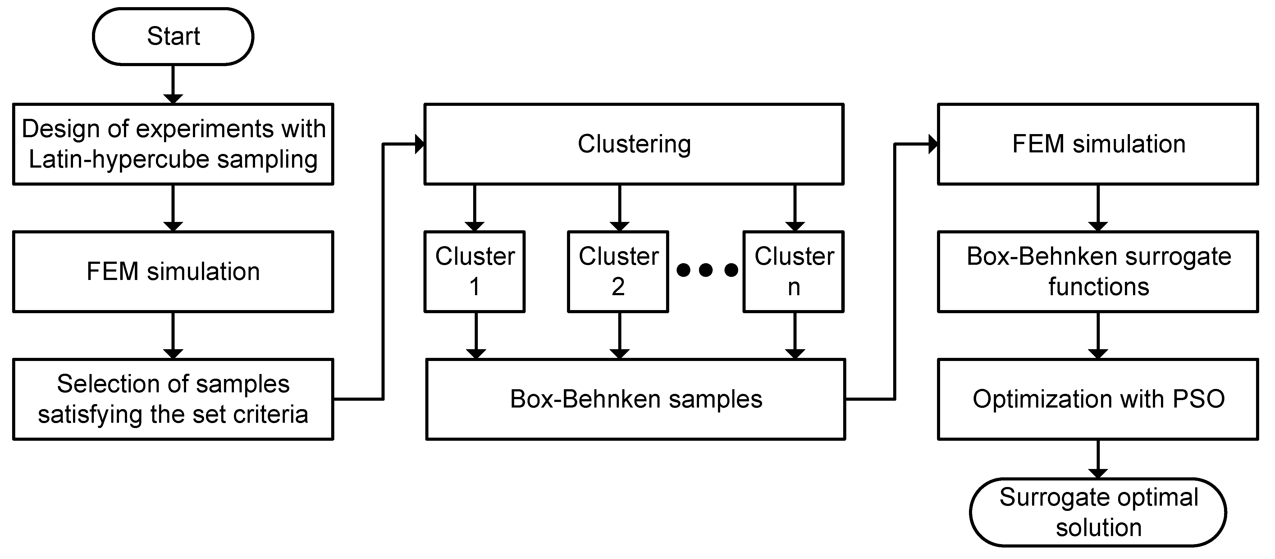
Energies 14 05042 g005
Figure 6. Flow chart: proposed optimization routine—part 1 (surrogate optimization).
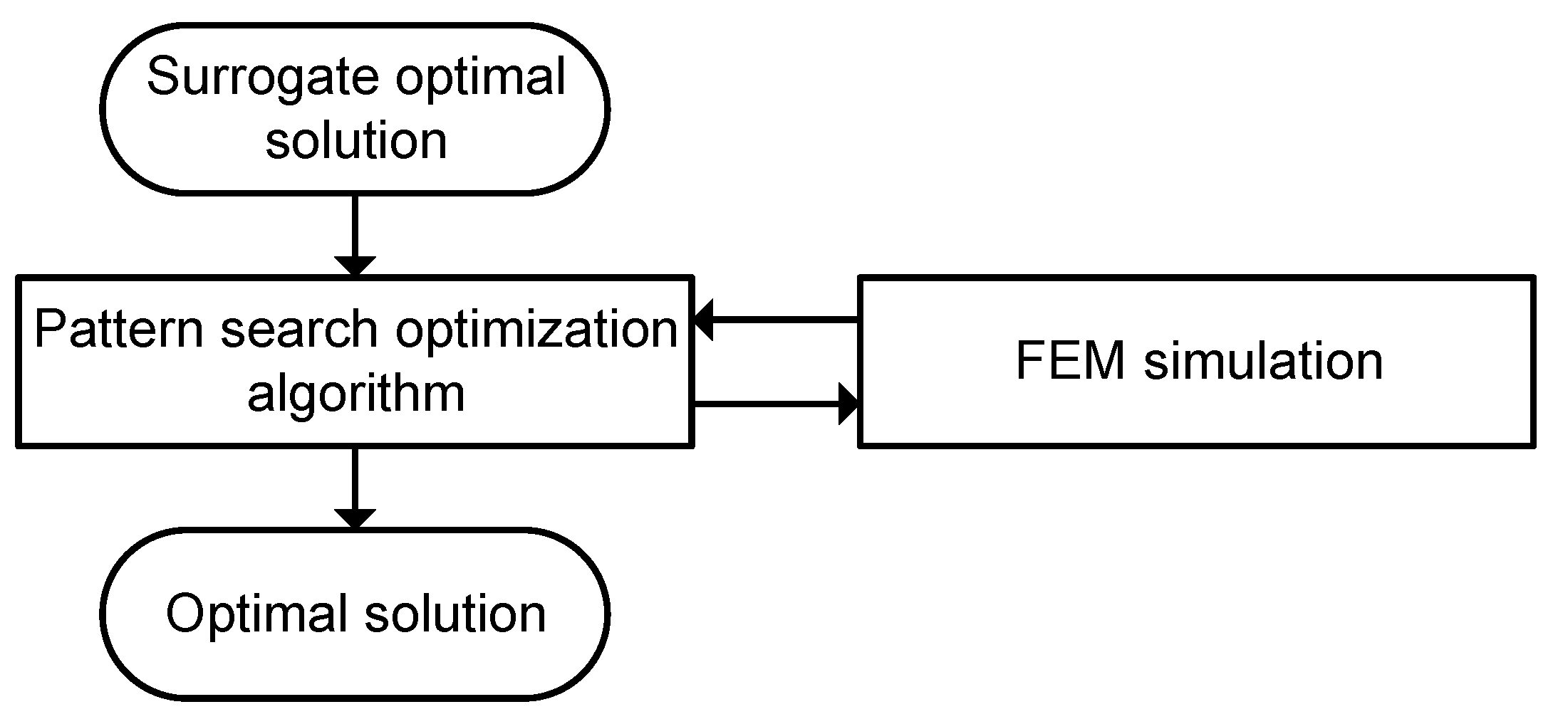
Energies 14 05042 g006
Figure 7. Flow chart: proposed optimization routine—part 2 (pattern search).
Energies 14 05042 g007
Figure 8. Visualization of the process involved in the proposed surrogate optimization routine.
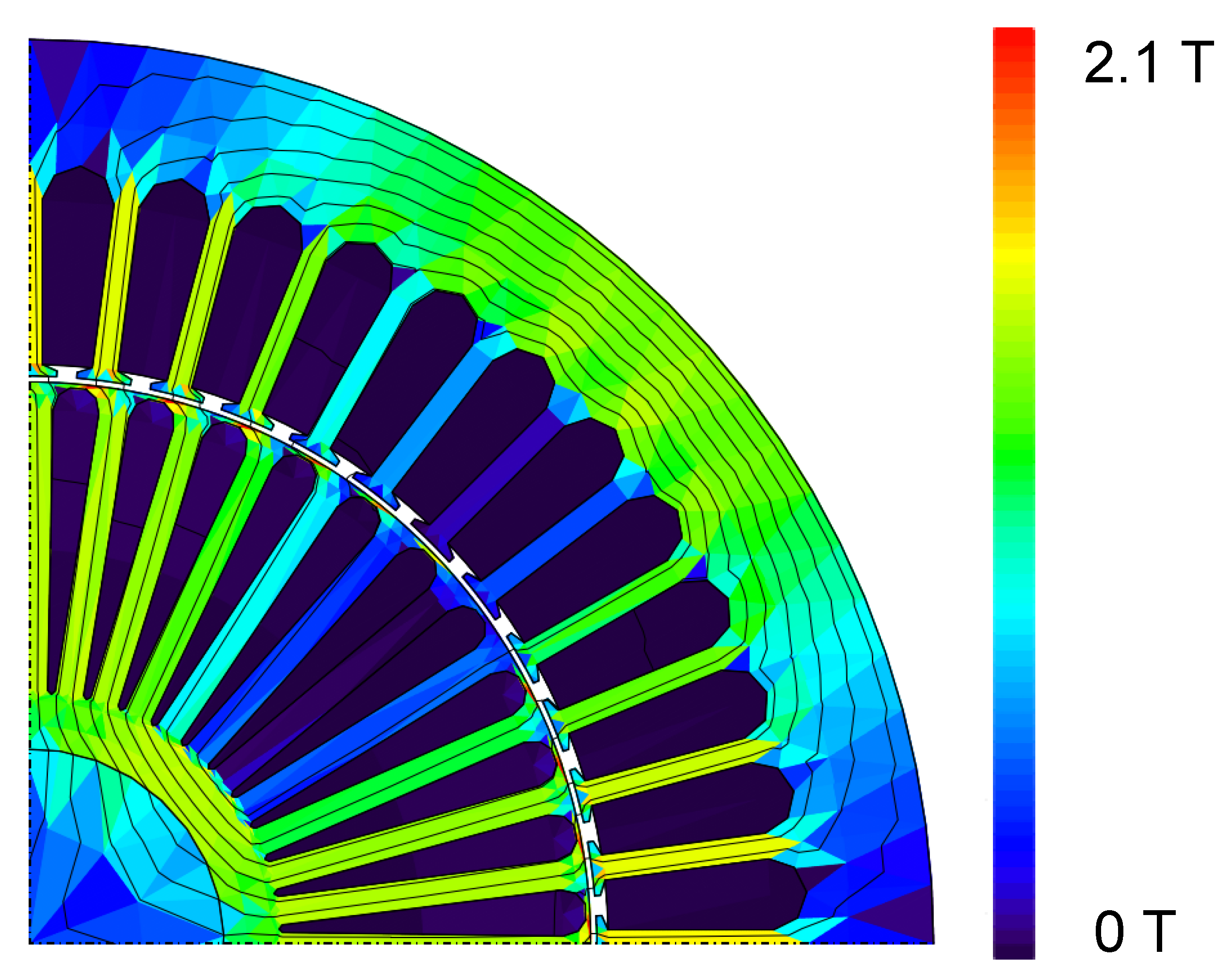
Energies 14 05042 g008
Figure 9. Flux density distribution of the optimal solution from the proposed surrogate optimization routine–multivariate optimization problem.
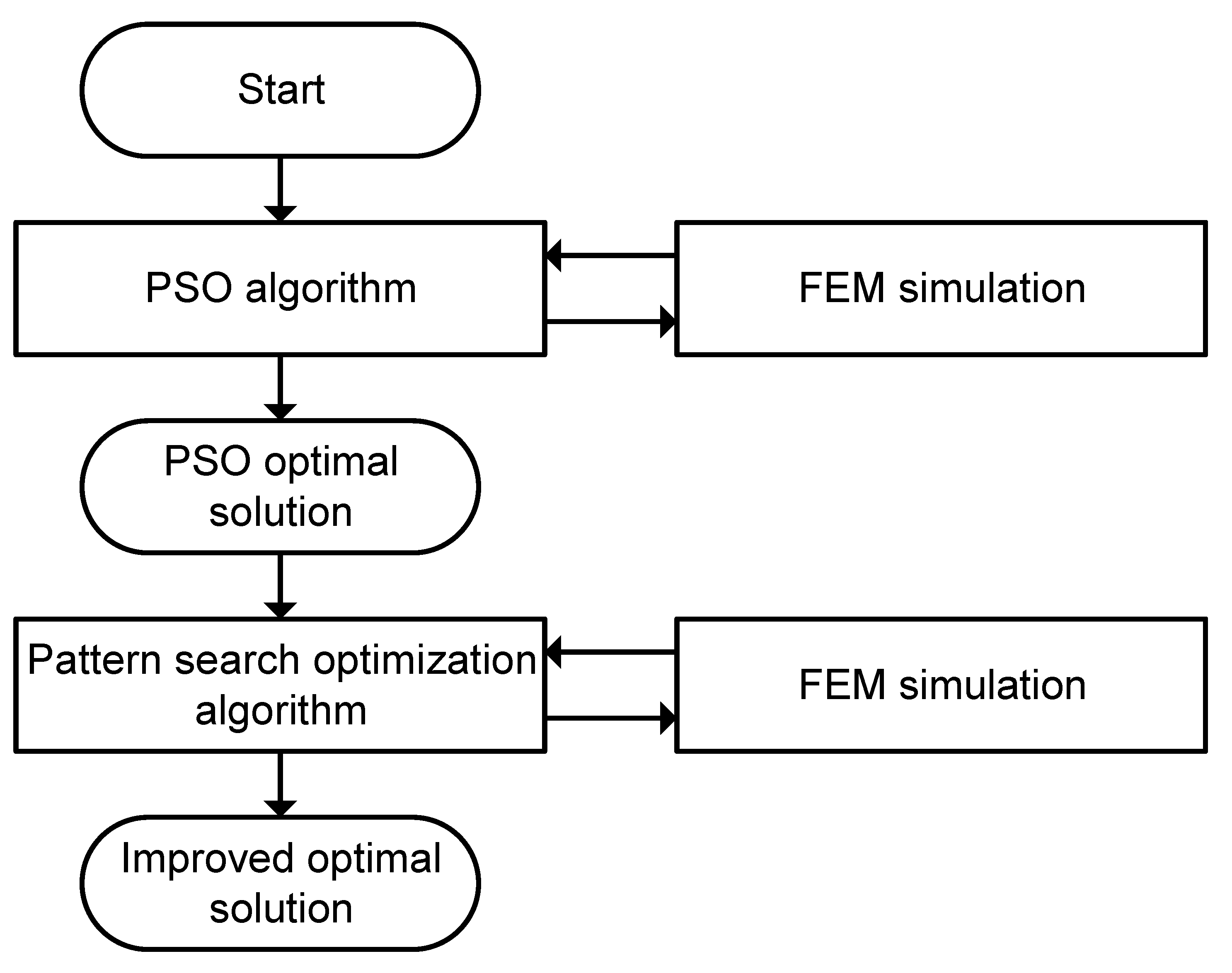
Energies 14 05042 g009
Figure 10. Flow chart: direct optimization routine with FEM as the cost function.
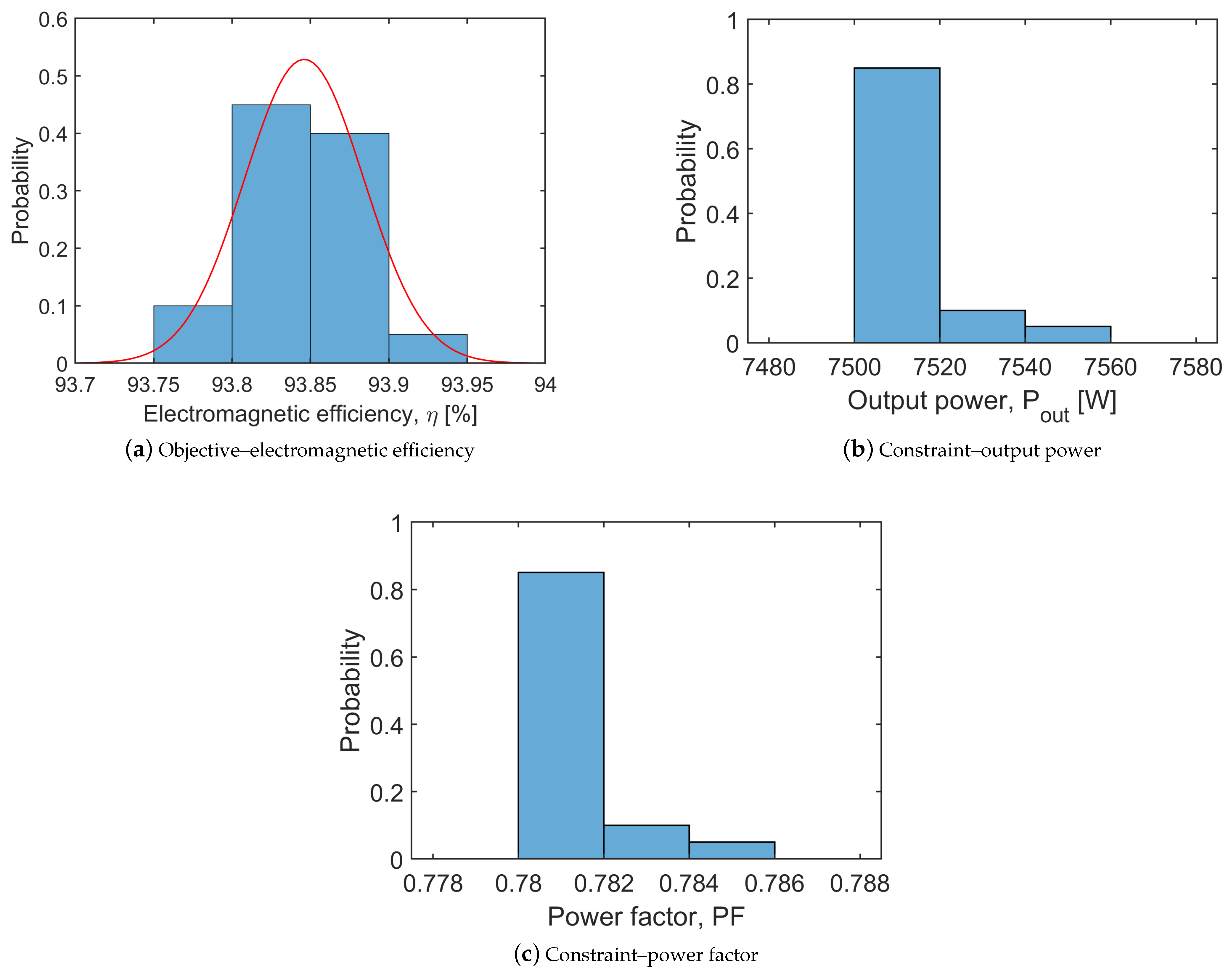
Energies 14 05042 g010
Figure 11. Probability distribution of the objective and constraints from 20 runs of the proposed surrogate optimization routine.
Energies 14 05042 g011
Table 1. Specifications and fixed parameters of the induction motor.
ParameterValue
Output power, P out [W]7500
Line voltage, U l [V]400
Frequency, f [Hz]50
Number of poles, p4
Filling factor-stator slot, K Cu 0.6
Number of conductors-stator slots, Z Qs 28
Number of parallel paths-stator windings, a2
Number of stator slots, N s 48
Number of rotor slots, N r 44
Axial length of the machine, l (mm)220
Stator outer diameter, D se (mm)227.7
Rotor inner (shaft) diameter, D ye (mm)48.98
End-ring overhang length, l oh (mm)40
Conductivity—aluminum (20 °C), σ Al [S/m] 35.5 × 10 6
Conductivity—copper (20 °C), σ Cu [S/m] 57 × 10 6
Table 2. Objective and constraints of the optimization problem.
ObjectiveGoal
Electromagnetic efficiency, η (%)To maximize the electromagnetic efficiency, η
ConstraintsRange
Output power, P out [W]7500 ≤ P out ≤ 7600
Power factor, P F P F ≥ 0.78
Table 3. Optimization variables and their range.
Optimization VariablesRange
Stator inner diameter, D s (mm)120 ≤ D s ≤ 150
Stator tooth width, b ds (mm)2 ≤ b ds ≤ 4
Stator yoke width, h ys (mm)10 ≤ h ys ≤ 30
Slip, s (%)1 ≤ s ≤ 2.1
Air gap width, δ (mm)0.4 ≤ δ ≤ 0.7
Rotor slot upper width, b 4 r (mm)3 ≤ b 4 r ≤ 6
Rotor slot lower width, b 5 r (mm)0.5 ≤ b 5 r ≤ 2
Rotor yoke width, h yr (mm)2 ≤ h yr ≤ 15
Table 4. FEM validation of the optimal solution from Box–Behnken design.
Output ResponseBox–Behnken DesignFEM ValidationDifference
Electromagnetic efficiency, η 95.30%93.31%2.13%
Output power, P o u t 7500.28 W7131.98 W5.18%
Power factor, P F 0.78600.72678.16%
Table 5. Sample selection criteria from the Latin-hypercube sampling method.
Output ResponseSample Selection Criteria
Electromagnetic efficiency, η (%) η ≥ 91
Output power, P out [W]7000 ≤ P out ≤ 8000
Power factor, P F P F ≥ 0.75
Table 6. Validation of surrogate optimal solution of the proposed optimization routine (part 1—surrogate optimization) with FEM simulation 3-variable optimization problem.
Output ResponseSurrogate OptimaFEM ValidationDifference
Electromagnetic efficiency, η 93.63%93.64%0.01%
Output power, P out 7599.97 W7614.76 W0.19%
Power factor, P F 0.78000.78250.32%
Table 7. Surrogate optimal solution compared with the improved optimal solution (part 1—surrogate optimization vs. part 2—pattern search) of the proposed optimization routine 3-variable optimization problem.
Output ResponseOptimal Solution (Part 1)Optimal Solution (Part 2)% Increase
Electromagnetic efficiency, η 93.64%93.66%0.021%
Output power, P out 7614.76 W7572.32 W−0.56%
Power factor, P F 0.78250.7801−0.31%
Table 8. Comparison of design variables of the optimal solution (part 1—surrogate optimization vs. part 2—pattern search) from the proposed surrogate optimization routine 3-variable optimization problem.
Design VariablesOptimal Solution (Part 1)Optimal Solution (Part 2)
Stator inner diameter, D s (mm)147.54146.65
Stator yoke width, h ys (mm)17.0117.27
Slip, s (%)1.121.12
Table 9. Comparison of electromagnetic efficiency and power factor for various load points of the optimal design 3-variable optimization problem.
Output ResponseLoad (100%)Load (75%)Load (50%)
Electromagnetic efficiency, η 93.66%93.74%92.97%
Power factor, P F 0.78010.71220.5888
Table 10. Comparison of losses for various load points of the optimal design 3-variable optimization problem.
LossesLoad (100%)Load (75%)Load (50%)
Stator losses, P stator 335.81 W251.63 W195.66 W
Rotor losses, P rotor 177.18 W124.02 W88.06 W
Total electromagnetic losses, P elec 512.99 W375.65 W283.72 W
Table 11. Validation of surrogate optimal solution of the proposed optimization routine (part 1—surrogate optimization) with FEM simulationdesign–multivariate optimization problem.
Output ResponseSurrogate OptimaFEM ValidationDifference
Electromagnetic efficiency, η 93.48%93.54%0.064%
Output power, P out 7500.16 W7514.74 W0.194%
Power factor, P F 0.79640.79700.075%
Table 12. Surrogate optimal solution compared with the improved optimal solution (part 1—surrogate optimization vs. part 2—pattern search) of the proposed optimization routine–multivariate optimization problem.
Output ResponseOptimal Solution (Part 1)Optimal Solution (Part 2)% Increase
Electromagnetic efficiency, η 93.54%93.90%0.385%
Output power, P out 7514.74 W7502.62 W−0.161%
Power factor, P F 0.79700.7803−2.095%
Table 13. Comparison of design variables of the optimal solution (part 1—surrogate optimization vs. part 2—pattern search) from the the proposed surrogate optimization routine–multivariate optimization problem.
Design VariablesOptimal Solution (Part 1)Optimal Solution (Part 2)
Stator inner diameter, D s (mm)142.77142.77
Stator tooth width, b ds (mm)3.283.30
Stator yoke width, h ys (mm)19.6515.80
Slip, s (%)1.261.26
Air gap width, δ (mm)0.680.70
Rotor slot upper width, b 4 r (mm)5.785.78
Rotor slot lower width, b 5 r (mm)0.880.88
Rotor yoke width, h yr (mm)6.816.81
Table 14. Comparison of electromagnetic efficiency and power factor for various load points of the optimal design–multivariate optimization problem.
Output ResponseLoad (100%)Load (75%)Load (50%)
Electromagnetic efficiency, η 93.90%93.95%93.19%
Power factor, P F 0.78030.71640.5944
Table 15. Comparison of losses for various load points of the optimal design 3-variable optimization problem.
LossesLoad (100%)Load (75%)Load (50%)
Stator losses, P stator 305.44 W234.83 W185.66 W
Rotor losses, P rotor 181.89 W127.15 W88.77 W
Total electromagnetic losses, P elec 487.33 W361.98 W274.43 W
Table 16. Optimal design from the proposed surrogate optimization routine compared with the direct optimization routine.
Output ResponseProposed Surrogate Optimization RoutineDirect Optimization Routine
Electromagnetic efficiency, η 93.90%93.89%
Output power, P out 7502.62 W7505.29 W
Power factor, P F 0.78030.7801
Table 17. Design variables of the optimal solution from the the proposed surrogate optimization routine compared with direct optimization routine.
Design VariablesProposed Surrogate Optimization RoutineDirect Optimization Routine
Stator inner diameter, D s (mm)142.77142.09
Stator tooth width, b ds (mm)3.303.40
Stator yoke width, h ys (mm)15.8015.28
Slip, s (%)1.261.30
Air gap width, δ (mm)0.700.70
Rotor slot upper width, b 4 r (mm)5.785.80
Rotor slot lower width, b 5 r (mm)0.881.34
Rotor yoke width, h yr (mm)6.819.50
Table 18. Comparison of electromagnetic efficiency and power factor for various load points of the optimal design—proposed surrogate optimization routine vs. direct optimization routine.
LoadOutput ResponseProposed Surrogate Optimization RoutineDirect Optimization Routine
100%Electromagnetic efficiency, η 93.90%93.89%
100%Power factor, P F 0.78030.7801
75%Electromagnetic efficiency, η 93.95%93.94%
75%Power factor, P F 0.71640.7159
50%Electromagnetic efficiency, η 93.19%93.16%
50%Power factor, P F 0.59440.5926
Table 19. Comparison of losses for various load points of the optimal design-proposed surrogate optimization routine vs. direct optimization routine.
LoadLossesProposed Surrogate Optimization RoutineDirect Optimization Routine
100%Stator losses, P stator 305.44 W302.42 W
100%Rotor losses, P rotor 181.89 W185.6 W
100%Total electromagnetic losses, P elec 487.33 W488.01 W
75%Stator losses, P stator 234.83 W233.65 W
75%Rotor losses, P rotor 127.15 W129.37 W
75%Total electromagnetic losses, P elec 361.98 W363.03 W
50%Stator losses, P stator 185.66 W185.60 W
50%Rotor losses, P rotor 88.77 W89.78 W
50%Total electromagnetic losses, P elec 274.43 W275.38 W
Table 20. Comparison of the number of FEM simulations in proposed surrogate optimization routine and direct optimization routine.
ParameterProposed Surrogate Optimization RoutineDirect Optimization Routine
Number of FEM simulations136475,208
Publisher’s Note: MDPI stays neutral with regard to jurisdictional claims in published maps and institutional affiliations.

