3.1. Parameters and Occupancy Estimation
The proposed methodology has been implemented to estimate the parameters
, as well as the occupancy vector for a set of given data, that stem from the EM solution of the stochastic differential Equation (
5). All mentioned algorithms have been programmed in MATLAB.
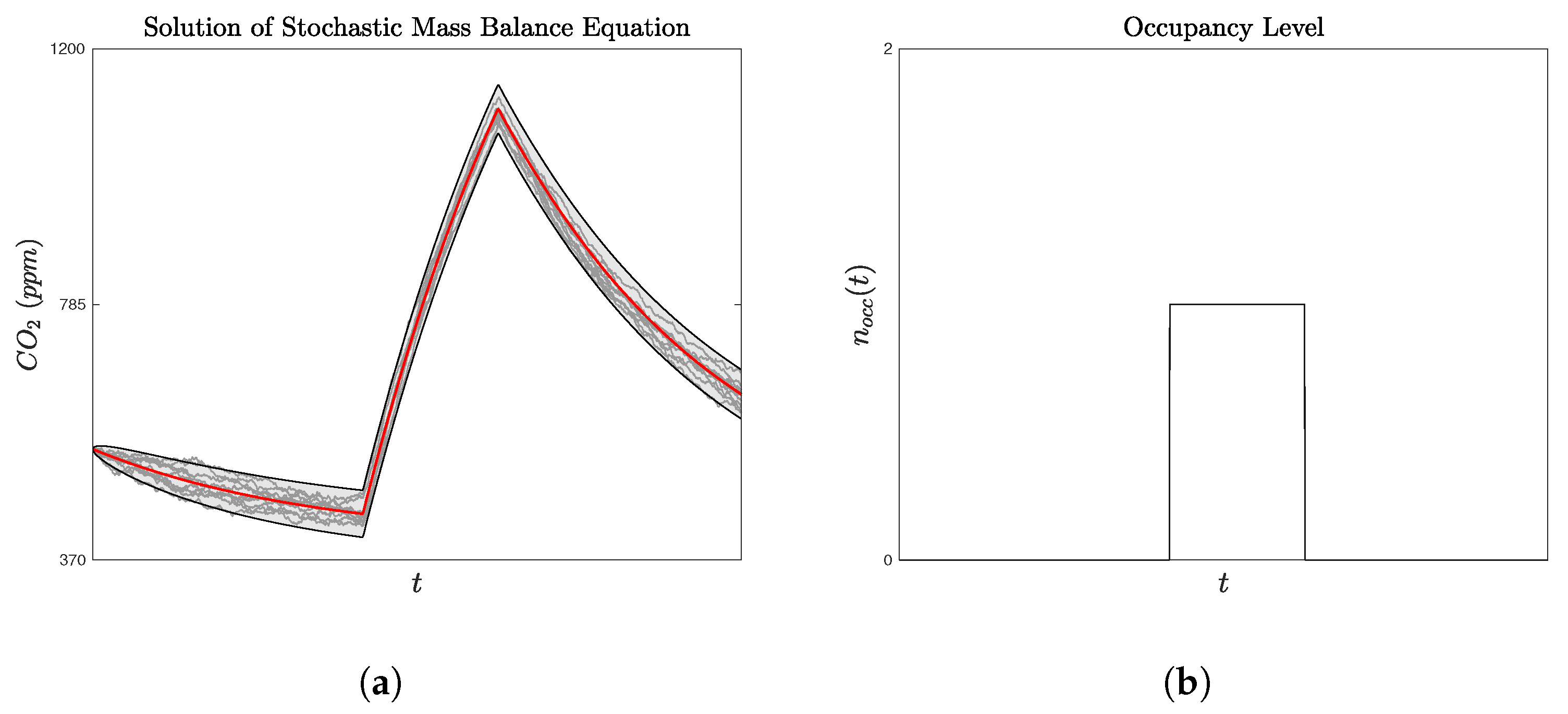
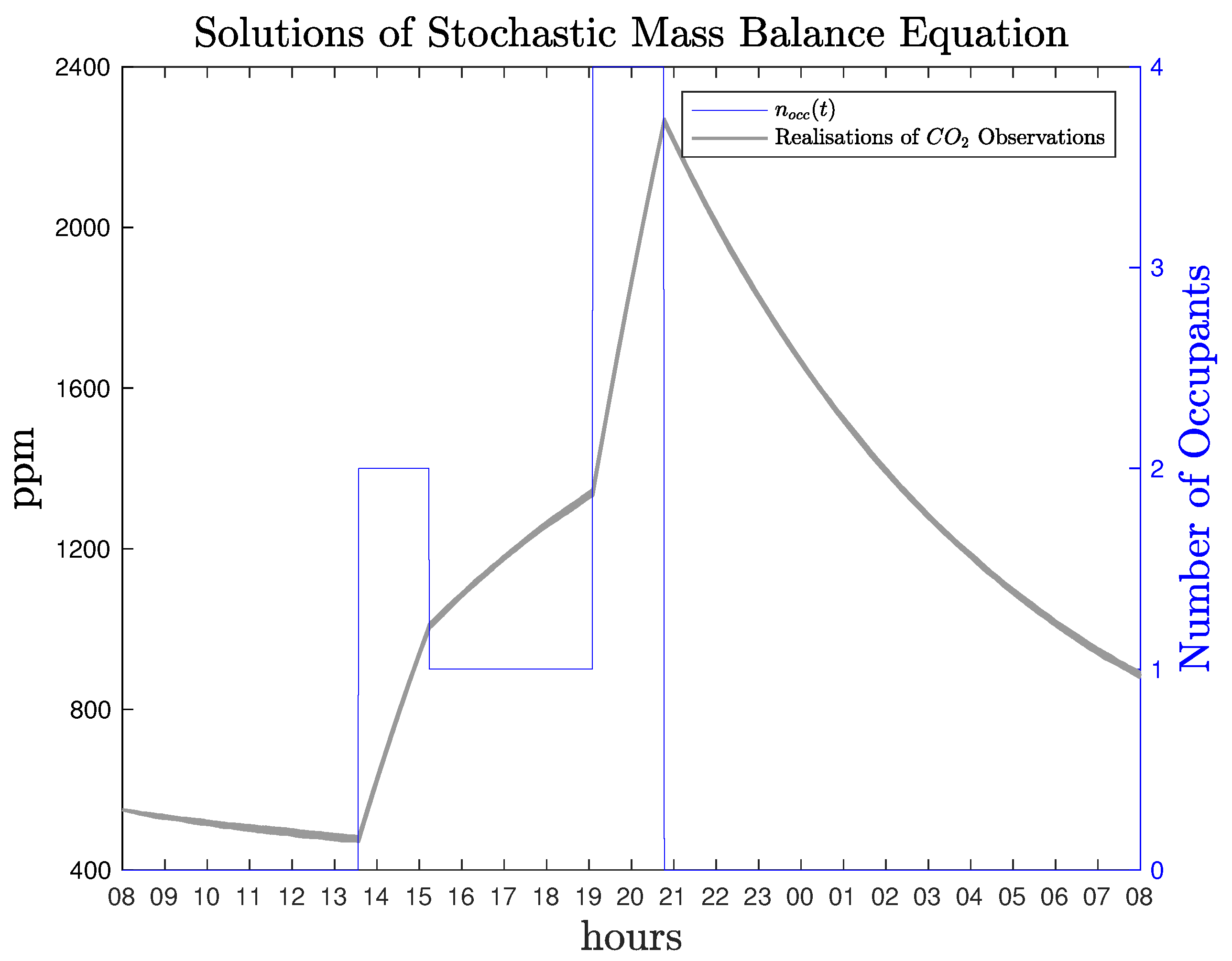
Figure 5 illustrates ten solution paths of the stochastic differential equation, where the parameters are chosen as:
[
36],
(ppm) [
10],
(ppm/h), [
14], and
[
14]. A profile
materialises a simple scenario of presence in a room.
In order to replicate a realistic problem, a single realisation of the solution is considered, and the time series is used to estimate the parameters using the method of evolutionary maximisation of the likelihood function. In the last figure, it is clear that the solution of the stochastic mass balance equation reflects the fact that when occupants are present in the room, e.g., approximately at 13:40 to almost 21:00, the CO2 increases as expected. When vanishes, then the solution has a mean reverting behaviour (Ornstein–Uhlenbeck Process.), analogous to the infiltration rate.
The estimation algorithm has been implemented using a maximum number of generations
, a population of
, a crossover probability
and a mutation scaling
F sampled uniformly from
. The estimated parameters of the proposed method are given in
Table 1.
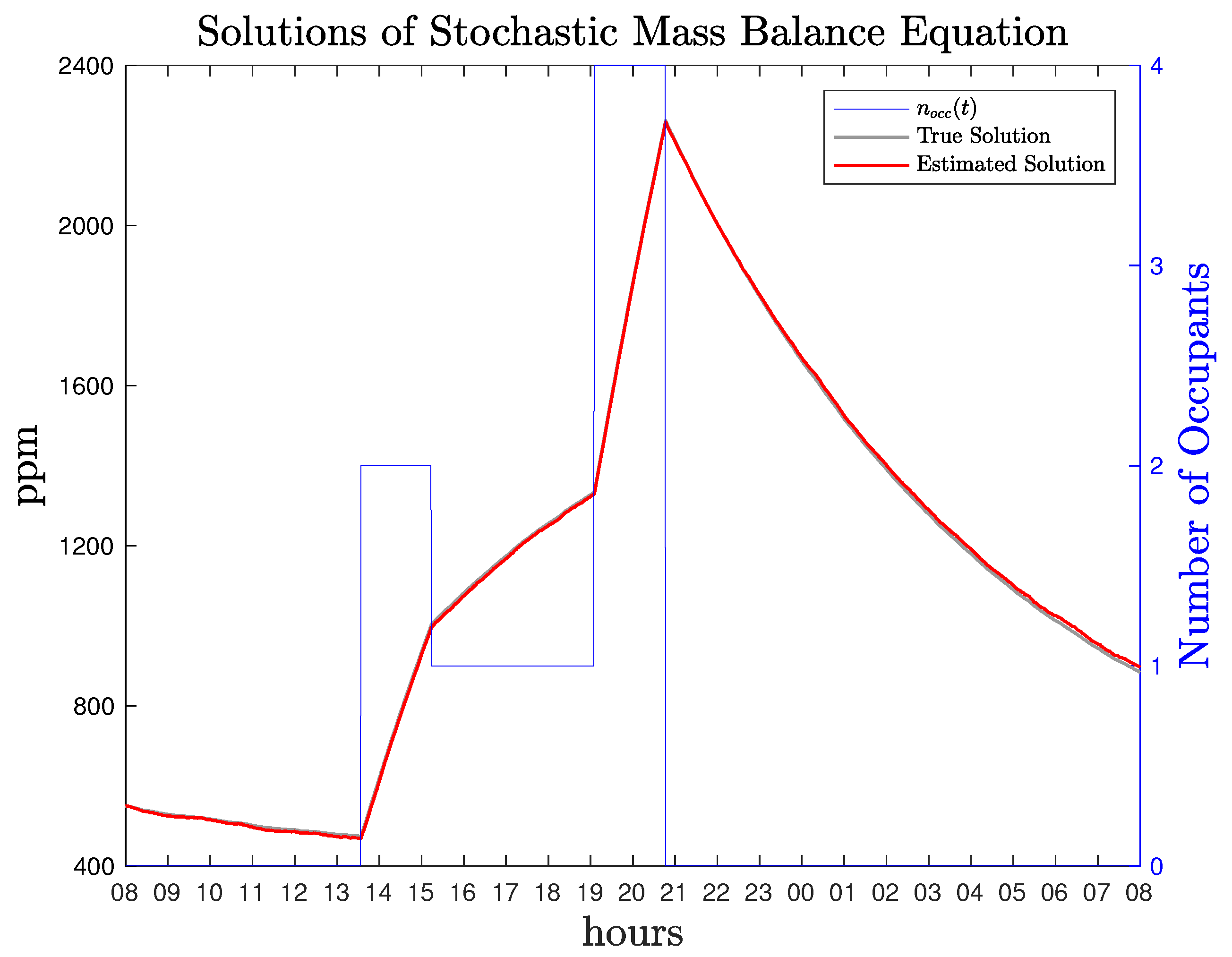
Figure 6, illustrates the solution of the stochastic model, i.e., the training data, and the model’s solution corresponding to the estimated parameters. The solution of the differential equation using the estimated parameters
is in very close vicinity to the true solution.
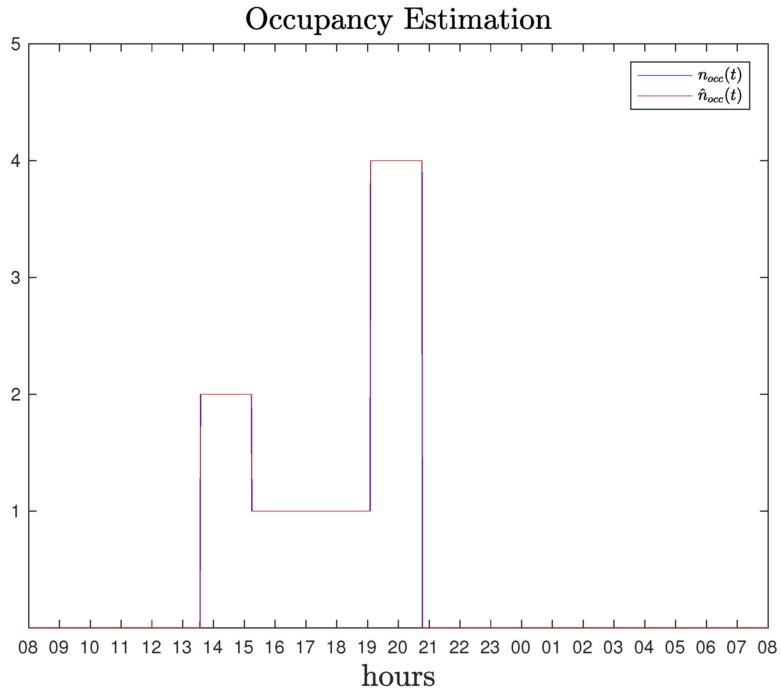
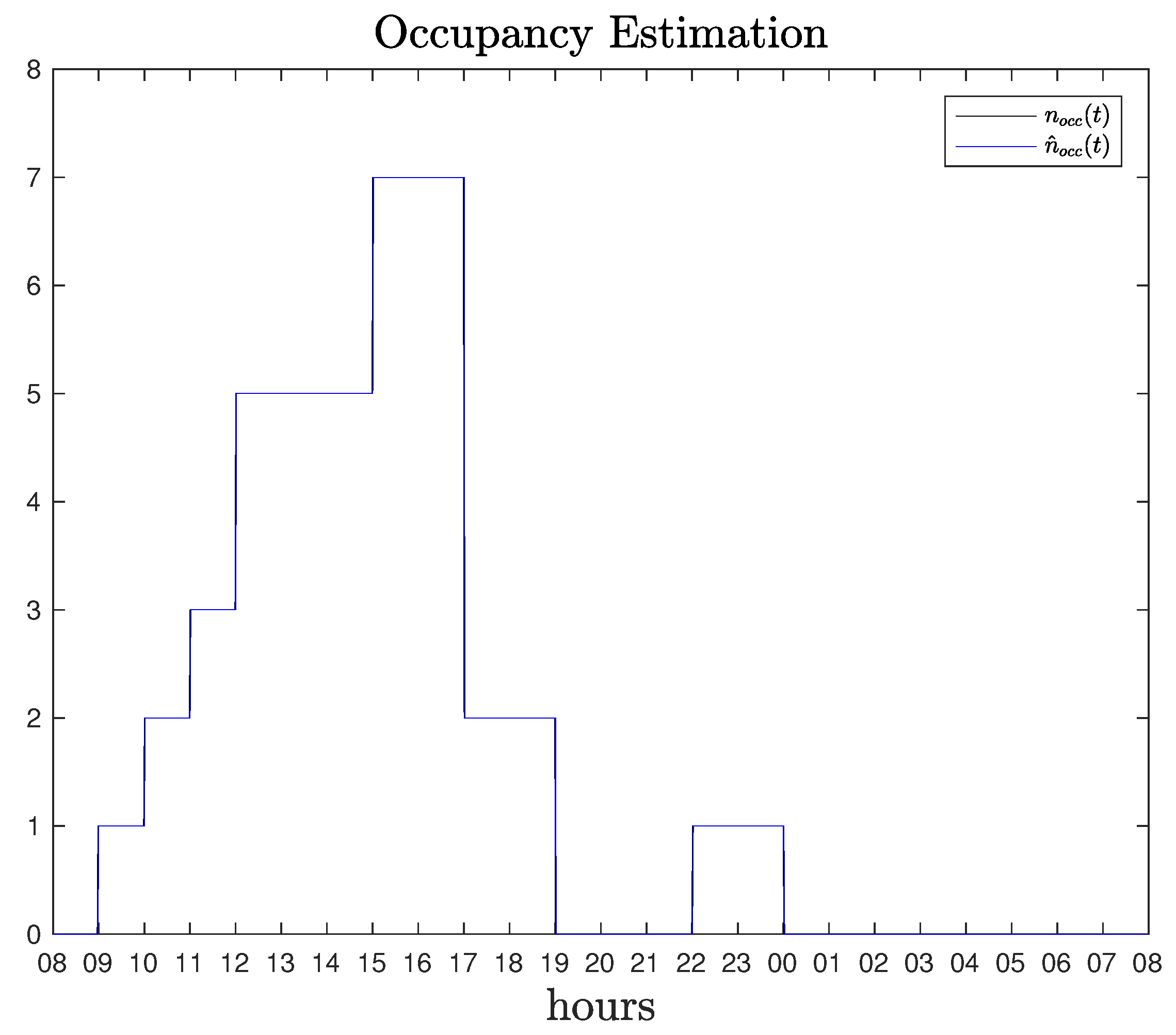
The occupancy estimation algorithm, has been implemented in the latter case and the estimation
is identical to the ground truth,
. The result is illustrated in
Figure 7.
The performance of both the parameter estimation method, as well as the occupancy estimation algorithm is excellent. For the implementation of the occupancy algorithm, 1440 points of CO2 concentration are used, after having generated them from the numerical solution of the mass balance equation; using the method of Euler–Maruyama. Furthermore, the estimated parameter has been used, as described in the section of occupancy estimation algorithm. The number of iterations for the algorithm has been set to 1000.
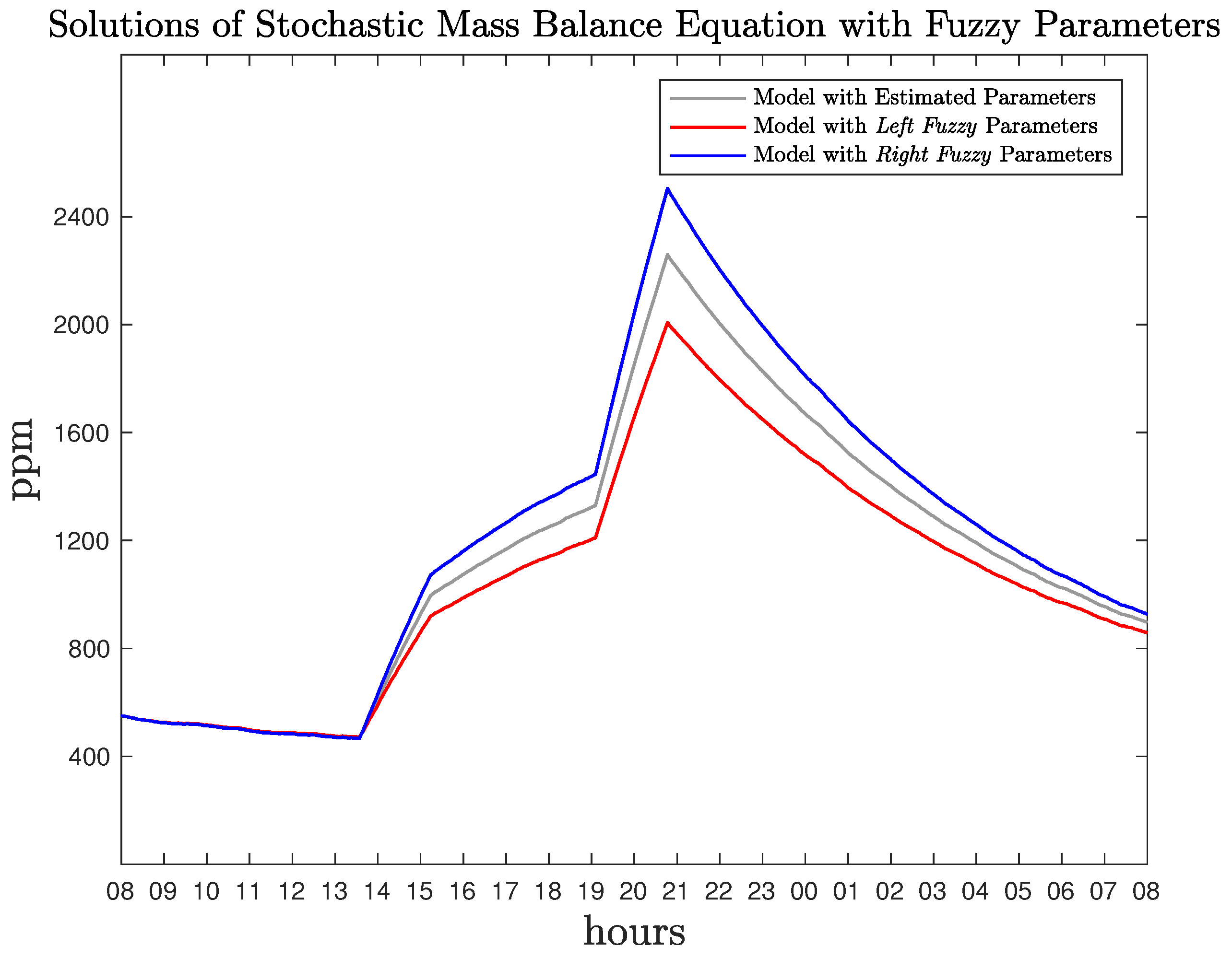
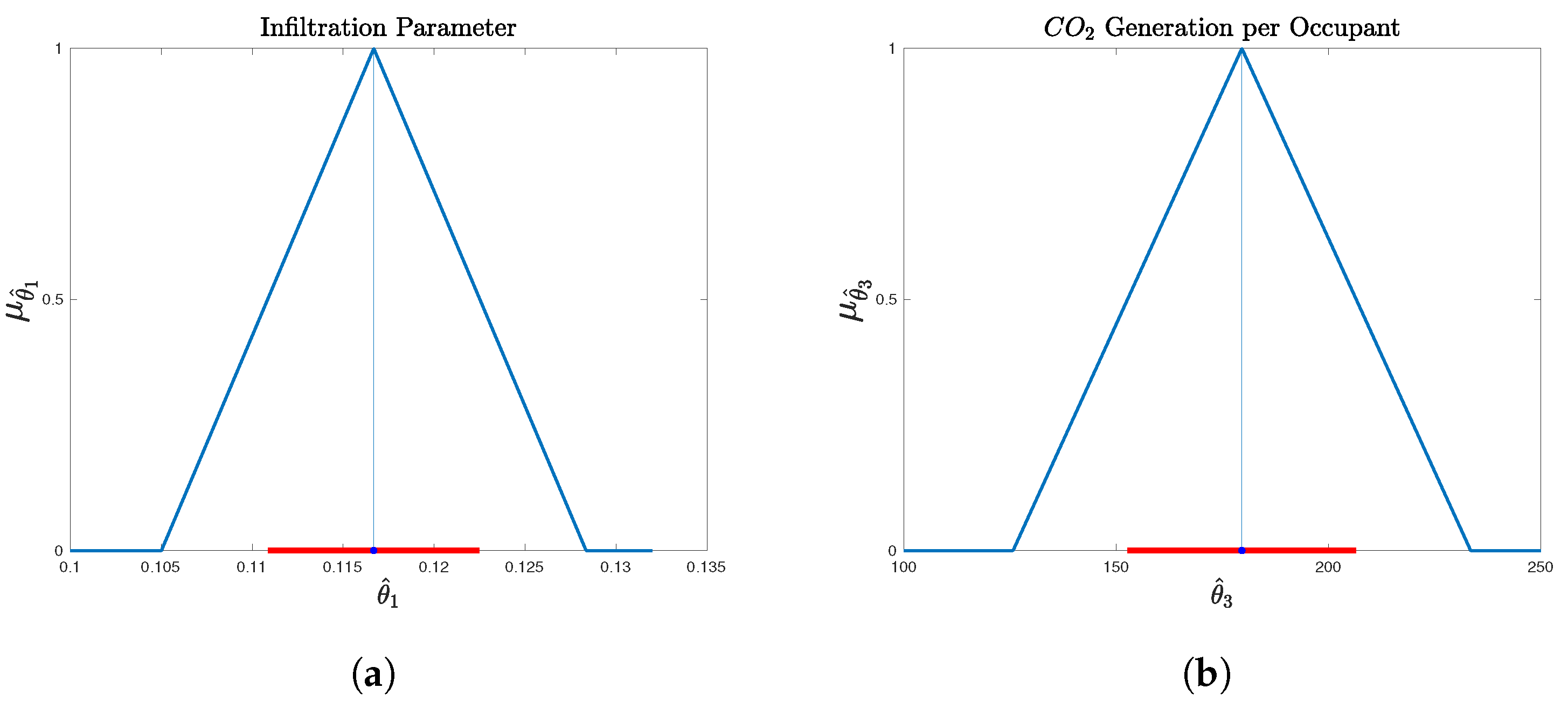
To study the result of parametric uncertainty on the occupancy estimation algorithm, the estimated infiltration rate and the estimated CO
2 generation per occupant, are modelled using fuzzy numbers. The parameters of the fuzzy case are computed using the
a-cut method, as previously described, and are illustrated in
Figure 3. The stochastic differential equation solutions using the estimated parameters, as well as the fuzzy estimated parameters (
Table 2) are illustrated in
Figure 8. It is clear that a parametric uncertainty bound is introduced in the model, since fuzzy parameters are considered.
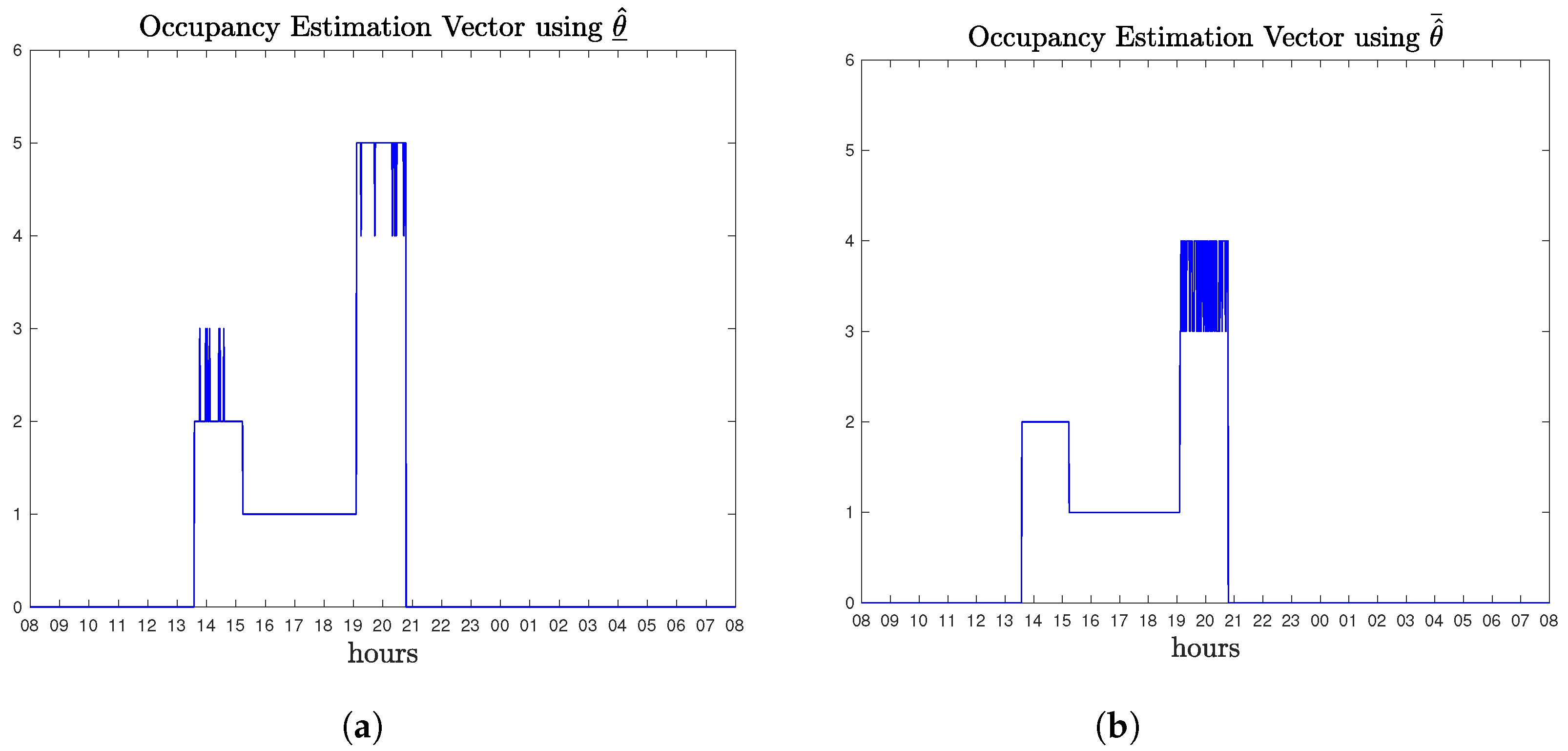
The occupancy estimation algorithm is implemented in the case of both
and
parameters. The results are depicted in
Figure 9. The estimation result produced by the algorithm differs from the real number of occupants, that generate the CO
2 data. By considering the infiltration and the carbon dioxide generation by the occupants as fuzzy, a further uncertainty in the model other than the noise, is induced. The occupancy vector in the case of
is, in some time points, overestimated. This reflects the fact that since CO
2 generation is much lower than the estimated value, then the algorithm, based on the maximum likelihood principle, tries to determine what
should be in order for the training data to be generated. Therefore, it computes an estimation vector
, so that the solution, if considered parameters
, would match the true data. In the case of
the estimated occupancy vector is, in some time points, underestimated reflecting the fact that in some time points the number of occupants should be smaller than 4, in order for the true data to be produced.
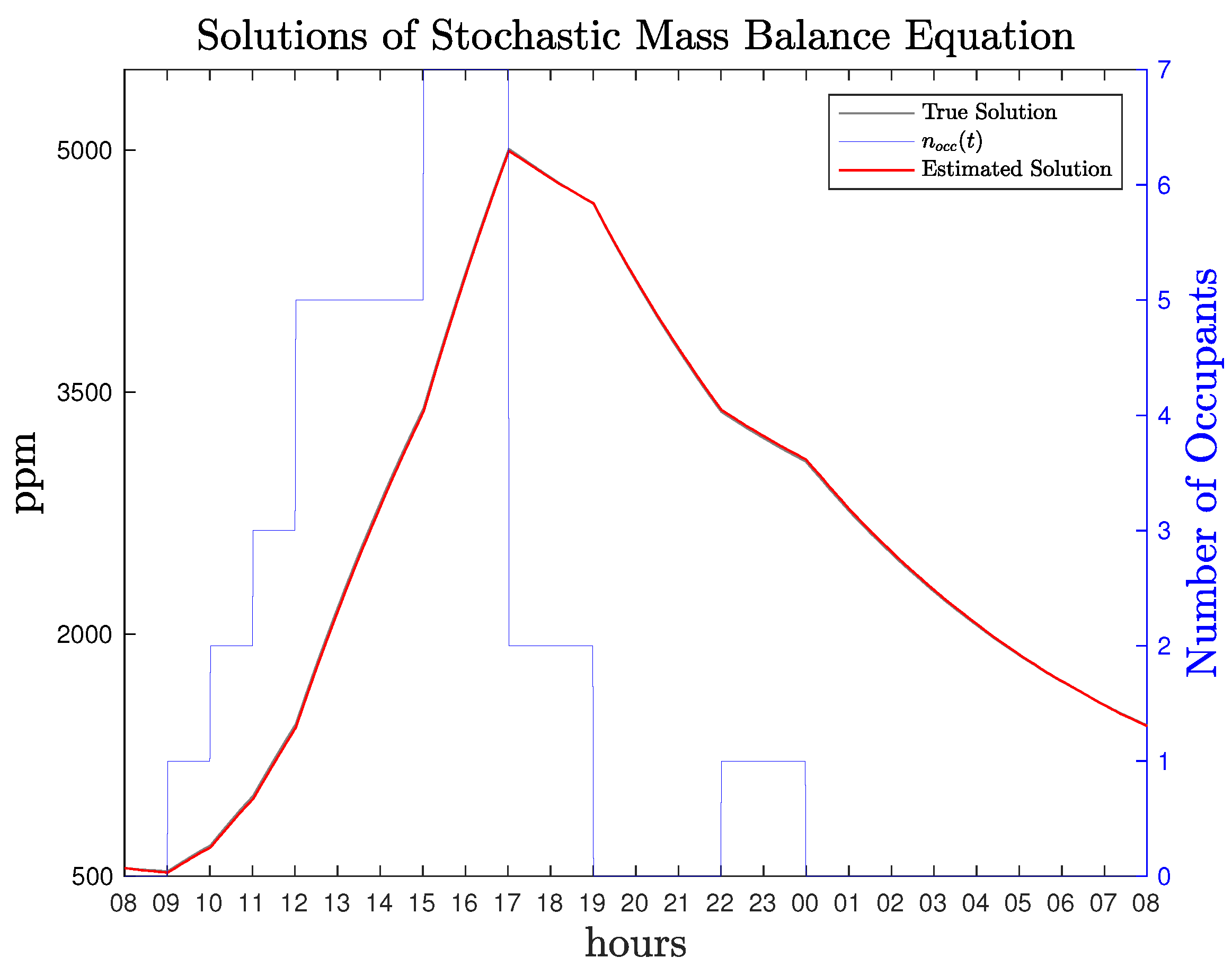
For the MACS development, the proposed methodology is used, for the estimation of an occupancy profile that resembles a working office: an increasing number of occupants are present in the room’s interior until late afternoon. Following to that, a single occupant is present for two hours, until midnight. The occupancy profile and the associated CO
2 concentration, are illustrated in
Figure 10.
The true parameters used in the simulation, as well as their estimation, using differential evolution, are given in
Table 3.
The algorithm of occupancy estimation, performs very accurately and the true occupant vector
is identical to the estimated,
. The results are given in
Figure 11.
Similarly to the previous case, the parametric uncertainty on the parameters is addressed, by assuming that the infiltration and the CO
2 generation per occupant are modelled by triangular fuzzy numbers, with core given by
for
and
for
. Applying the
a-cut methodology the
left and
right parameters were computed to be (
Table 4).
The application of the occupancy algorithm in the case of fuzzy parameters is shown in
Figure 12. The analysis follows the same philosophy as previously described. It is quite interesting, that fuzzy parameters increase the uncertainty in the model, and the occupancy estimation algorithm results in overestimated or underestimated vectors. However, it should be clearly stated that this is not a weak point of the algorithm, but a direct result from the maximum likelihood nature of it.
3.2. Multi Agent Control Framework
As far as the MACS is concerned, the simulation time has been set to one year with a simulation step time of 0.001 h. The data, regarding the ambient temperature, the horizontal diffused illuminance, and the solar irradiance are acquired from the database of the Institute for Environmental Research and Sustainable Development (IERSD), National Observatory of Athens, and they are associated with the year 2019, for Athens, Greece with a sample time of 1 h. For the outdoor CO2 concentration, the constant value of 359.4813 ppm that has been estimated, is used. The set point for the heating/cooling system has been set to 23 °C, when the outdoor temperature falls under 21 °C, and 26 °C when the outdoor temperature exceeds 29 °C. The set point for the indoor illuminance has been set to 700 and the set point for the CO2 concentration has been set to 380 ppm.
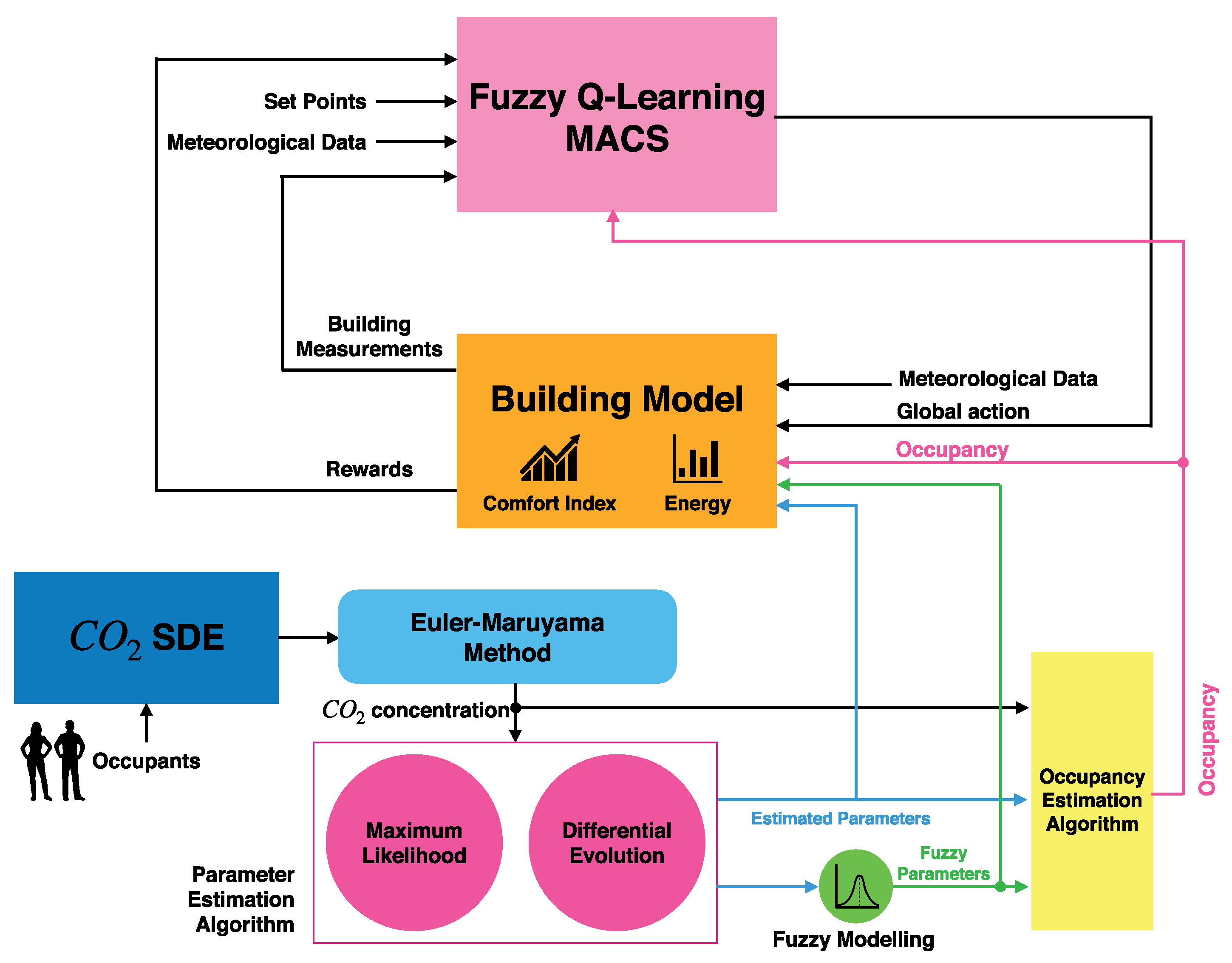
All the sub-models lighting, thermal, CO2 concentration models and the algorithms of the MACS have been implemented in MATLAB/Simulink, each sub-model and each agent is an embedded MATLAB function with multiple inputs and outputs. The relation between inputs and outputs are described by the corresponding algorithms and equations. For example, the CO2 concentration sub-model is a two input (number of occupants and ventilation rate) and one output system (CO2 concentration).
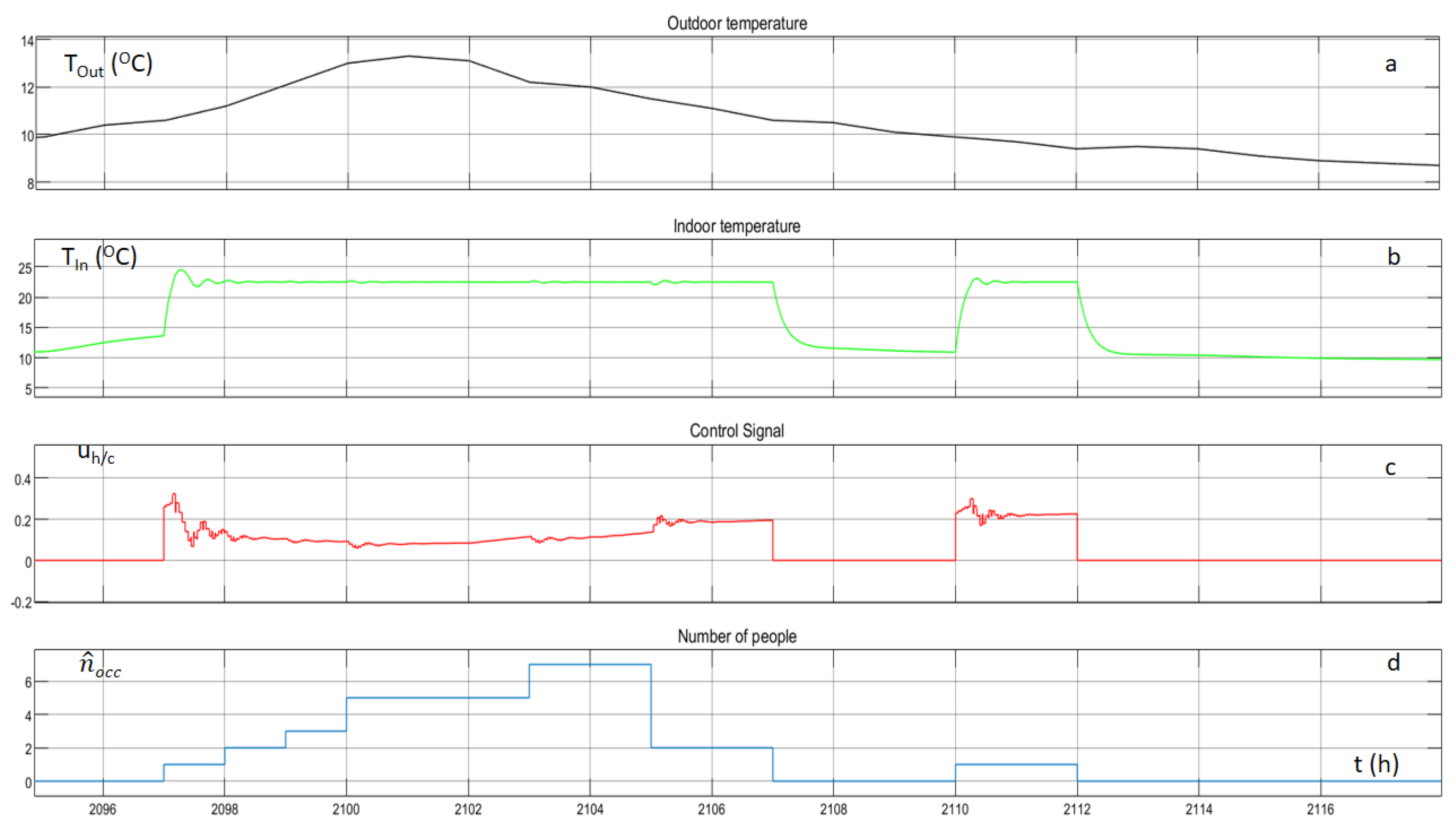
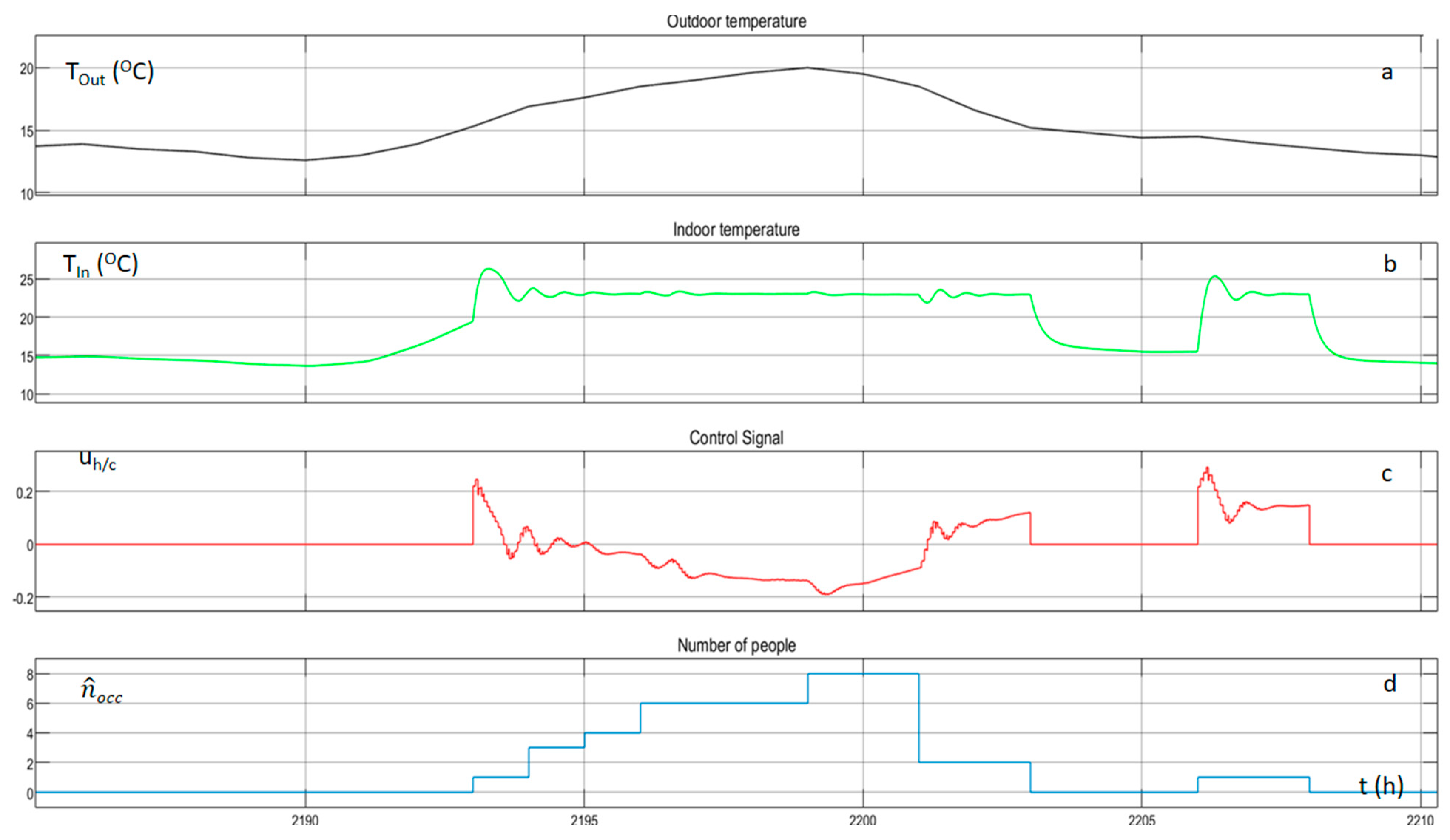
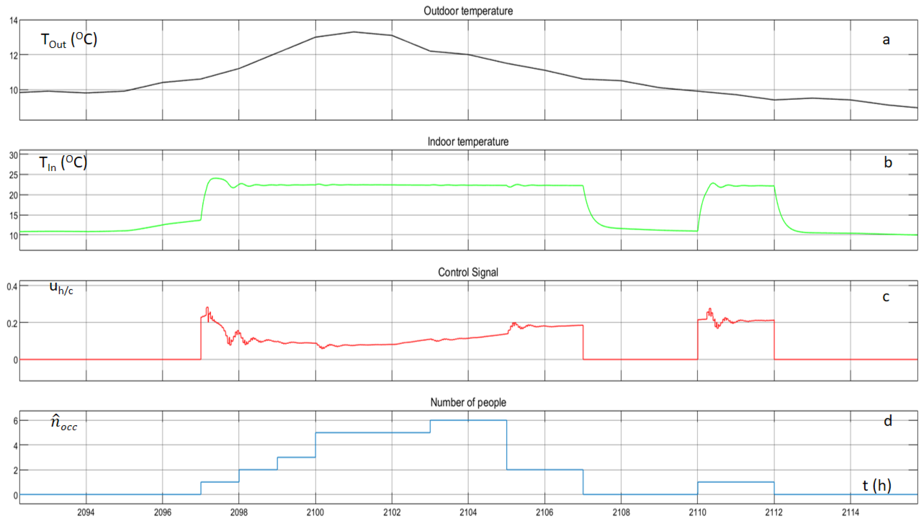
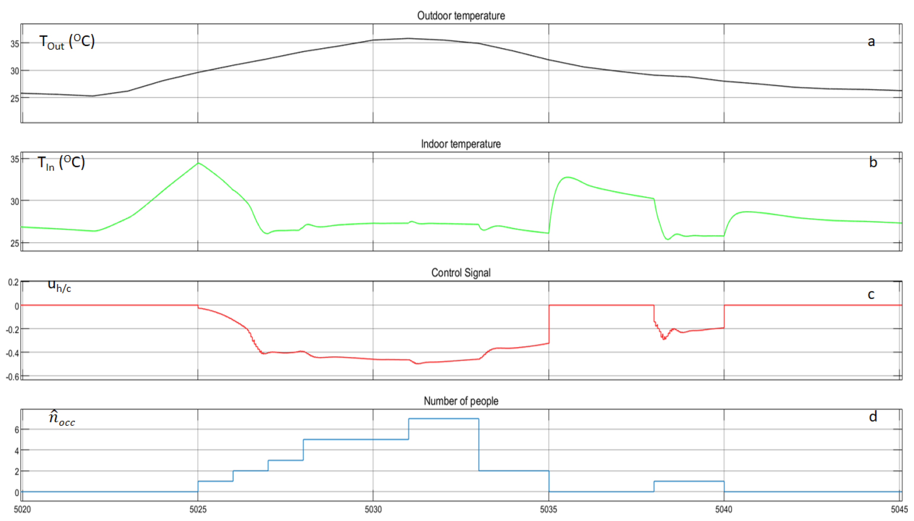
The following figures illustrate the outdoor temperature, the indoor temperature, the control signal of the heating/cooling system and the occupancy of the building. After the extensive exploration, the indoor temperature remains almost constant at 23 °C for the winter and at 26 °C for the summer, during the hours when occupants are present inside the building.
Figure 13 and
Figure 14 are associated with one random day of winter and one random day of summer, respectively. When the occupancy level of the building is zero, the control signal of the agent is zero and consequently the indoor temperature is lower from the set point for the winter and above the set point for the summer. When occupants are entering the building the agent starts to operate again and the indoor temperature is reaching the set point with small oscillations.
A similar philosophy follows
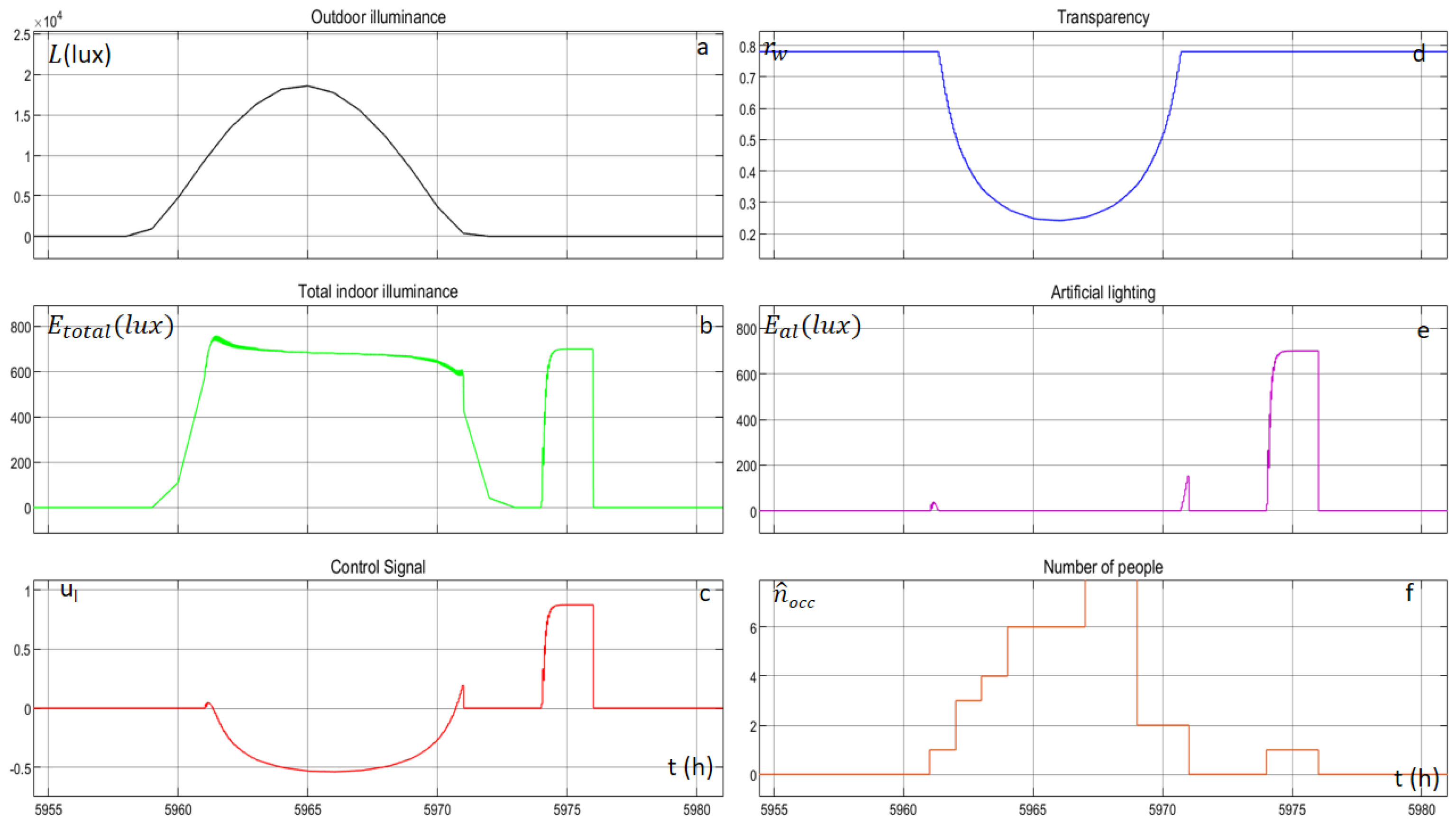
. At first, the corresponding agent visits new states and mainly explores the state-action space. Following the exploration, the indoor illuminance remains almost constant at 700
, at the hours of existing occupancy.
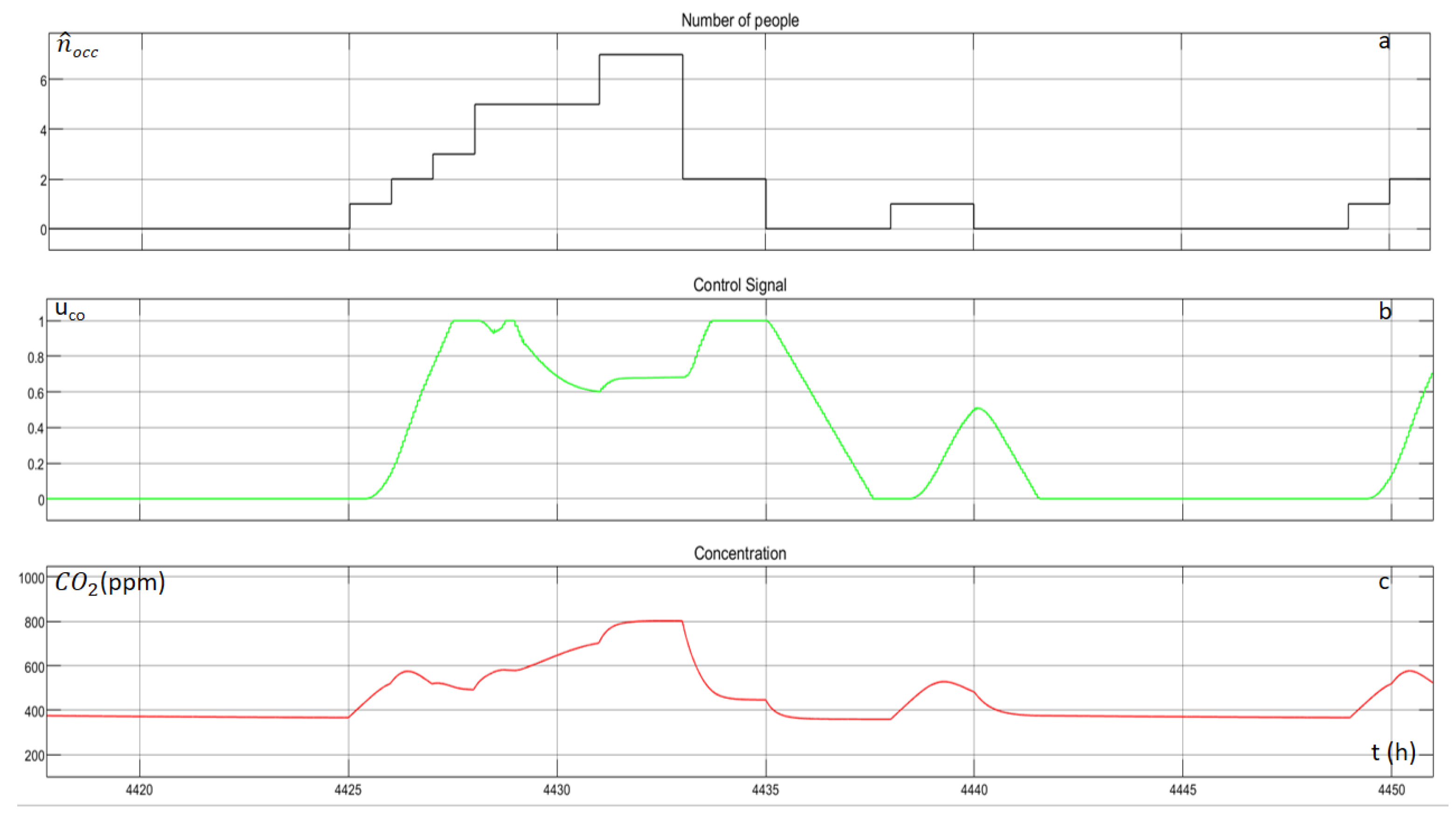
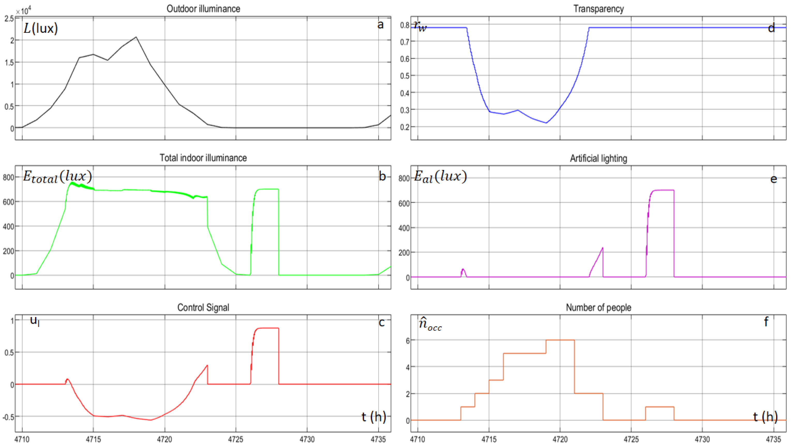
Figure 15 depicts the outdoor horizontal diffused illuminance, the total indoor illuminance, the control signal, the transparency of the electro-chromic window, the provided illuminance by the artificial lighting system and the number of people inside the building, for a random day. When the occupancy of the building is zero, the control signal of the agent is zero, and consequently the indoor illuminance is proportional to the outdoor horizontal illuminance. When occupants enter the building, the agent starts to operate again and the indoor horizontal illuminance is reaching the set point with small oscillations, by either changing the transparency of the window or by changing the illuminance of the artificial lighting.
Figure 16 illustrate the occupancy of the building, the control signal of the agent and the indoor CO
2 concentration, for one random day. The agent explores in the beginning and after the exploration, the indoor concentration of the CO
2 remains lower than the value of 800 ppm. The ventilation system operates when there are people inside the building, and either reduces or stop its operation, when the occupancy level vanishes, and consequently the concentration of the CO
2 is reduced.
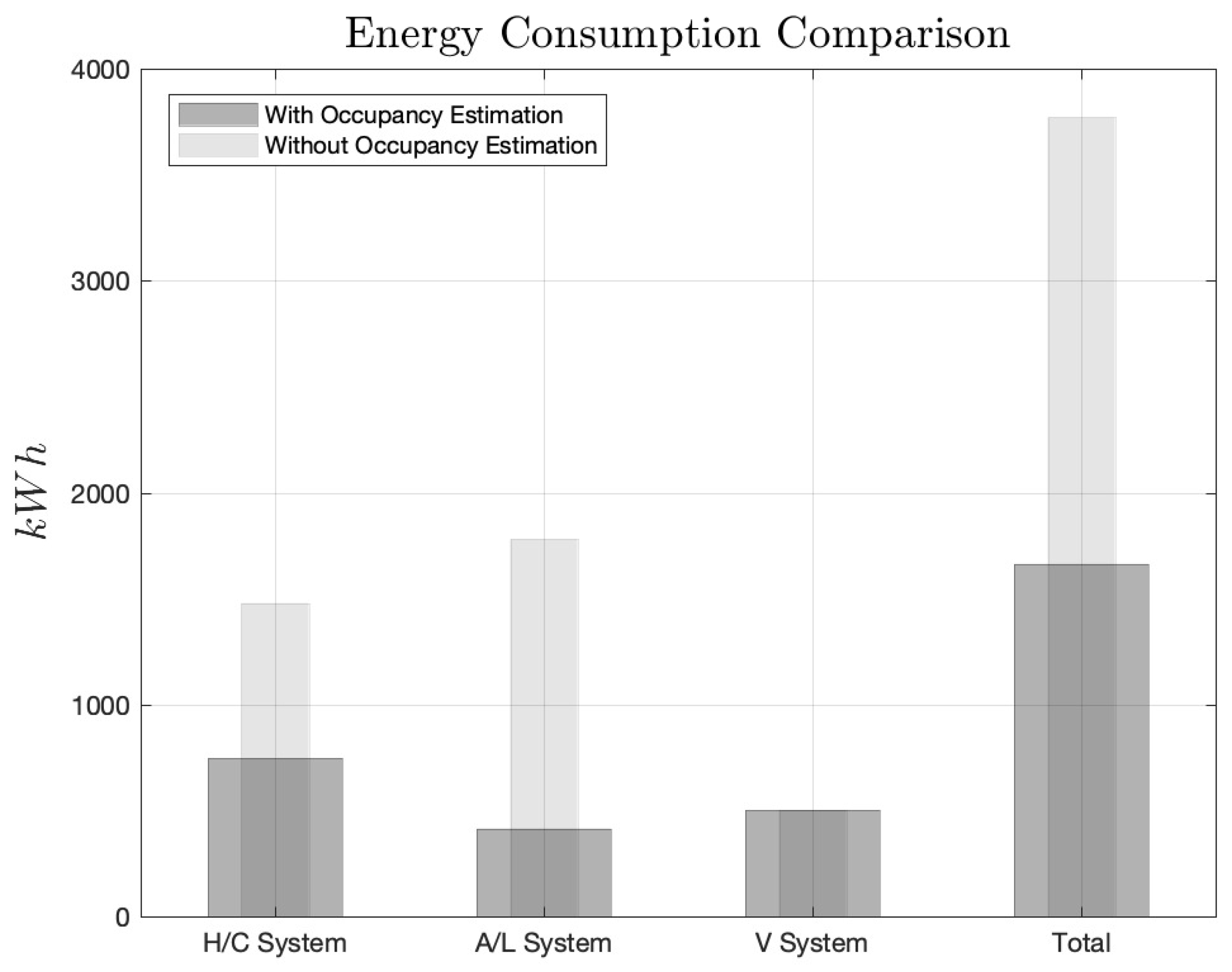
The overall energy consumption of the three systems: heating/cooling (H/C) system, artificial lighting (A/L) system and ventilation (V) system for one year period is computed as 1663 kWh in relation to the much larger value 3770 kWh, which is the overall consumption of these systems for the same year without taking into account the occupancy of the building: the heating/cooling system, as well as the lighting system, operate only for hours where . This concludes an overall reduction of .
The consumptions of each system, with and without regarding the occupancy of the building, are presented in
Table 5 and graphically illustrated in
Figure 17.
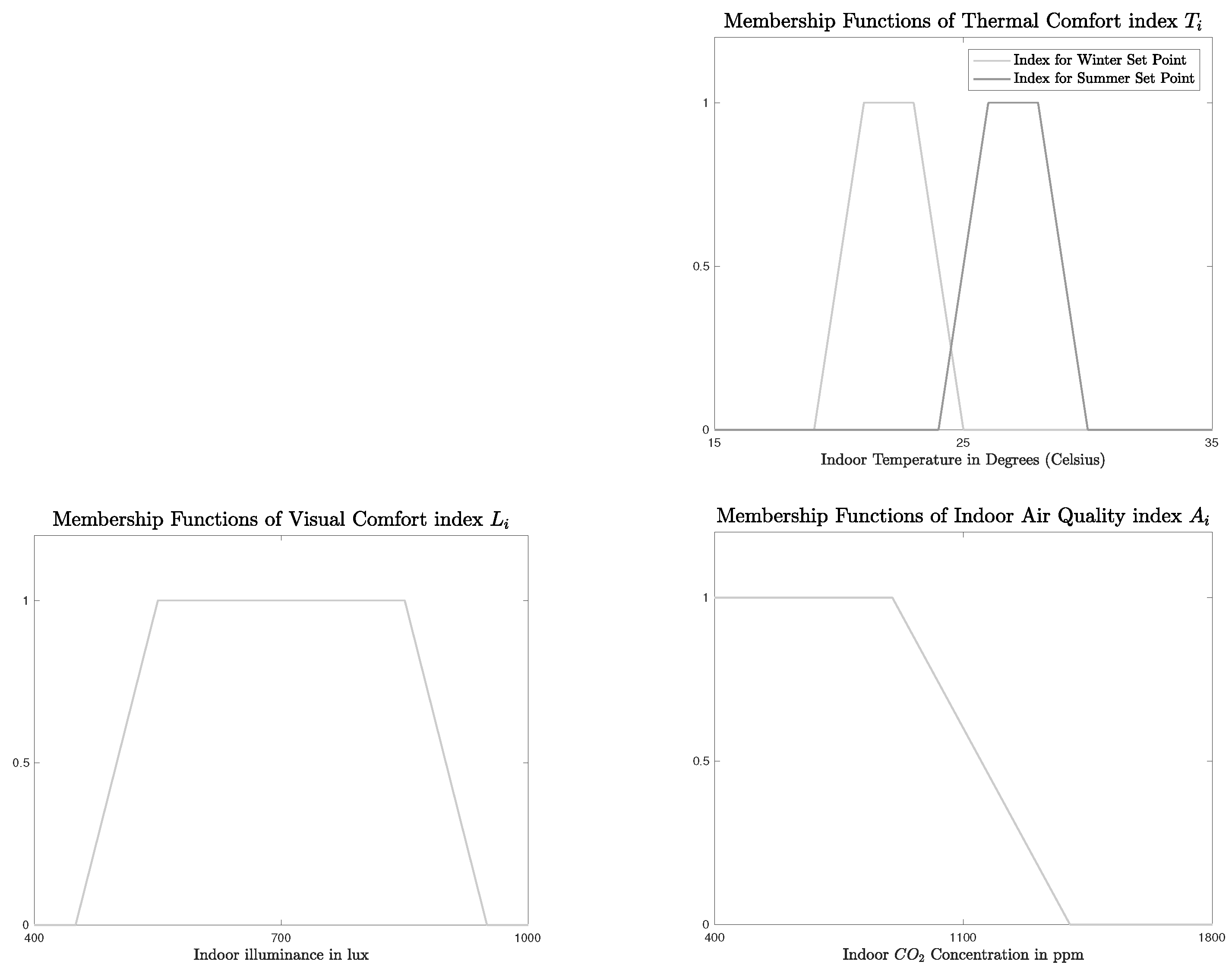
The overall comfort index
arises from three indexes; the thermal comfort index
, the visual comfort index
, and the indoor air quality index
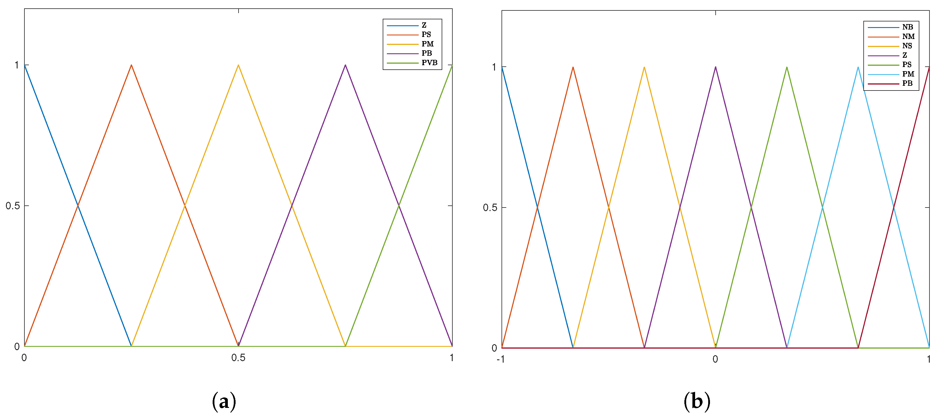
. The trapezoidal membership functions, that calculate the respecting indexes according to the indoor temperature, the indoor horizontal illuminance and the CO
2 concentration, are depicted in
Figure 18.
The overall comfort index is computed by the following equation:
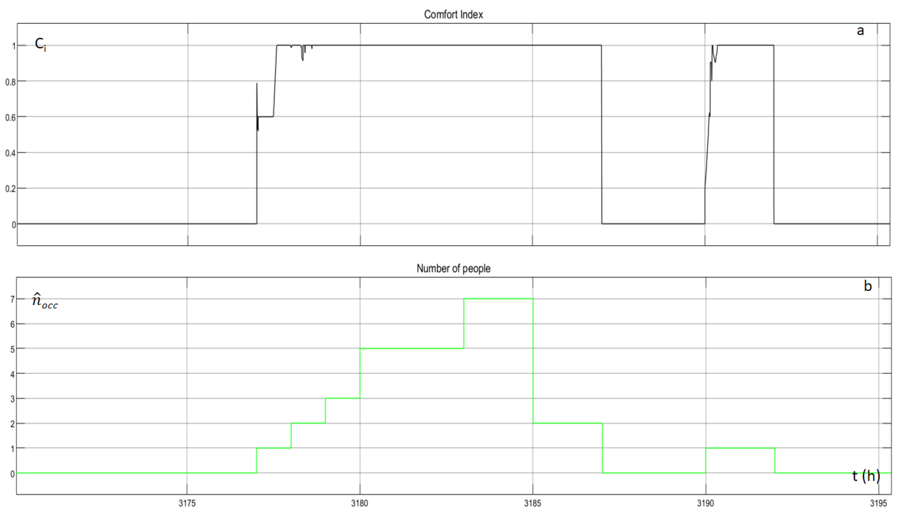
Figure 19 illustrates
and the number of occupants for a random day.
is zero when no occupants are inside the building and equals, for most of the time, to one when there are occupants inside the building.
The MACS performance, pertaining to the case of fuzzy parameters, is presented in the following figures.
Figure 20 and
Figure 21, illustrate the outdoor temperature, the indoor temperature, the control signal, and the occupancy level estimated when using
and
, respectively.
Figure 22 depicts the MACS results, associated with the occupancy estimation, pertaining to
. The outdoor illuminance, the total indoor illuminance, the control signal, the transparency of the window, the artificial lighting and the occupancy level, are illustrated. The results when using the
-based estimated occupancy vector, are given in
Figure 23.
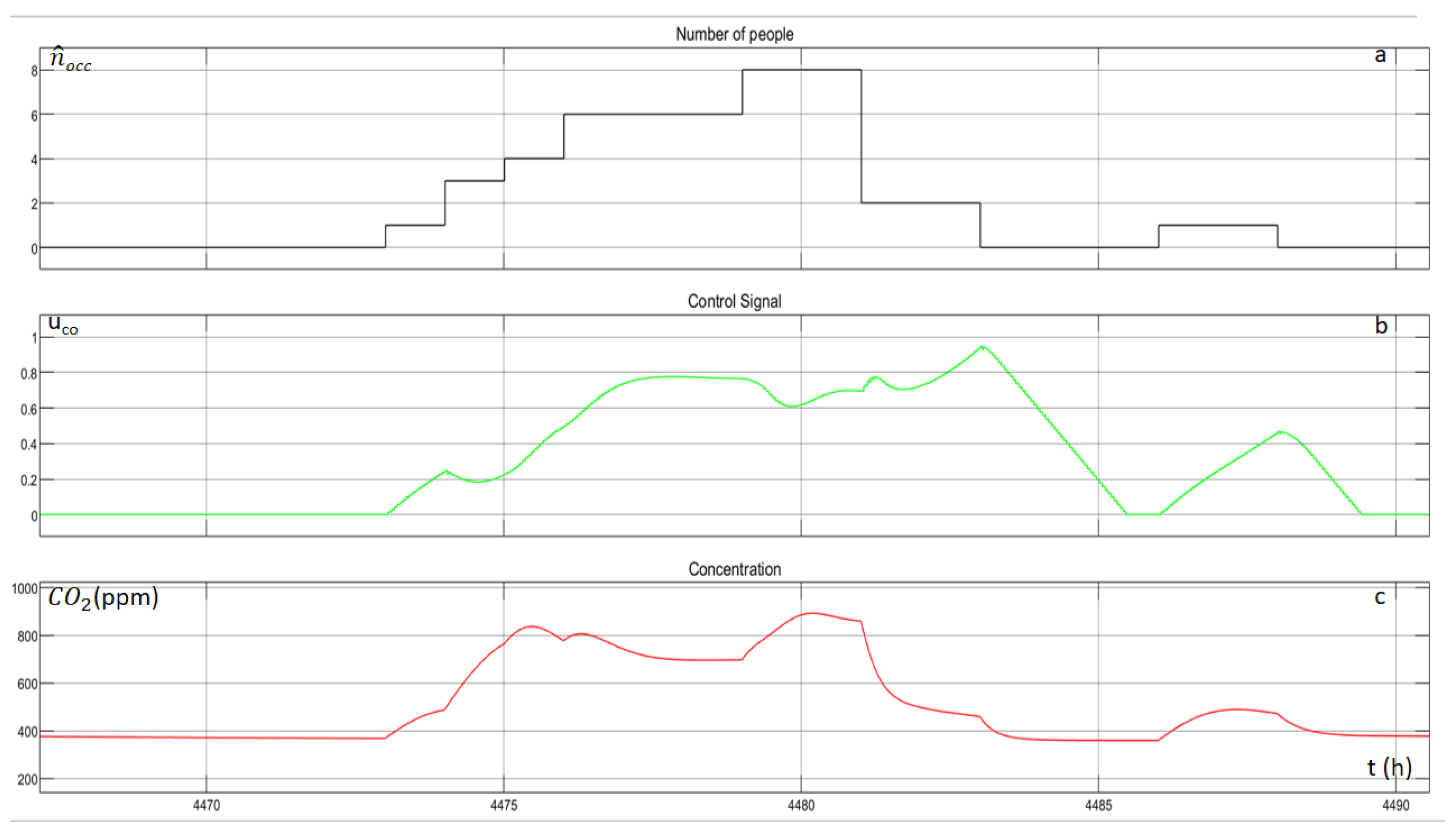
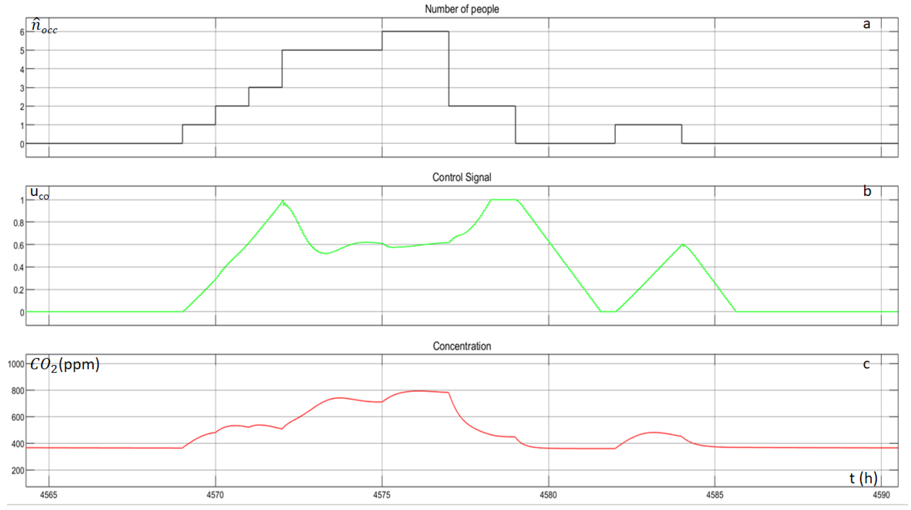
Figure 24 and
Figure 25, illustrate the occupancy of the building, the control signal of the agent and the indoor CO
2 concentration, for one random day for the different occupancy vectors.
The total consumption, as well as the consumptions of the heating/cooling system, the artificial lighting system and the ventilation system for two different occupancy profiles, are presented in
Table 6. In the first profile, the overall consumption is 1533 kWh, meaning a reduction of 130 kWh (Comparison with the first column of
Table 5). This reduction is a result of the ventilation system. The agent of the ventilation system learns a policy that reduces the consumption of the actuator but, as it is illustrated in
Figure 24, the indoor air of the building, is of lower quality, as the CO
2 concentration reaches values up to 900 ppm. Small reduction is also observed to the heating/cooling system (
Figure 20), but it is justified by the increased number of the occupants: More occupants are heating the thermal space, due to the occupant’s heating gains.
In the second profile, the overall consumptions is 1528 kWh, meaning a reduction of 135 kWh (Comparison with the first column of
Table 5). In this case, the reduction is a result from the heating/cooling system (
Figure 21). The agent of this system learns a better policy that reduces the consumption of the system, without particularly reducing the thermal comfort. A small reduction of 2 kWh is observed to the ventilation system (
Figure 25), which is justified by the lower number of the occupants. The consumption of the lighting system, as it is illustrated in
Figure 22 and
Figure 23, remains the same, since the lighting system is not affected by the occupant number.


