
The Implementation of Multiple Linear Regression for Swimming Pool Facilities: Case Study at Jøa, Norway

 , , , ,
  and
and 
Abstract
:
1. Introduction
1.1. Background
1.2. Motivation
1.3. Theoretical Background
1.4. Energy Prediction Methods
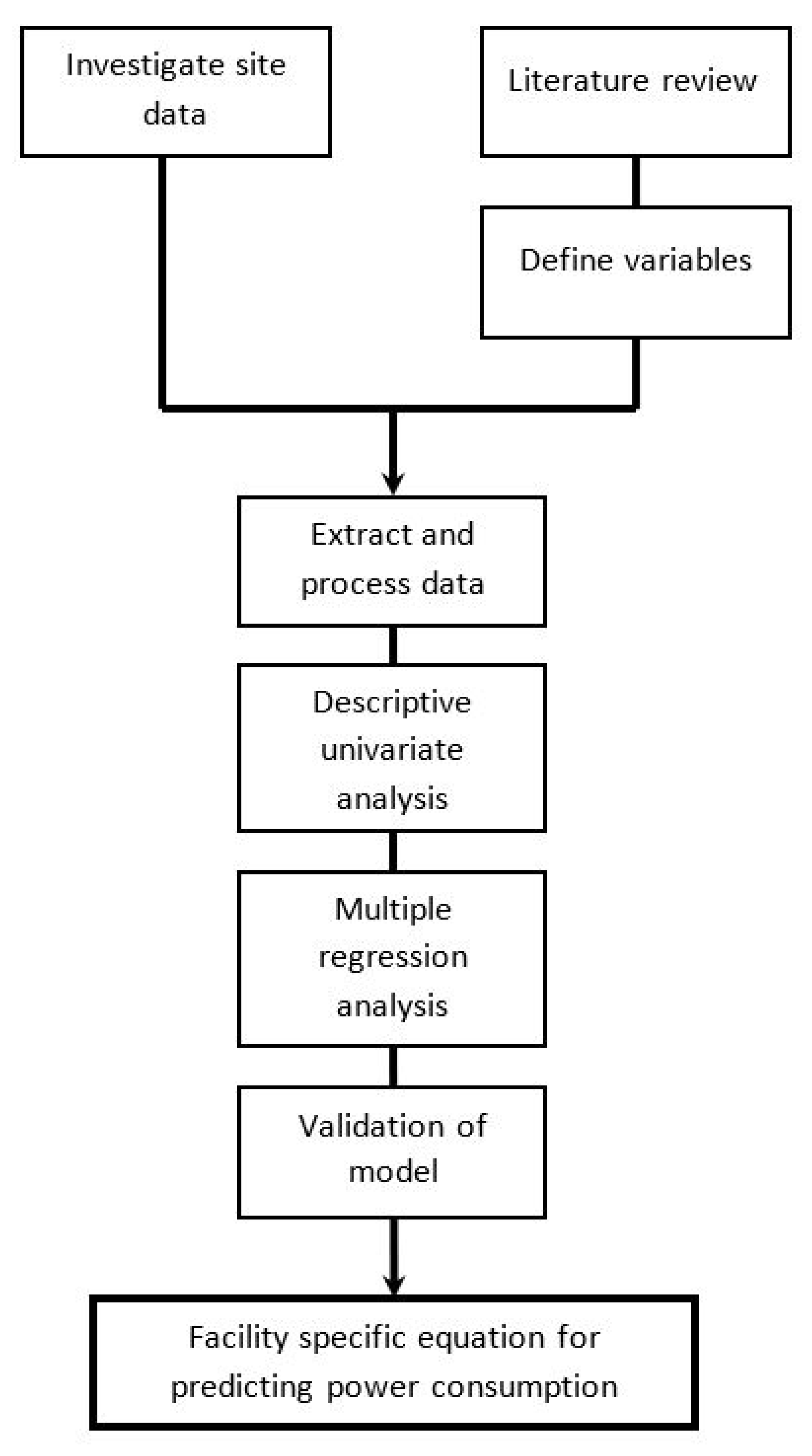
2. Method
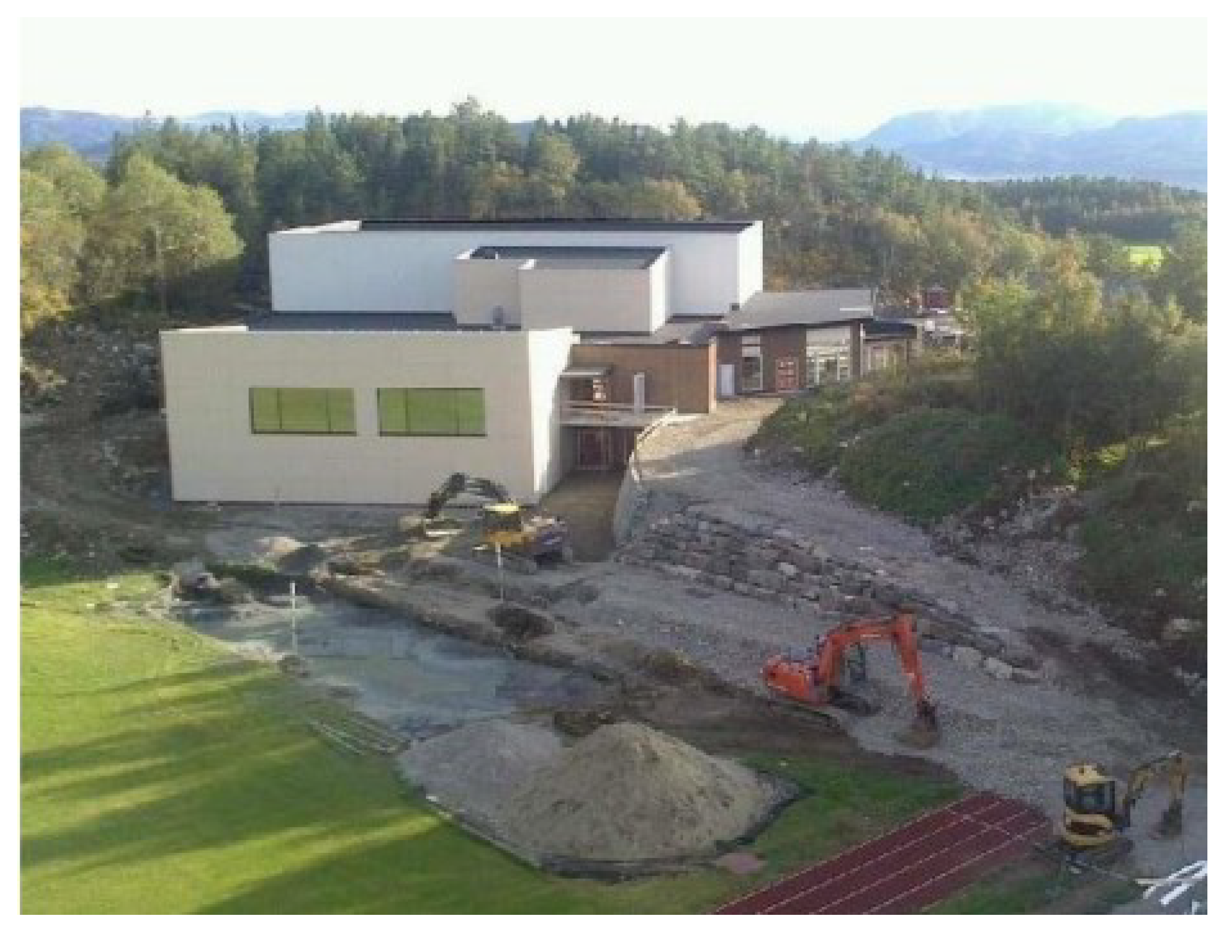
2.1. The Building
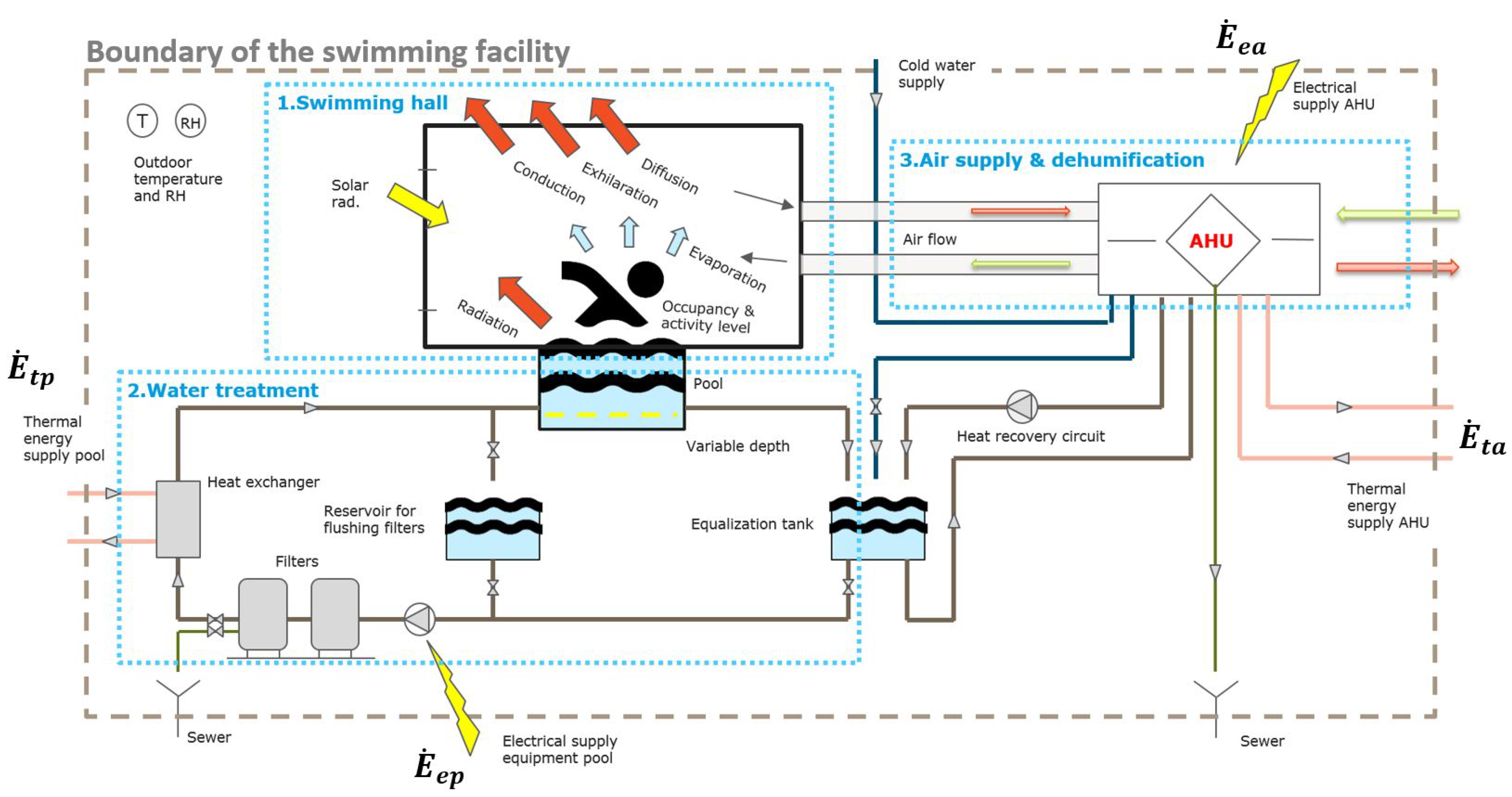
2.2. The Technical Systems
2.3. The Dataset
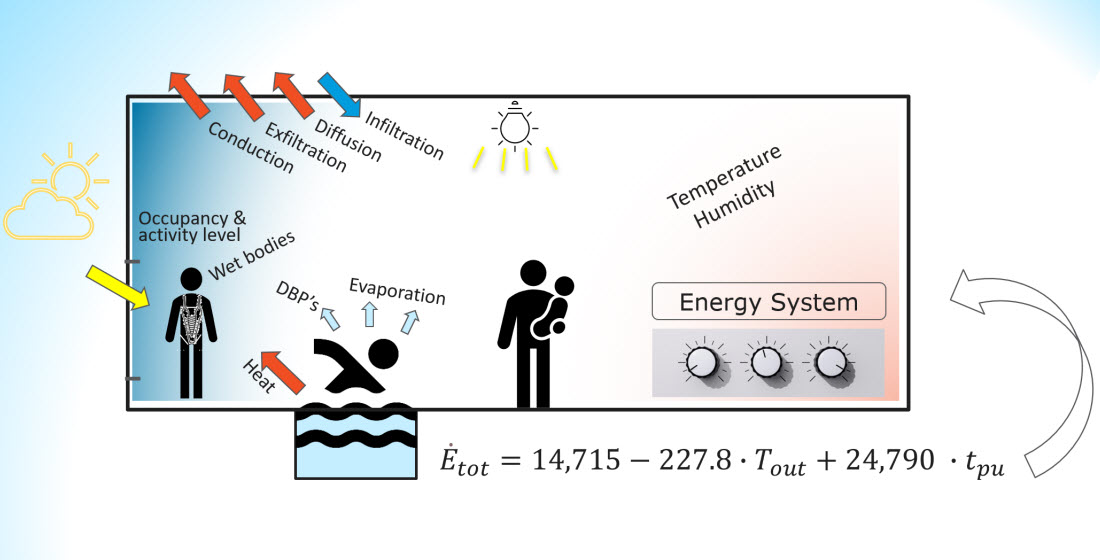
2.4. The Variables
- 1
- Extracting historic data from the BAS.
- 2
- Collecting weather data from the national database of the Norwegian Meteorological Institute [46].
- 3
- Digitalizing handwritten occupancy data due to lack of electronic occupancy registration.
- 4
- Calculating new variables based on indirectly monitored data. This is reported for the respective variables in Table 1.
Cleaning the Dataset
2.5. Statistical Methodology
2.5.1. Multiple Linear Regression
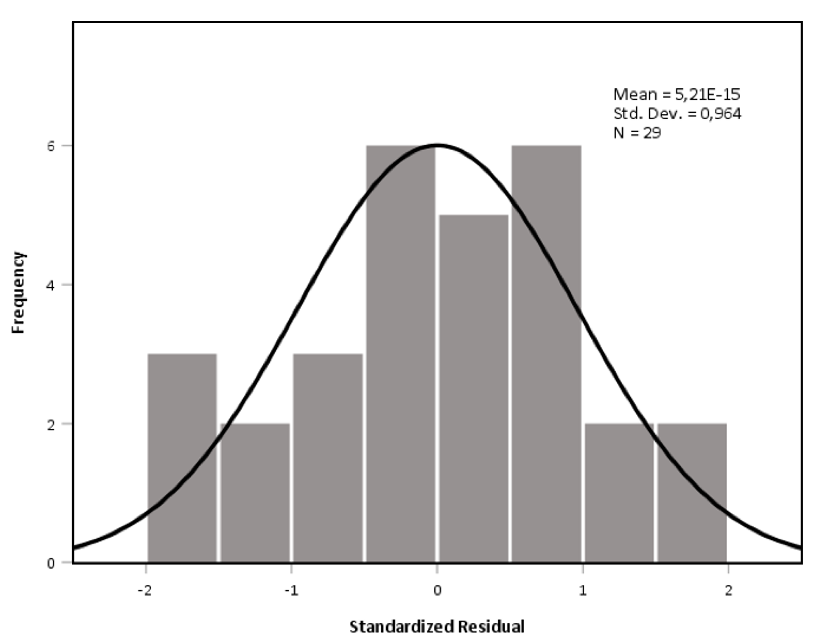
2.5.2. Assumptions
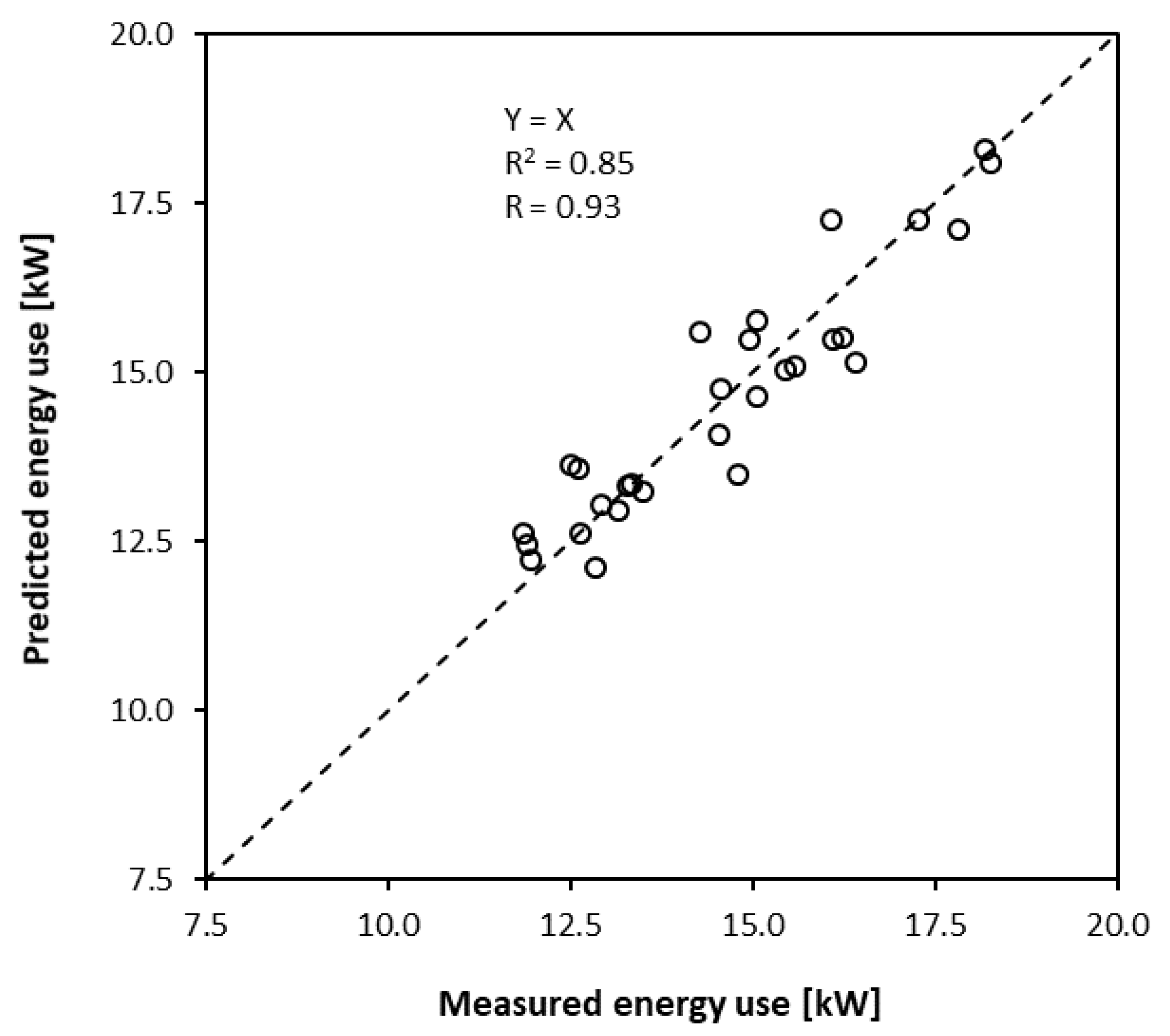
2.5.3. Evaluation of the Prediction Model
2.5.4. Validation
3. Results and Discussion
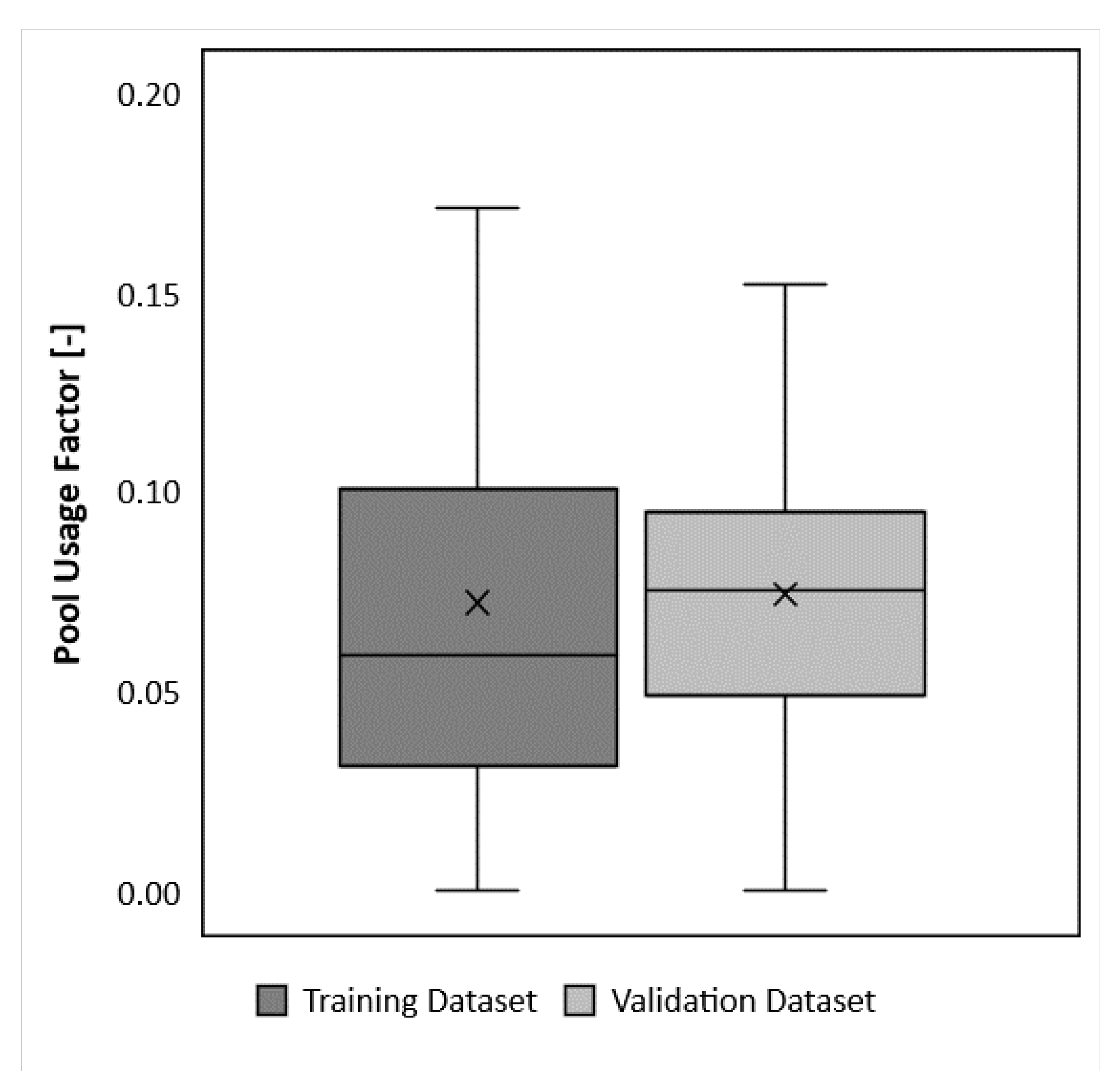
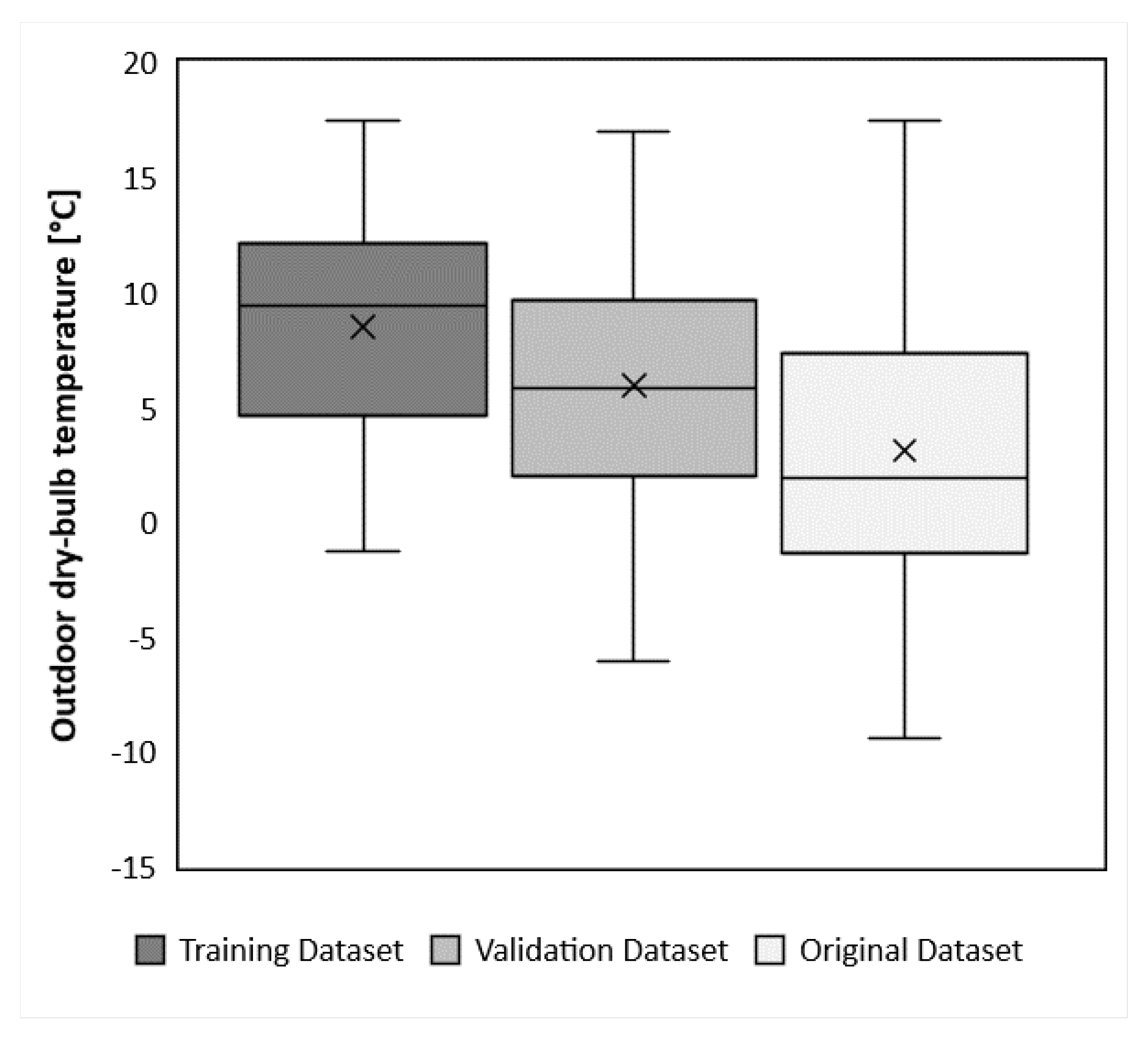
3.1. Description—The Training Dataset
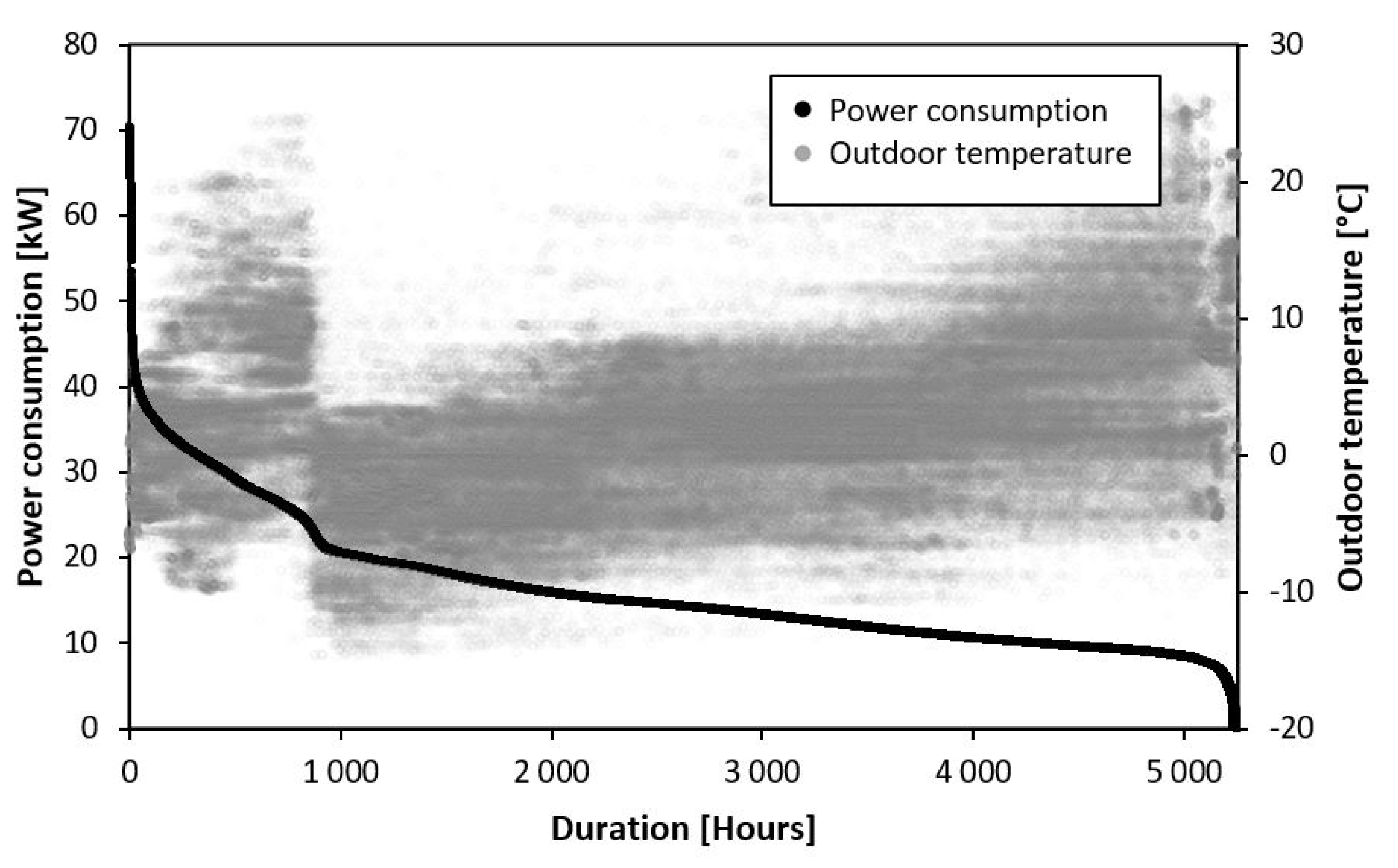
3.1.1. The Energy Performance of the Facility
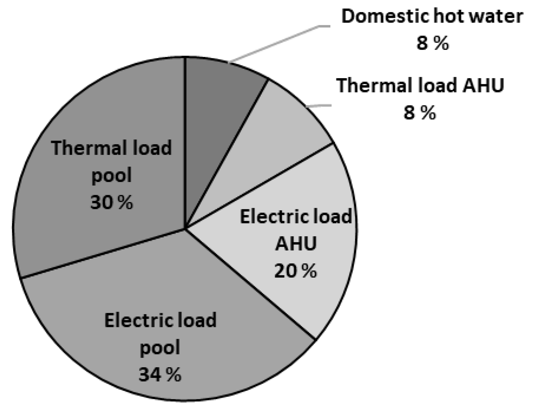
3.1.2. Energy Distribution
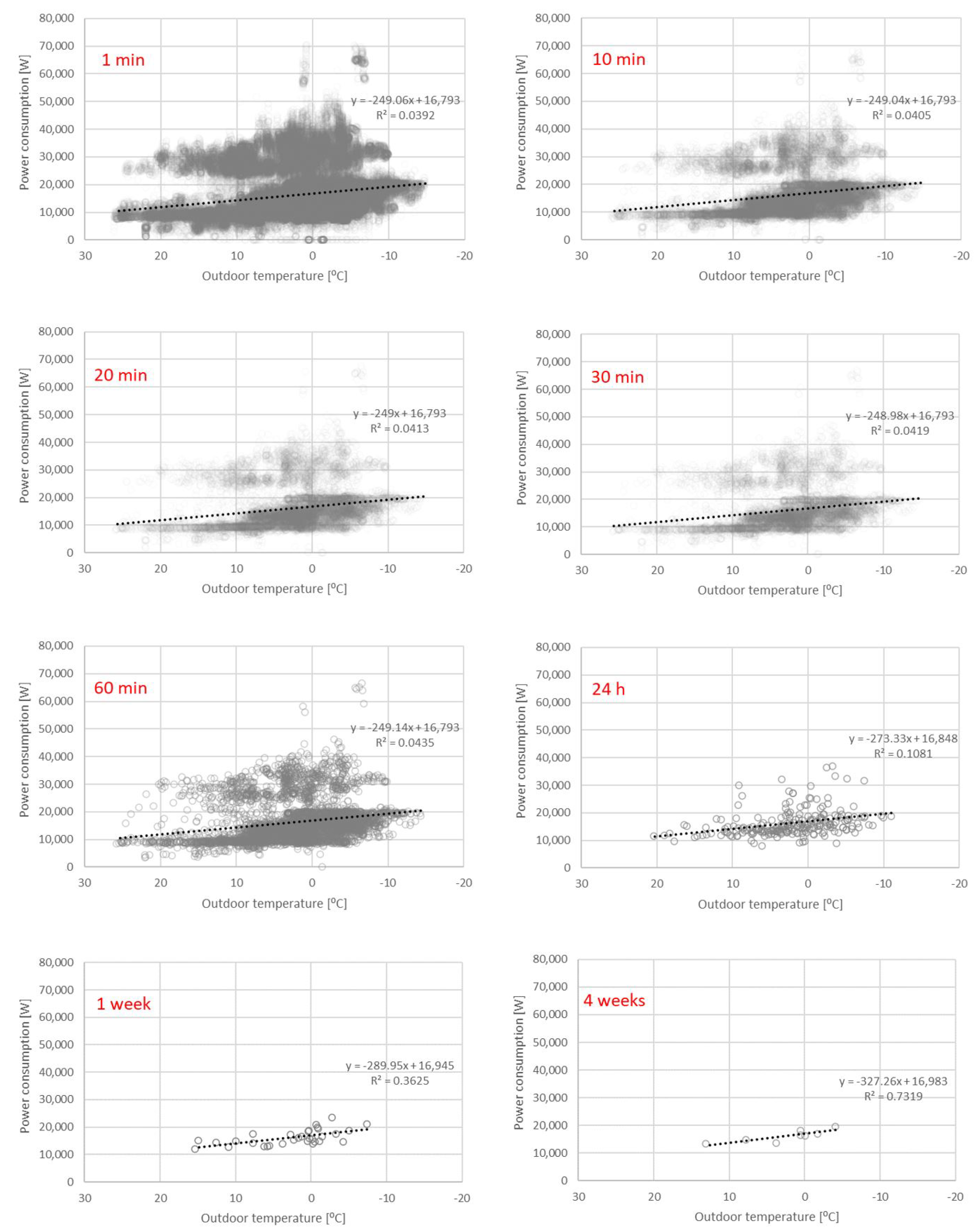
3.1.3. Time Step Analysis
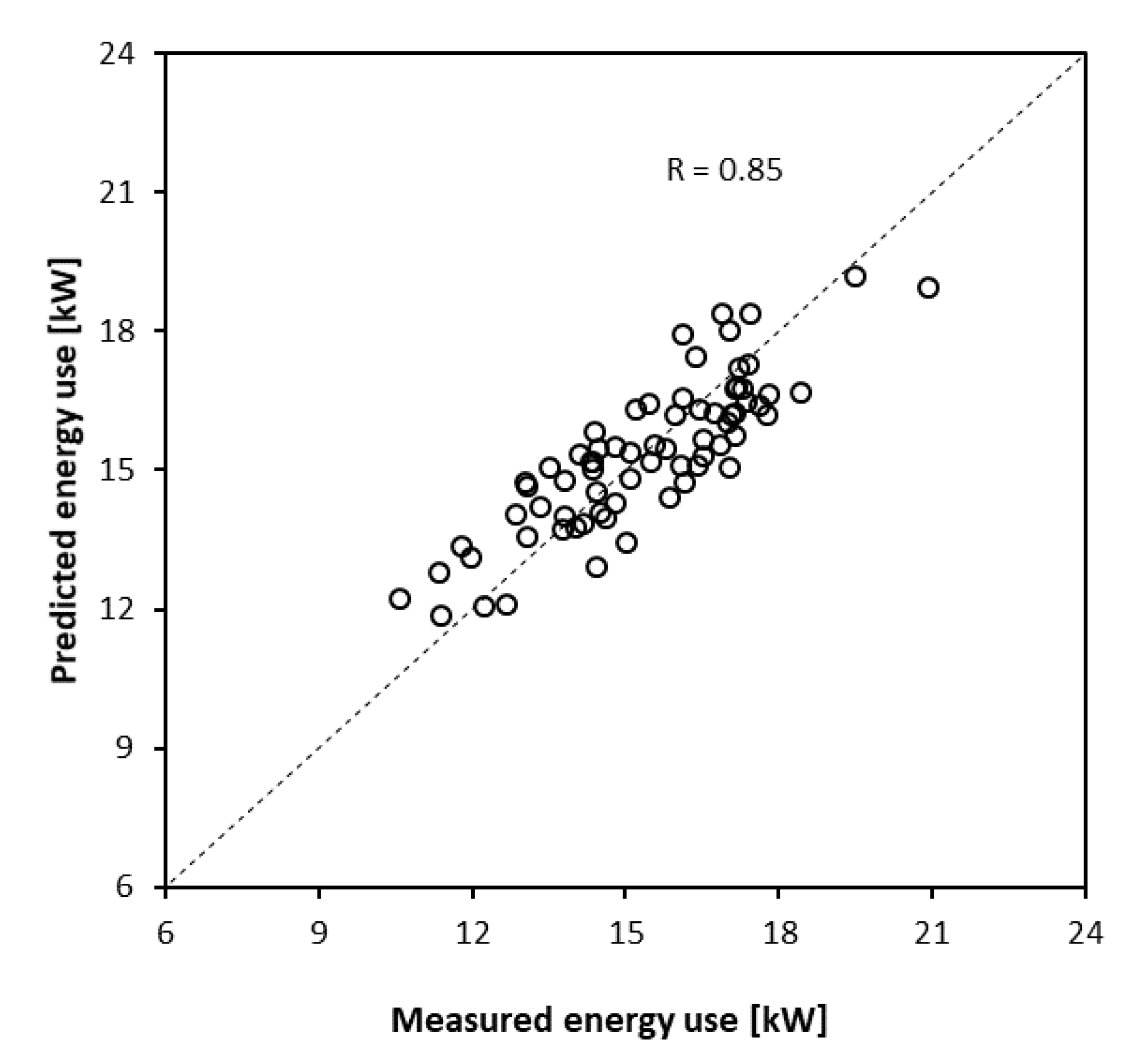
3.2. Statistical Analysis—Developing the Model
New Training Dataset
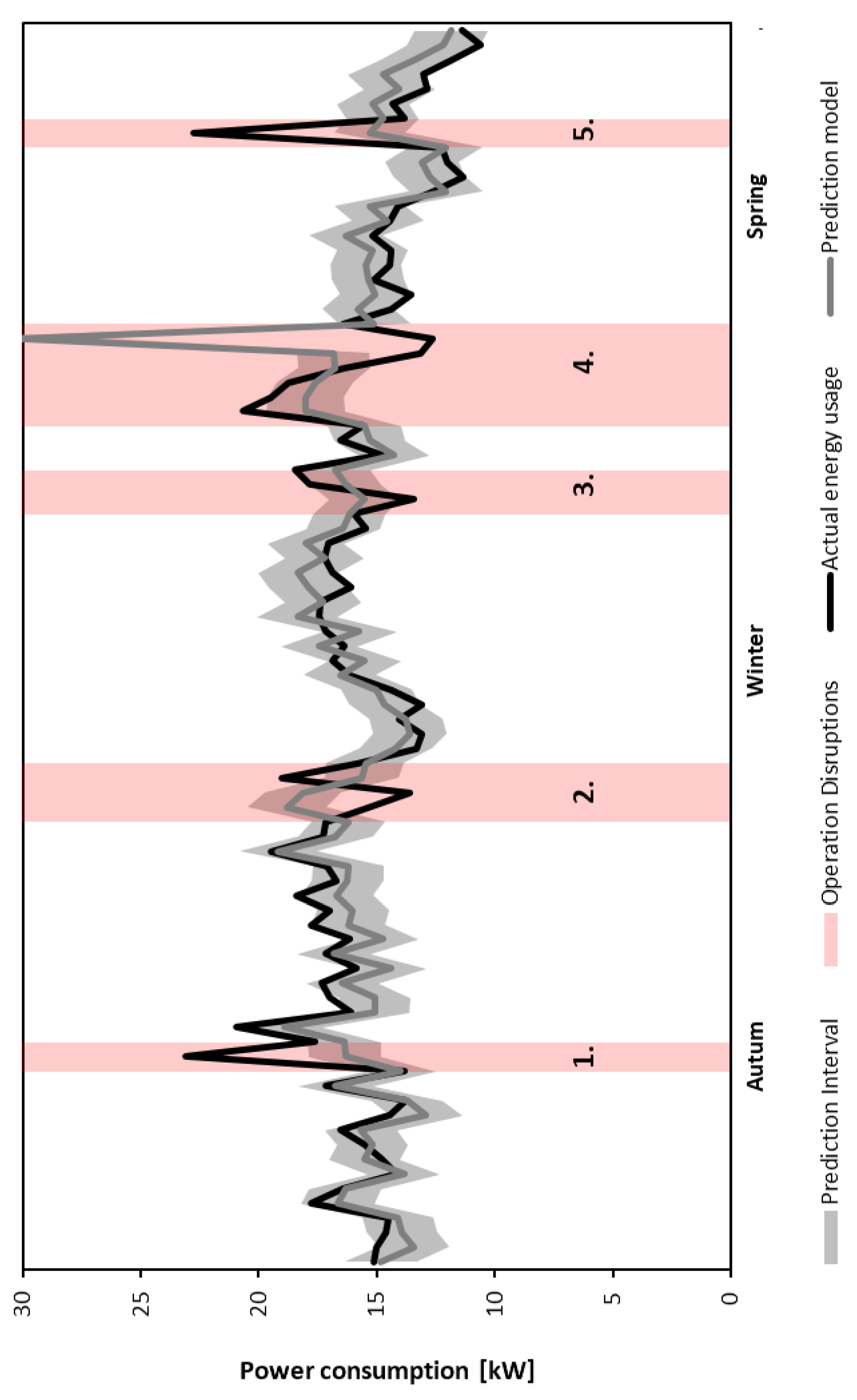
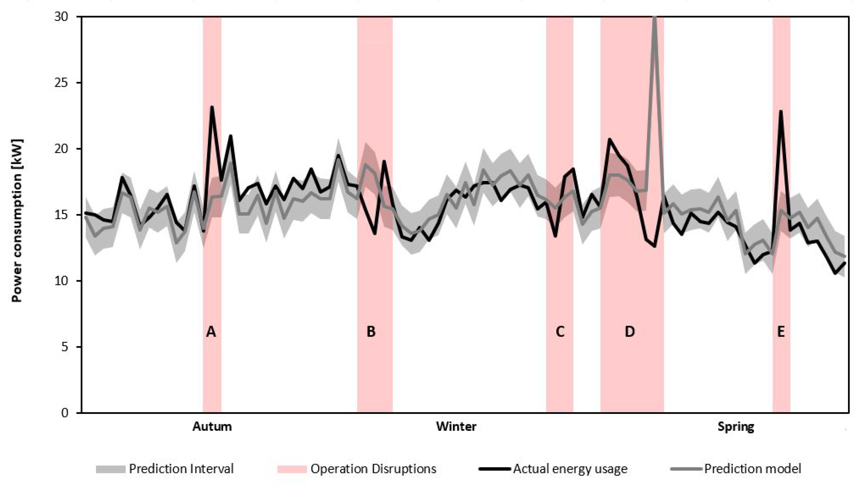
3.3. Validation and Application
4. Discussion and Opportunities for Deployment of the Created Model
5. Conclusions
- The study has shown that it is possible to develop an accurate energy prediction model for swimming facilities with a minimum of variables and datapoints.
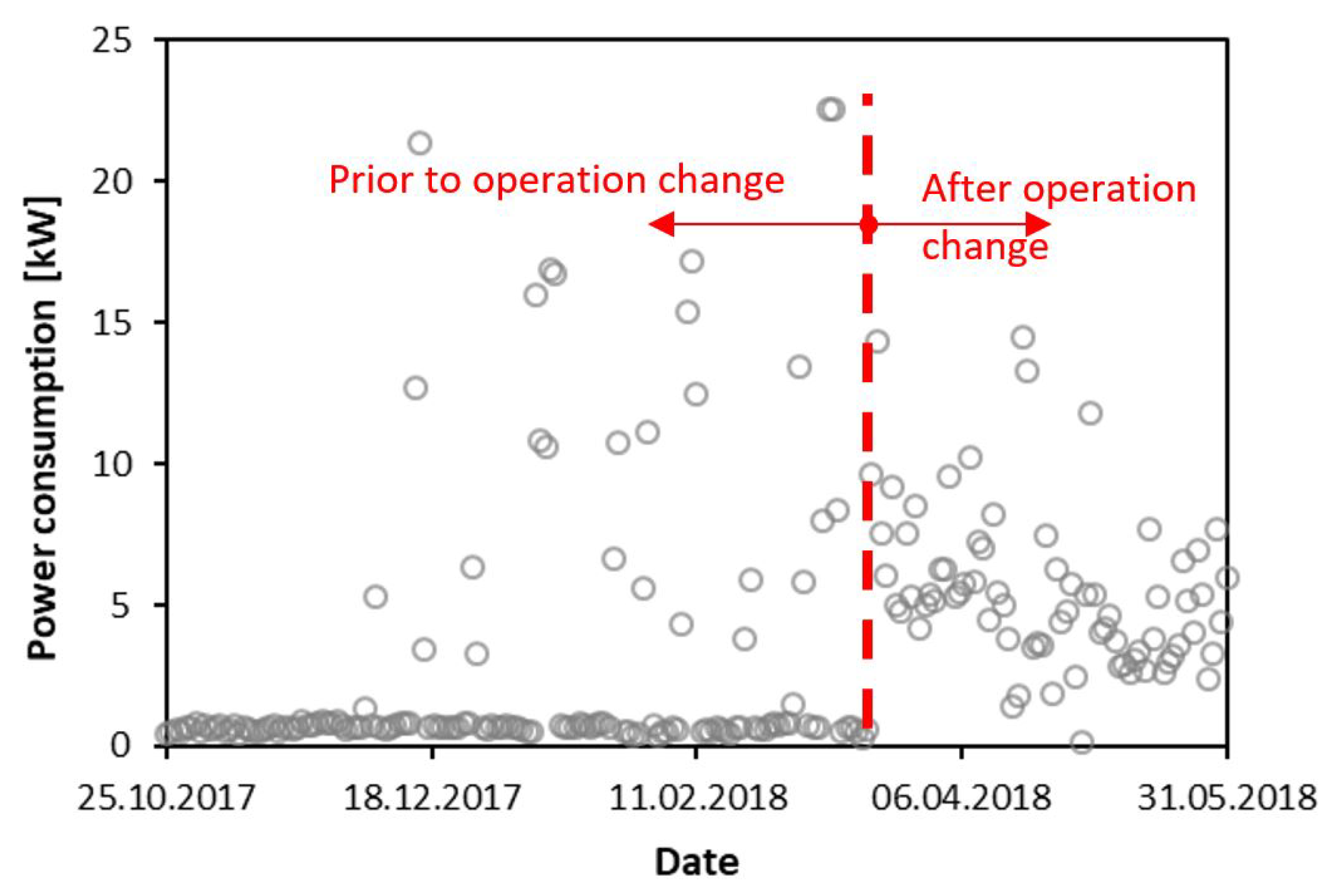
- The results from the analysis of the training dataset underlined the importance of investigating the training data prior to training of the model. The original dataset was based on raw data from 7 months of operation after the building was commissioned and approved by the building owner. The modified and preferred dataset was reduced after an in-depth investigation that revealed comprehensive operational disruptions. The final training dataset consisted of only 29 datapoints of 3-day averaged data ranging over a period of 3 months, March to June 2018.
- The statistically significant independent variables were found to be the outdoor dry-bulb temperature and the pool usage factor, which predicted the average power consumption accurately in the validation process. In the validation period from September 2018 to June 2019, the equation correctly identified all the critical operational disruptions.
- The model has been shown to be a suitable tool for helping operating staff in continuous evaluation of the energy performance of a facility and quickly disclosing possible operational disruptions. By identifying possible operational irregularities at an early stage, excessive energy use in operation can be avoided. Operational irregularities occur in a high percentage of new buildings. The importance of focusing on the operating phase and the overall energy consumption is crucial when minimizing the environmental impact. In addition, the knowledge of the energy performance of buildings is fundamental in achieving the energy targets. For swimming facilities, inappropriate operation of technical installations may also cause problems such as degradation of equipment and the occurrence of sick building syndrome.
- This study only investigated one specific facility and future work should address the robustness of the model and transferability to other swimming facilities.
Author Contributions
Funding
Institutional Review Board Statement
Informed Consent Statement
Data Availability Statement
Acknowledgments
Conflicts of Interest
Appendix A
Appendix B
| Subject | Quantity |
| Window surface area | 30 m |
| Water surface | 12.5 m × 8.5 m |
| Useable area | 266 m |
| Nominal air flow, air handling unit | 11,000 m/h |
| Nominal thermal power, air condenser | 26 kW |
| Nominal thermal power, pool water condenser | 34 kW |
| Nominal water flow circulation pool circuit | 60 m/h |
| Rating condition pool circuit | 300 visitors/day |
| Nominal power pool heater | 70 kW |
References
- Progress Made in Cutting Emissions. 2020. Available online: https://ec.europa.eu/clima/policies/strategies/progress_en (accessed on 15 April 2021).
- The European Green Deal. Available online: https://eur-lex.europa.eu/resource.html?uri=cellar:b828d165-1c22-11ea-8c1f-01aa75ed71a1.0002.02/DOC_1&format=PDF (accessed on 1 August 2021).
- Energy Roadmap 2050. Available online: https://eur-lex.europa.eu/LexUriServ/LexUriServ.do?uri=COM:2011:0885:FIN:EN:PDF (accessed on 1 August 2021).
- Ratajczak, K.; Szczechowiak, E. Energy consumption decreasing strategy for indoor swimming pools–Decentralized Ventilation system with a heat pump. Energy Build. 2020, 206, 109574. [Google Scholar] [CrossRef]
- Ratajczak, K.; Szczechowiak, E. The Use of a Heat Pump in a Ventilation Unit as an Economical and Ecological Source of Heat for the Ventilation System of an Indoor Swimming Pool Facility. Energies 2020, 13, 6695. [Google Scholar] [CrossRef]
- Kampel, W.; Aas, B.; Bruland, A. Energy-use in Norwegian swimming halls. Energy Build. 2013, 59, 181–186. [Google Scholar] [CrossRef]
- Kampel, W. Energy Efficiency in Swimming Facilities. 2015. Available online: https://ntnuopen.ntnu.no/ntnu-xmlui/handle/11250/2366793 (accessed on 20 November 2020).
- Røkenes, H. Betraktninger Rundt Svømmehallers Energieffektivitet. Master’s Thesis, Norwegian University of Science and Technology, Trondheim, Norway. 2011. [Google Scholar]
- Swim England. The Use of Energy in Swimming Pools. 2016. Available online: https://www.swimming.org/library/documents/1187/download (accessed on 24 March 2021).
- Rincón, L.; Castell, A.; Pérez, G.; Solé, C.; Boer, D.; Cabeza, L.F. Evaluation of the environmental impact of experimental buildings with different constructive systems using Material Flow Analysis and Life Cycle Assessment. Appl. Energy 2013, 109, 544–552. [Google Scholar] [CrossRef]
- Catrini, P.; Curto, D.; Franzitta, V.; Cardona, F. Improving energy efficiency of commercial buildings by Combined Heat Cooling and Power plants. Sustain. Cities Soc. 2020, 60, 102157. [Google Scholar] [CrossRef]
- GlobalABC/IEA/UNEP (Global Alliance for Buildings and Construction, International Energy Agency, and the United Nations Environment Programme). GlobalABC Roadmap for Buildings and Construction: Towards a Zero-Emission, Efficient and Resilient Buildings and Construction Sector; IEA: Paris, France, 2020. [Google Scholar]
- ASHRAE. Applications Handbook. American Society of Heating, Refrigerating and Air-Conditioning Engineers; ASHRAE: Atlanta, GA, USA, 2015. [Google Scholar]
- Smedegård, O.; Aas, B.; Stene, J.; Georges, L.; Carlucci, S. A Systematic and Data-Driven Literature Review on the Energy and Environmental Performance of Swimming Facilities. Unpublished work. 2021. [Google Scholar]
- Djuric, N. Real-Time Supervision of Building HVAC System Performance. 2008. Available online: https://ntnuopen.ntnu.no/ntnu-xmlui/handle/11250/231184 (accessed on 24 November 2020).
- Nord, N.; Novakovic, V.; Frydenlund, F. Kontinuerlig Funksjonskontroll for Effektiv Drift av Bygninger; SINTEF: Oslo, Norway, 2012. [Google Scholar]
- Ruparathna, R.; Hewage, K.; Sadiq, R. Developing a level of service (LOS) index for operational management of public buildings. Sustain. Cities Soc. 2017, 34, 159–173. [Google Scholar] [CrossRef] [Green Version]
- Saleem, S.; Haider, H.; Hu, G.; Hewage, K.; Sadiq, R. Performance indicators for aquatic centres in Canada: Identification and selection using fuzzy based methods. Sci. Total Environ. 2021, 751, 141619. [Google Scholar] [CrossRef]
- Berardi, U. Sustainability assessment in the construction sector: Rating systems and rated buildings. Sustain. Dev. 2012, 20, 411–424. [Google Scholar] [CrossRef]
- The Norwegian Ministry of Petroleum and Energy. Energy Labelling Regulations for Buildings. 2010. Available online: https://lovdata.no/dokument/SF/forskrift/2009-12-18-1665 (accessed on 25 November 2020).
- NS 3700. Criteria for Passive Houses and Low Energy Houses: Residential Buildings (Original: Kriterier for Passivhus og Lavenergihus: Boligbyginger). 2013. Available online: https://www.standard.no/no/nettbutikk/produktkatalogen/Produktpresentasjon/?ProductID=636902 (accessed on 15 November 2020).
- NS 3701. Criteria for Passive Houses and Low Energy Buildings-Non-Residential Buildings. 2012. Available online: https://www.standard.no/no/Nettbutikk/produktkatalogen/Produktpresentasjon/?ProductID=587802 (accessed on 15 November 2020).
- Duverge, J.J.; Rajagopalan, P.; Fuller, R. Defining aquatic centres for energy and water benchmarking purposes. Sustain. Cities Soc. 2017, 31, 51–61. [Google Scholar] [CrossRef]
- Zhao, H.X.; Magoulès, F. A review on the prediction of building energy consumption. Renew. Sustain. Energy Rev. 2012, 16, 3586–3592. [Google Scholar] [CrossRef]
- Lu, T.; Lü, X.; Viljanen, M. A new method for modeling energy performance in buildings. Energy Procedia 2015, 75, 1825–1831. [Google Scholar] [CrossRef]
- Westerlund, L.; Dahl, J.; Johansson, L. A theoretical investigation of the heat demand for public baths. Energy 1996, 21, 731–737. [Google Scholar] [CrossRef]
- Lovell, D.; Rickerby, T.; Vandereydt, B.; Do, L.; Wang, X.; Srinivasan, K.; Chua, H. Thermal performance prediction of outdoor swimming pools. Build. Environ. 2019, 160, 106167. [Google Scholar] [CrossRef]
- Klein, S.; Beckman, W.; Mitchell, J.; Duffie, J.; Duffie, N.; Freeman, T.; Braun, J.; Evans, B. TRNSYS 18. A TRaNsient SYstem Simulation Program; Standard Component Library 515 Overview; Solar Energy Laboratory; University of Wisconsin-Madison: Madison, WI, USA, 2017; Volume 3, p. 516. [Google Scholar]
- Energy Systems Research Unit (ESRU). The ESP-r System for Building Energy Simulation: User Guide Version 10 Series. Available online: www.esru.strath.ac.uk/Documents/ESP-ruserguide.pdf (accessed on 15 April 2021).
- EQUA Simulation AB. Building Performance—Simulation Software EQUA 2020. Available online: www.equa.se (accessed on 15 April 2021).
- Mančić, M.V.; Živković, D.S.; Milosavljević, P.M.; Todorović, M.N. Mathematical modelling and simulation of the thermal performance of a solar heated indoor swimming pool. Therm. Sci. 2014, 18, 999–1010. [Google Scholar] [CrossRef] [Green Version]
- Mančić, M.V.; Živković, D.S.; Đorđević, M.L.; Jovanović, M.S.; Rajić, M.N.; Mitrović, D.M. Techno-economic optimization of configuration and capacity of a polygeneration system for the energy demands of a public swimming pool building. Therm. Sci. 2018, 22, 1535–1549. [Google Scholar] [CrossRef] [Green Version]
- Duverge, J.J.; Rajagopalan, P. Assessment of factors influencing the energy and water performance of aquatic centres. Build. Simul. 2020, 13, 771–786. [Google Scholar] [CrossRef]
- Yuce, B.; Li, H.; Rezgui, Y.; Petri, I.; Jayan, B.; Yang, C. Utilizing artificial neural network to predict energy consumption and thermal comfort level: An indoor swimming pool case study. Energy Build. 2014, 80, 45–56. [Google Scholar] [CrossRef]
- Kampel, W.; Carlucci, S.; Aas, B.; Bruland, A. A proposal of energy performance indicators for a reliable benchmark of swimming facilities. Energy Build. 2016, 129, 186–198. [Google Scholar] [CrossRef]
- Duverge, J.J.; Rajagopalan, P.; Fuller, R.; Woo, J. Energy and water benchmarks for aquatic centres in Victoria, Australia. Energy Build. 2018, 177, 246–256. [Google Scholar] [CrossRef]
- Gassar, A.A.A.; Cha, S.H. Energy prediction techniques for large-scale buildings towards a sustainable built environment: A review. Energy Build. 2020, 224, 110238. [Google Scholar] [CrossRef]
- Safa, M.; Safa, M.; Allen, J.; Shahi, A.; Haas, C.T. Improving sustainable office building operation by using historical data and linear models to predict energy usage. Sustain. Cities Soc. 2017, 29, 107–117. [Google Scholar] [CrossRef]
- Safa, M.; Allen, J.; Safa, M. Predicting energy usage using historical data and linear models. In Proceedings of the International Symposium on Automation and Robotics in Construction, Sydney, Australia, 9–11 July 2014; IAARC Publications: Sydney, Australia, 2014; Volume 31, p. 1. [Google Scholar]
- Catalina, T.; Virgone, J.; Blanco, E. Development and validation of regression models to predict monthly heating demand for residential buildings. Energy Build. 2008, 40, 1825–1832. [Google Scholar] [CrossRef]
- Catalina, T.; Iordache, V.; Caracaleanu, B. Multiple regression model for fast prediction of the heating energy demand. Energy Build. 2013, 57, 302–312. [Google Scholar] [CrossRef]
- Köppen, W.; Geiger, R. Handbuch der Klimatologie; Gebrüder Bornträger: Berlin, Germany, 1930. [Google Scholar]
- Johansson, L.; Westerlund, L. Energy savings in indoor swimming-pools: Comparison between different heat-recovery systems. Appl. Energy 2001, 70, 281–303. [Google Scholar] [CrossRef]
- Skibinski, B.; Uhlig, S.; Müller, P.; Slavik, I.; Uhl, W. Impact of different combinations of water treatment processes on the concentration of disinfection byproducts and their precursors in swimming pool water. Environ. Sci. Technol. 2019, 53, 8115–8126. [Google Scholar] [CrossRef]
- Novakovic, V.; Hanssen, S.; Thue, J.; Wangensteen, I.; Gjerstad, F. Enøk i bygninger-Effektiv energibruk. Oslo Gyldendal Undervis. 2007, 63, 327–361. [Google Scholar]
- Meteorologisk Institutt. eKlima 2018. Available online: www.eklima.no (accessed on 15 April 2021).
- Henley, A.; Wolf, D. Learn Data Analysis with Python; Lessons in Coding; Apress: New York, NY, USA, 2018. [Google Scholar]
- IBM Corp Ibm Statistics. Statistics for Windows, Version 25.0; IBM Corp.: Armonk, NY, USA, 2017. [Google Scholar]
- Box, G.; Jenkins, G.; Reinsel, G.; Ljung, G. Time Series Analysis, Control, and Forecasting; John Wiley & Son: Hoboken, NJ, USA, 2015. [Google Scholar]
- Eikemo, T.A.; Clausen, T.H. Kvantitativ Analyse med SPSS: En Praktisk Innføring i Kvantitative Analyseteknikker; Tapir Akademisk Forlag: Trondheim, Norway, 2012. [Google Scholar]
- NTNU Senter for Idrettsanlegg og Teknologi. Kunnskapsportalen for Idretts- og Nærmiljøanlegg Trondheim. 2020. Available online: https://www.godeidrettsanlegg.no/nyhet/energibruk-i-norske-svommehaller (accessed on 15 April 2021).
- Harrell, F.E., Jr. Regression Modeling Strategies: With Applications to Linear Models, Logistic and Ordinal Regression, and Survival Analysis; Springer: New York, NY, USA, 2015. [Google Scholar]
- Hanssen, S.O.; Mathisen, H.M. Evaporation from swimming pools. In Proceedings of the Roomvent ‘90, Oslo, Norway, 13–15 June 1990. [Google Scholar]
- Cornaro, C.; Buratti, C. Energy efficiency in buildings and innovative materials for building construction. Appl. Sci. 2020, 10, 2866. [Google Scholar] [CrossRef] [Green Version]
- Wu, L.; Kaiser, G.; Solomon, D.; Winter, R.; Boulanger, A.; Anderson, R. Improving efficiency and reliability of building systems using machine learning and automated online evaluation. In Proceedings of the 2012 IEEE Long Island Systems, Applications and Technology Conference (LISAT), Farmingdale, NY, USA, 4 May 2012; pp. 1–6. [Google Scholar]
- Pietkun-Greber, I.; Suszanowicz, D. The consequences of the inappropriate use of ventilation systems operating in indoor swimming pool conditions-analysis. In Proceedings of the E3S Web of Conferences, EDP Sciences, Krakow, 7–8 June 2018; Volume 45, p. 00064. [Google Scholar]
- Ciulla, G.; D’Amico, A. Building energy performance forecasting: A multiple linear regression approach. Appl. Energy 2019, 253, 113500. [Google Scholar] [CrossRef]
- Bataineh, K.M. Transient Analytical Model of a Solar-Assisted Indoor Swimming Pool Heating System. J. Energy Eng. 2015, 141, 04014048. [Google Scholar] [CrossRef]


| N | Variable | Unit | Type | Source | Comment |
|---|---|---|---|---|---|
| Ėea | Electric energy consumption, AHU | Dependent | BAS | Fans, compressor, pumps and control system | |
| Ėta | Thermal energy consumption, AHU | BAS | Supplied thermal energy for air heating | ||
| Ėep | Electric energy consumption, pool circuit | BAS | Related to pumps, disinfection, etc. | ||
| Ėtp | Thermal energy consumption, pool circuit | BAS | Supplied thermal energy for pool heating | ||
| Ėtot | Total thermal and electric energy consumption | Calculated | Summarized load pt. 1–4 | ||
| Outdoor dry-bulb temperature | °C | Independent | BAS | Measurement from the site | |
| Moisture content outdoor air | Calculated | Meteorological data | |||
| Enthalpy difference indoor/outdoor | Calculated | Combining meteorological data and indoor air measurements and by applying the ideal gas law | |||
| Pool usage factor (proportion of time the pool was in use) | - | BAS/Calculated | Calculated by utilizing water level data in the equalization tank | ||
| Number of adults bathing | adults | Handwritten | Manually digitalized and implemented in the dataset | ||
| Number of children bathing | children | Handwritten | Manually digitalized and implemented in the dataset | ||
| Water supply flow rate to the pool circuit | BAS/Calculated | Calculated by utilizing water level data, flushing reservoir |
| Unstandardized Coefficients | |||||
|---|---|---|---|---|---|
| B | Error | Standardized Coefficients | T | Significance | |
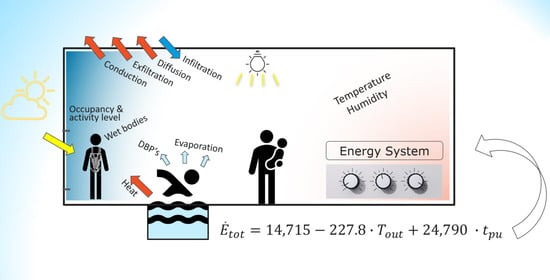
| Constant | 14,715 | 2410.7 | 16.387 | ||
| Outdoor temperature | −227.8 | 27.2 | −0.591 | −8.38 | 0.000 |
| Pool usage | 24,790 | 2607.5 | 0.671 | 9.507 | 0.000 |
Publisher’s Note: MDPI stays neutral with regard to jurisdictional claims in published maps and institutional affiliations. |
© 2021 by the authors. Licensee MDPI, Basel, Switzerland. This article is an open access article distributed under the terms and conditions of the Creative Commons Attribution (CC BY) license (https://creativecommons.org/licenses/by/4.0/).
Share and Cite
Smedegård, O.Ø.; Jonsson, T.; Aas, B.; Stene, J.; Georges, L.; Carlucci, S. The Implementation of Multiple Linear Regression for Swimming Pool Facilities: Case Study at Jøa, Norway. Energies 2021, 14, 4825. https://doi.org/10.3390/en14164825
Smedegård OØ, Jonsson T, Aas B, Stene J, Georges L, Carlucci S. The Implementation of Multiple Linear Regression for Swimming Pool Facilities: Case Study at Jøa, Norway. Energies. 2021; 14(16):4825. https://doi.org/10.3390/en14164825
Chicago/Turabian StyleSmedegård, Ole Øiene, Thomas Jonsson, Bjørn Aas, Jørn Stene, Laurent Georges, and Salvatore Carlucci. 2021. "The Implementation of Multiple Linear Regression for Swimming Pool Facilities: Case Study at Jøa, Norway" Energies 14, no. 16: 4825. https://doi.org/10.3390/en14164825
APA StyleSmedegård, O. Ø., Jonsson, T., Aas, B., Stene, J., Georges, L., & Carlucci, S. (2021). The Implementation of Multiple Linear Regression for Swimming Pool Facilities: Case Study at Jøa, Norway. Energies, 14(16), 4825. https://doi.org/10.3390/en14164825