Automatic Identification of Internal Wave Characteristics Affecting Bathymetric Measurement Based on Multibeam Echosounder Water Column Data Analysis

Abstract

The accuracy of multibeam echosounder bathymetric measurement depends on the accuracy of the data of the sound speed layers within the water column. This is necessary for the correct modeling of ray bending. It is assumed that the sound speed layers are horizontal and static, according to the sound speed profile traditionally used in the depth calculation. In fact, the boundaries between varying water masses can be curved and oscillate. It is difficult to assess the parameters of these movements based on the sparse sampling of sound velocity profiles (SVP) collected through a survey; thus, alternative or augmented methods are needed to obtain information about water mass stratification for the time of a particular ping or a series of pings. The process of water column data collection and analysis is presented in this paper. The proposed method updates the sound speed profile by the automated detection of varying water mass boundaries, giving the option to adjust the SVP for each beam separately. This can increase the overall accuracy of a bathymetric survey and provide additional oceanographic data about the study area.

1. Introduction

One of the essential components of every bathymetric survey is the measurement of the sound speed value, which is necessary to calculate the depths based on the two-way travel time of an acoustic signal sent from the echosounder and reflected back from seabed features. In the case of a multibeam echosounder (MBES), not only is the mean value of the sound speed of great importance, but also the data about water column stratification, which are used to estimate the refraction of outer beams. This requires the measurement of the sound velocity profile (SVP), using SVPs (sound velocity profilers—direct measurement) or CTD (conductivity, temperature, depth—indirect measurement) devices, which are lowered down from the sea surface to the seabed and measure the sound speed during downward and upward travel. This option requires a vessel to stop and stay in a drift for the period of the SVP measurement. There is also an option to use an MVP (moving vessel profiler), which does not need a vessel to stop, but requires dedicated, high-cost equipment on-board to automatically release and recover the MVP.

Both options of sound speed measurements are based on a discrete sampling of water stratification in time and space (measurement along a straight or close-to-straight line from the surface to seabed). The measured values indicate the parameters of the stratified water mass, and the boundaries between those masses are assumed to be straight and horizontal. This is the assumption of the ray tracing for oblique acoustic rays. The basic methods used to calculate the distance traveled by the signal during a measured time assumes the layers have a constant sound speed. The horizontal components of the traveled distance through each of the layers are calculated using Snell’s law. The accuracy of this solution is determined by the number of layers. Another method is based upon layers with a constant sound speed gradient. Within each of these layers, the ray path has a constant curvature. Again, the distances in each layer are summed until half of the two-way travel time is reached, taking the circular ray path within the layer into account. Both methods are based on the assumption that the water mass boundaries are straight and horizontal [1]. These assumptions are used during the depth calculations of multibeam echosounder measurements. A significant source of error can, however, be introduced here, because these boundaries can not only be curved but also can oscillate [2]. This movement is described as the internal wave phenomenon. According to [2], a total propagated depth uncertainty can even exceed the IHO Order 1A/B specifications due to internal waves.

The measurement of the internal wave (IW) parameters is a problematic task because the measurement techniques practically used today allow only the sampling of the water mass with a particular measuring sampling frequency that is insufficient to estimate the unknown values. Direct measurements can, however, be augmented by the visualization of the acoustic response from a single beam or multibeam echosounder signal sent through the water column.

The assessment of the possibilities of using multibeam echosounder water column data for the delimitation of differing water masses for the time of a particular depth measurement is presented in this paper. The data were collected in the highly stratified estuary of Mobile Bay, at the mouth of the Mobile River, Alabama, United States, with a Sonic 2024 multibeam echosounder, processed using Qimera and Fledermaus Midwater software by QPS (Quality Positioning Services) and analyzed with the use of Matlab scripts.

2. Fundamentals

The character of the analyzed phenomena, as described in this section, and the way the raw data are obtained determine the analysis methods used.

2.1. Internal Wave Phenomenon

The internal wave is a phenomenon that occurs on the continental shelf, in the oceans below the surface of the sea. Internal waves are observed within the stratified water column in coastal waters, straits, and lakes [3,4,5]. IWs may be considered as density oscillations that propagate up to several hundred kilometers along ocean layers [6,7] as well as smaller-scale disturbances in the stratified waters of the shallower areas. These waves propagate vertically as well as horizontally and can be treated as sine-shaped waves [8,9,10]. Intense localized internal waves can carry out the transfer and redistribution of energy, mass, pollution, nutrients, and sediments. Internal waves are important because they can affect several processes in oceans, seas, and coastal waters. IWs are of great importance in biological, geological, and oceanographic disciplines as well as in hydrographic surveying [11,12]. They are often dynamic, and their breaking provides a significant mixing mechanism, with implications for the quality of mutlibeam echosounder surveys [13].

IWs are generated by the interaction of a strong current flowing over the rough topography of the seafloor. The source of their origin can be wind impacts, tides, atmospheric pressure oscillations, underwater earthquakes, and the flow of currents around bottom irregularities, amongst others.

Internal waves are gravity waves that propagate in a fluid and affect the distribution of sound velocity in water [14]. These waves are characteristic of stratified water masses, with strong fluctuations in water density caused by sudden changes in salinity or water temperature. This phenomenon can be observed on the continental shelf during the summer, when water layers are formed as a result of intensified heating. The pycnocline layer resulting from the change in density may be disturbed by the tidal changes that occur above the seafloor surface with a large slope. Internal waves have lower frequencies than surface waves of similar lengths and amplitudes much larger than surface waves. For this reason, the velocline (layer of constant sound velocity) can be disturbed during the passage of IWs, causing at the same time significant anomalies in the phenomenon of refraction for hydrographic measurements.

In many areas, internal waves occur along the pycnocline—a layer where density changes most rapidly with depth [2,15]. This can be associated with either a halocline or a thermocline. This density gradient is often associated with a strong gradient in sound speed that acts as a strong refracting layer. It is often assumed that in the aquatic environment of the seas and oceans, there is only a vertical stratification of the water mass, which means that the conditions of sound wave propagation only change locally with depth. This assumption is made because any changes in the conditions of acoustic wave propagation in the horizontal direction are extremely difficult to identify and monitor at the same time. This assumption also simplifies the calculation of the acoustic ray trajectory that takes place in a multibeam echosounder system. However, this hypothesis is not entirely true because some phenomena cause rapid and strong oscillations in the velocline, thus causing deviations of horizontally stratified layers.

Vertical oscillations of the velocline cause calculated depths to be incorrect, as a ray path algorithm will model the ray inappropriately. As a result, the real refracted ray will travel a different distance through the subsequent layers. Ultimately, the ray will hit the sea bottom at a different place and time than the assumed ray path. Due to the tilting of the velocline, the interfaces between sound speed layers are not horizontal; thus, a ray tracing algorithm will refract a ray by some incorrect amount. In this way, internal waves can introduce uncertainties into the depth and position measurements, especially those conducted with a mutlibeam echosounder [2,16].

Internal waves can cause significant refractive errors during the data interpretation of bathymetric surveys. The problem of taking into account the phenomenon of internal waves in hydrographic surveys is important because these IWs are not easy to detect and monitor [17]. Therefore, alternative methods of detecting and accounting for this variability are needed. Refractive errors cause artifacts to appear in the final bottom model. The orientation of these artifacts is not related to the layout of the survey lines and is easily confused with the actual bottom relief [18]. IWs can affect sounding quality, but more importantly, this kind of vertical uncertainty cannot be effectively reduced.

2.2. Water Column Data Acquisition by the Mean of Multibeam Echosounder

A multibeam echosounder is an active sensor that is used to measure water depths and has evolved over the decades since its first appearance in the market in 1977 [19]. Its operation and data acquisition are augmented with hardware and software for accurate position, attitude, and sound speed detection at the transducer for beamforming, a sound speed profile for signal propagation, and a user interface to control and visualize the data acquisition. The echosounder itself, with the necessary information from ancillary systems, measures depths by generating and transmitting acoustic signals, receiving the reflected signals, and digitizing them to structured and readable data format. Although the design of the transducer varies depending primarily on the target usage, the most common configuration is the Mills Cross, which allows a wide swath of the water column and seafloor to be ensonified [20].

The reflection and scattering of sound depends on the signal frequency, the angle of incidence and the difference between the acoustic impedance of the medium in which the sound travels and the surface or medium it hits [21,22]; in this case, the seafloor or other objects within the water column. Gas, oil seeps, fish with swim bladders, and some suspended materials in the water column have different acoustic impedances to seawater that can be enough to reflect or scatter signals depending on the frequency and pulse length of the signal [23].

Aside from measuring depths, which are usually calculated based on the time and angle of each transmit/receive beam [20], we can now determine the physical property of the seafloor (roughness/smoothness, hardness/softness) by calculating the backscatter intensities of the reflected signals when they hit the bottom. In addition, a record of the full beam-time series of each beam pertaining to water column data (WCD) [24] is collected and is used to visualize the intensities in the water column where the sound waves have propagated. This visualization is called water column imaging (WMI). It basically plots all the recorded acoustic backscattering in the water column in addition to the actual sea bottom returns, giving the user a cross-sectional view of the water column defined by the swath angle during acquisition.

The receiver records and digitizes all the received signals in units of decibels in terms of the backscatter strength, which is defined as the echo level (EL) in the sonar equation:

$$\mathrm{E}\mathrm{L}=\mathrm{S}\mathrm{L}-2·\mathrm{T}\mathrm{L}+\mathrm{T}\mathrm{S}$$

(1)

where SL is the sound level defined and controlled by the transducer during beamforming, TL is the transmission loss from absorption and spreading, and TS is the target strength of the scatterer, which can be defined by the acoustic properties and size of the target. TS is typically dependent on the transmit and receive beamwidths and the length of the transmitted pulse [25]. Each beam has a mainlobe and sidelobes whose intensities vary. The strongest echo is normally expected to be received from the mainlobe of the beam that is being mapped to the angle of the principal response axis of any particular beam [26], and this is what we see in the plot.

If the system is logging water column data, the computer needs to have a significant amount of free space allocated as it will record the full acoustic information of each beam from the time it was formed until it returns and is received by the transducer.

3. Survey Area, Survey Equipment, and EnvironmentalConditions

The following section contains the details about the area, equipment, and analysis methods of water column data. The characteristics of the study area, including environmental conditions, as well as the parameters of the equipment and the process of data collection, are described in detail below.

The study area is located in the upper region of Mobile Bay, a shallow inlet of the Gulf of Mexico, to the south of Alabama (Figure 1). Mobile Bay is a dynamic, drowned valley estuary [27,28,29], with a length of approximately 50 km from the inner bay to the barrier islands, and is approximately 38 km at the widest point. The average depth is approximately 4 m, although the shipping channel, from which the data were collected, is much deeper to ensure safety of navigation. The seafloor is characterized by low relief, gentle gradients, and smooth bottom surfaces.

Mobile Bay is a highly productive estuary with exceptional biological diversity and productivity. The estuary is a transitional zone, with riverine fresh water mingling with tidally influenced marine waters, providing a rich habitat for many fish, shellfish, seagrass beds, and oyster reefs [30]. The distribution and ages of buried oyster reefs indicate a progressive downbay migration in response to the progradation of the bay-head delta and the changing circulation pattern within the estuary over the past 5000–6000 years [31]. Circulation patterns within the estuary are controlled primarily by river discharge, tides, and the geometry of the bay [31]. The main freshwater influxes into Mobile Bay are the Mobile and Tensaw Rivers [32]. Little variation can be found between the upper and lower sections of Mobile Bay, in terms of mean temperature and dissolved oxygen value [30]. As is characteristic of an estuary, there is a large difference in the salinity between the two regions [30].

Four survey lines of water column data were recorded in the northern part of Mobile Bay, at the mouth of Mobile River. Their locations are presented in the map in Figure 1. “Mobile River”, “Mobile Mouth” and “Old Channel B” datasets were recorded while proceeding from north to south, while the “Old Channel A” dataset comes from the south to north-oriented survey line.

Data were collected during a flood tide, causing a current with an approximate direction of around 350 degrees, with the speed not exceeding 0.7 knots (Figure 2). The freshwater influx of Mobile River caused the high stratification of the water mass in the survey area.

3.1. Survey Equipment and CollectedData

Data were collected using a R2Sonic Sonic 2024 multibeam echosounder. The device belongs to the family of fifth generation Sonar Architecture sounders by R2Sonic, which are characterized by fitting all the processing modules into the sonar head. The power supply is managed by the Sonar Interface Module (SIM), which also processes signals from external data sources, including PPS (Pulse Per Second), GPS, time, motion data, and heading. The working frequency can be selected by the user from the available frequency range: from 170 kHz to 450 kHz [34]. The main technical system specifications are presented in

Table 1. Sonic 2024 System Specification [34].

System Feature	Specification
Frequency	170 kHz to 450 kHz
Beamwidth—Across Track (at nadir)	0.5° @ 400 kHz/1.0° @ 200 kHz
Beamwidth—Along Track (at nadir)	0.9° @ 450 kHz/2.0° @ 200 kHz
Number of Beams	256
Swath Sector	10° to 160° (user selectable)
Maximum Slant Range	1200 m
Pulse Length	15–1115 $\mathsf{\mu }$s
Projector	273 mm × 108 mm × 86 mm/3.3 kg

.

Multispectral mode, introduced in 2016 to Sonic series echosounders, allows users to choose up to five different frequencies and change the frequency every ping according to a set frequency pattern. The sonar can be tuned on a ping-to-ping basis, including individual settings of sector coverage, sector rotation, gain, absorption coefficients, and spreading for each chosen frequency. This allows data collection with different sounder settings simultaneously for one survey line. Multispectral mode is described in detail in [35,36].

QPS Qinsy version 8.18.3 was used as the acquisition software during the survey. Standard bathymetry data were collected concurrently with the water column information, which is the main point of interest here. Water column data were recorded in the acquisition software in the R2S files and converted to the GWC (Generic Water Column) format, using Fledermaus Midwater software. GWC is an open and fully documented file format although, due to its nature, it allows the storage of only magnitude data. R2S files contain both amplitude and phase information and naturally become the starting point for the water column file content analysis. In addition to the two data types described above, TruePix™ data have been collected. This type of data is an example of an amplitude time series combined with the angular information for each time slice [37]. Data are stored in XTF (eXtended Triton Format) files, which in this case contain the data exactly in the same form as sent by the multibeam echosounder control program [38]. The summary of all the water column data collected in the survey area, including their storage sizes and and main sonar settings, is presented in

Table 2. Water column datasets collected at the mouth of the Mobile River. Absorption coefficients are listed with respect to the frequencies in the multispectral mode (“frequencies” column).

File Format	Number of Files	Storage Size	Frequencies	Absorption Coefficients
1. Old Channel B—09 May 2019, 16:21:06.7–16:23:29.6 UTC
GWC	11	4.18 GB	400, 425, 450 kHz	73, 78, 83 dB/km
R2S	11	8.35 GB	400, 425, 450 kHz	73, 78, 83 dB/km
TruePix	11	81.8 MB	400, 425, 450 kHz	73, 78, 83 dB/km
2. Old Channel A—09 May 2019, 17:07:14.7–17:09:26.7 UTC
GWC	11	4.03 GB	400, 425, 450 kHz	73, 78, 83 dB/km
R2S	11	8.05 GB	400, 425, 450 kHz	73, 78, 83 dB/km
TruePix	11	78.6 MB	400, 425, 450 kHz	73, 78, 83 dB/km
3. Mobile River—09 May 2019, 18:18:58.8–18:21:11.8 UTC
GWC	11	4.26 GB	200, 325, 450 kHz	36, 59, 83 dB/km
R2S	11	8.02 GB	200, 325, 450 kHz	36, 59, 83 dB/km
TruePix	11	81.8 MB	200, 325, 450 kHz	36, 59, 83 dB/km
4. Mobile Mouth—09 May 2019, 19:10:08.8–19:12:20.8 UTC
GWC	9	3.27 GB	350, 400, 450 kHz	63, 73, 83 dB/km
R2S	11	7.97 GB	350, 400, 450 kHz	63, 73, 83 dB/km
TruePix	11	78.8 MB	350, 400, 450 kHz	63, 73, 83 dB/km

.

Six sound speed profile casts were taken during the survey. The positions are indicated by the stars on the map in Figure 1 and listed in

Table 3. Positions and times of the sound speed profilecasts.

Cast Number	Cast Time (UTC)	Latitude (Degrees)	Longitude (Degrees)
1	16:28	30.6511054	−88.0322334
2	18:02	30.6676937	−88.0301914
3	18:10	30.6680336	−88.0304203
4	18:42	30.6670786	−88.0299307
5	18:52	30.6655411	−88.0299461
6	19:02	30.6669704	−88.0304899

, with the time of each cast.

Cast number 1 was taken at the southern part of the survey area, with the rest representing the water column characteristics from the area of the Mobile mouth dataset. Figure 3 presents the results of temperature, density, and salinity measurements, and the resulting sound speed profile. Cast number 6 indicates the temperature decreasing proportionally to depth, while other casts show a thermocline at the depth of about 6 m. Varying temperatures at the surface are characteristic of a mixing environment. This phenomenon impacts the beam steering of a multibeam echosounder. This is one of the sources of errors in the overall error budget of the depth measurements [39]. The water density remains constant down to about 7–8 m, then increases with depth, which is related to salinity and indicated on the salinity plot. The next thin layer with a lower changing rate of salinity appears at the depth of about 9–10 m. Those three parameters resulted in the sound speed profiles presented in the Figure 3d, with the water mass layers boundaries at the depths of approximately 7 m and 10 m.

3.2. DataAnalysis

Different file formats store specific data types. The possibilities of use of these for the particular types of analysis are presented in the next subsections, followed by the proposed method of automated detection of the reflections from water mass boundaries based on imagery generated from the water column data.

3.2.1. Water Column Data Examination Using R2SFiles

The GWC data format can be directly loaded and visualized in the Fledermaus Midwater software—this option was used for the initial data examination. To have access to both magnitude and phase data, R2S files were read using self-written Matlab scripts. The script provided options for the visualization of chosen pings or their subsets in the form of plots representing the sample value in the color scale for each beam for both amplitude and phase (Figure 4)—a form of the time-angle plot described in [26]—as well as more intuitive and wedge shape plots (Figure 5), which are in fact depth-across track plots [26]. The polarPcolor function by E. Cheynet [40] was utilized to obtain this pseudocolor plot in polar coordinates as part of the script. Examples below present the visualization of the first ping from the Old Channel A survey line registration, which was emitted at the frequency of 400 kHz, with the range set to 35 m and an absorption coefficient if 73 dB/km. The values of magnitude assigned to the samples at each beam for this ping varied from 0 to 6787, although because of the shape of the histogram of the distribution of those values, the upper limit of the color-scale was reduced to 150 to emphasize the bottom return, making the images intuitive for a multibeam echosounder user. The magnitude values were 16-bit numerical values ranging from 0 to 65,535, mapped non-linearly from the signal amplitude using the manufacturer’s proprietary formula. No particular unit applies here. Similarly, the phase values were numerical values from −32,768 to 32,768 [34]. At the same time, the water column content was not obvious here; for the phase content, the default color-scale limits were used.

We limited the color scale to the interval of [0 30] in order to assist in the recognition of the differences in the acoustic intensity values in the water column section of the ping visualization. A subset of this display is presented in Figure 6.

Clear water column data are available within the characteristic semicircle of the minimum slant range to the seafloor radius. Areas outside this circle may contain the visualization of data, contaminated by the seabed echoes of sidelobes. The sidelobe suppression and the backscatter strength of the seabed affect the level of the contamination [26].

The visualization of water column data collected in Mobile Bay contains the reflections from the boundaries between water masses with different characteristics, which are clearly visible after limiting the color scale to the values from 0 to approximate 20–30. If it were possible to track this reflection in the return signal, we would be able to include these data in the depth determination data processing.

Similar discussions have been presented in the Master’s Thesis by J.M. Cordero Ros, defended at the University of New Hampshire in 2018 [41]. The author tracked the moving velocline using the Simrad EK60 scientific single beam echosounder and searched for correlations with moving vessel profiler records. An echogram obtained from the SBES presents graphically the reflections from the scattering layer. The along-track cross-section of consecutive pings of a multibeam echosounder water column data record can be an equivalent visualization type to the data presented in [41] or [10]. These kinds of cross-sections for four data sets are presented in Figure 7, Figure 8, Figure 9 and Figure 10. The number of intensity samples for each beam has been cropped to 1400, presenting only the area of clear water column data (not greater than the radius of minimum slant range to the seabed; refer to Figure 6). In order to avoid possible disruptions, which may be present in individual beams, for each ping, the average of 10 close to nadir beams (123:131 from 256) have been computed and presented as the pseudocolor plot of the echo envelope. Multiple frequencies were recorded simultaneously, using the multispectral mode option, and they are all included in the cross section.

The visualizations from Figure 7, Figure 8, Figure 9 and Figure 10 are equivalent to the single-beam records presented in [41]. The approximate depths of the main distinguishable water mass boundaries can be retrieved from those plots for a particular moment in time. To obtain any characteristics of internal wave movements, the survey speed, vessel track and attitudes, and sampling frequencies must be taken into account.

The presented plots are derived from full acoustic data contained in R2S files, although a significant data reduction has been performed. Similar information can be retrieved from other data types, such as the TruePix™ record. The following section presents the methodology of obtaining similar information from this kind of file.

3.2.2. Possibilities of TruePix™ FileUsage

TruePix™ data are the combination of amplitude time series with the angular information for each beam, where the wand is the sum of the beam angle and the differential phase from the phase detection for this particular beam [37]. This definition suggests that TruePix™ data carry backscatter data with bottom detection algorithm results, giving a textured 3D surface [34]. However, when we parse the TruePix™ data, stored in XTF files, we obtain a “side scan”-like image for the amplitude component (Figure 11) and the angle information for each consecutive ping. This corresponds to the water column component of the record of the signal received by the physical array.

The digital signal, representing each ping in the example presented here, contains 7128 samples, carrying information about the ensonified area from both sides of the transducer (3564 on each side). The first ping of the Old Channel A record is presented on the amplitude and angle plots in Figure 12. The water column portion of the data is indicated by black rectangles. We clearly see that these data contain usable information.

The water column component of the amplitude data has been plotted for all of the 215 pings of the first file of the Old Channel A dataset, separately for the port and starboard side (Figure 13a,b), creating a plot similar to the cross-sections generated from R2S files (Figure 13c).

As shown above, if the depth of the main water mass boundaries is the required information, the TruePix™ format can be used for this purpose. Storage size is one of the greatest advantages, as in this case the TruePix™ file size is 7.14 MB, whereas the R2S file size is 748.85 MB.

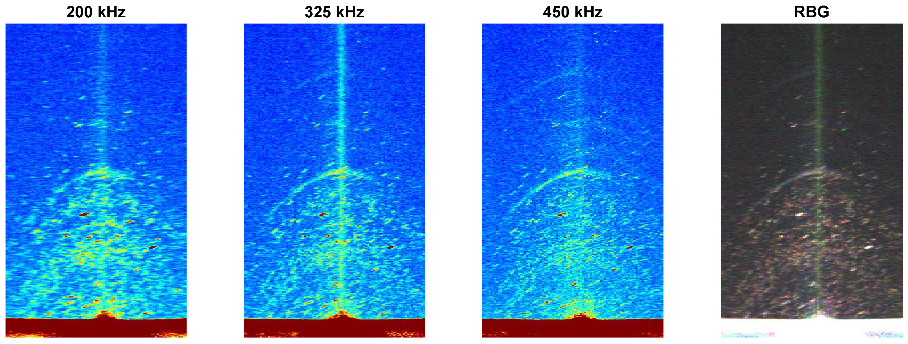
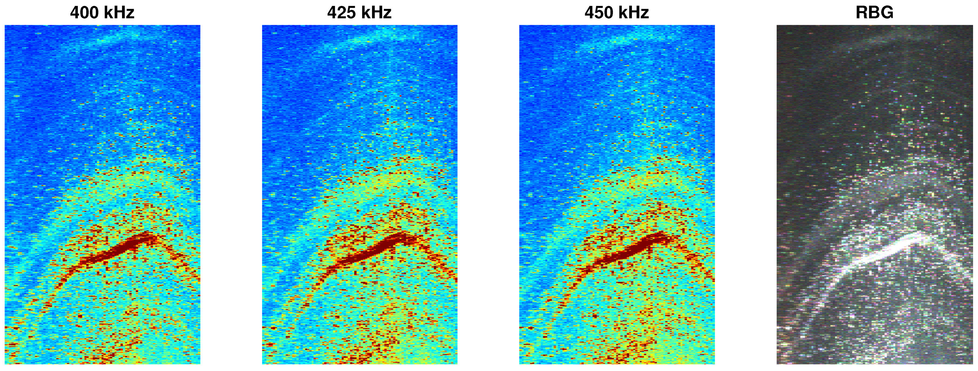
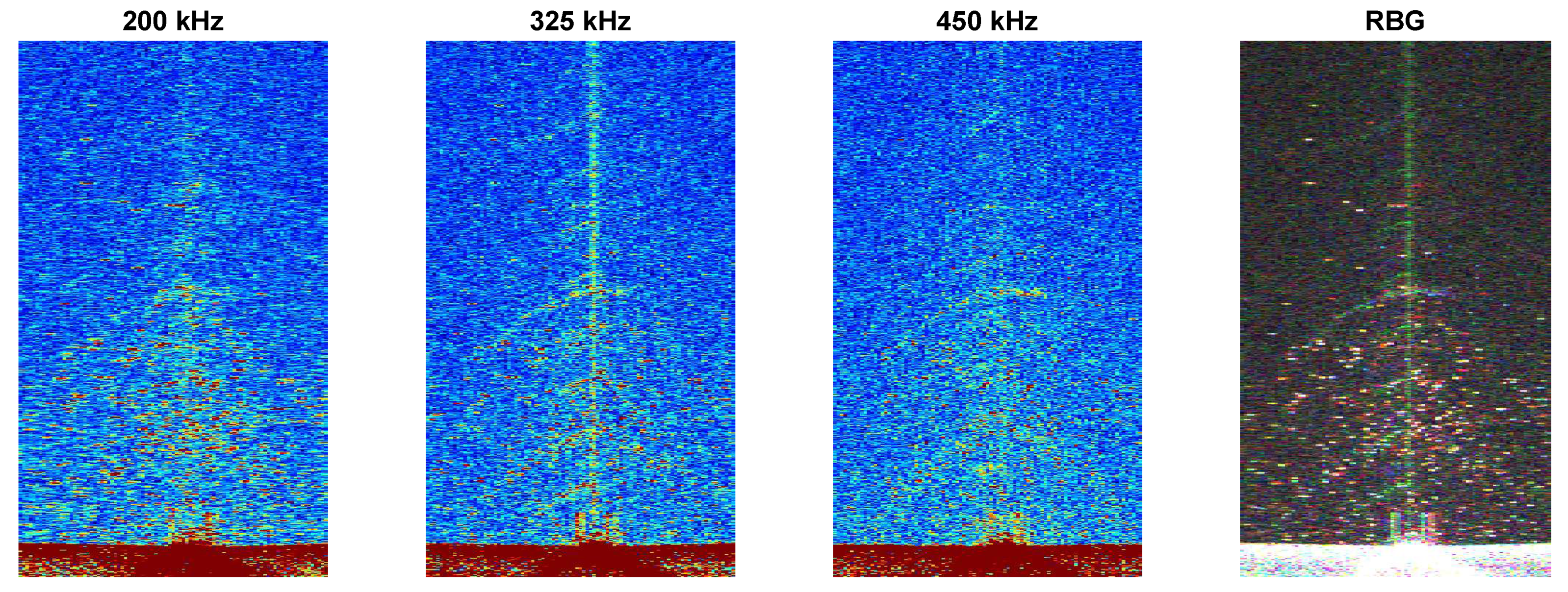
3.2.3. Observations Based on MultifrequencyRecords

To examine the differences in the water mass boundaries reflections for signals at different frequencies, we utilize the Mobile River data set, characterized by the largest range of frequencies: from 200 to 450 kHz. Figure 14 presents the visualization of water column data from three consecutive pings, transmitted every 0.0484 s, with the portion presenting the reflections from the water mass boundaries in the nadir zone enlarged.

The reflections from approximately horizontal features are distinct, with the visualization of higher frequencies (325 kHz and 450 kHz) distinguishing between individual reflections, although the analysis is impeded by the noisiness of the water column data in the analyzed range of amplitude values. Classical noise reduction techniques, derived from image processing, lead to the suppression of the weak signals reflected from the water mass boundaries. In [42], the authors suggest computing the time average of recorded pings along the track of the vessel to visualize the presence of an anomalous layer of interest. A similar approach has been tested here for noise reduction purposes. This technique was argued to reduce the random noise on images in [43], as the summation of random signals leads to its suppression, maintaining the existing signals, even if they are at or even below the level of noise. Figure 15 presents the result of summing 10 consecutive pings of a given frequency. Because the data were recorded in the multifrequency mode, where the frequencies interchange, the time period between two pings of the same frequency was equal to $0.0484\times 3=0.145$ s. Averaging 10 pings of the same frequency means in fact a spatial and temporal averaging of a time of 1.4 s. This distorts the information about the true shapes and movement parameters of detected boundaries, but if we can accept down-sampling to around 1.4 s of the ping period, some useful observations can be made based on this visualization.

The reflections are visible on all the records, although the highest frequency shows the clearest shape of the reflections. The weaker echoes in the upper parts of the images can be observed at the higher frequencies. They are not clearly distinguishable at 200 kHz, although the overall differences in the images are almost negligible.

The use of frequencies in the range of 400 to 450 kHz in multispectral mode for the datasets Old Channel A and Old Channel B results in almost no difference between the adjacent pings (Figure 16).

In order to illustrate the statement that the difference in frequencies from within the range used in the records has a minor impact on the data in terms of water column boundary detection, pseudo-RGB images have been created for all the generated images. The lowest frequency has been treated as the red channel, the middle frequency as the green channel and the highest frequency as the blue channel. The results are presented in Figure 14, Figure 15 and Figure 16 as the rightmost subfigures. None of the colors dominates here, and the white color showing strong reflections indicates the high contributions of the signals of all frequencies.

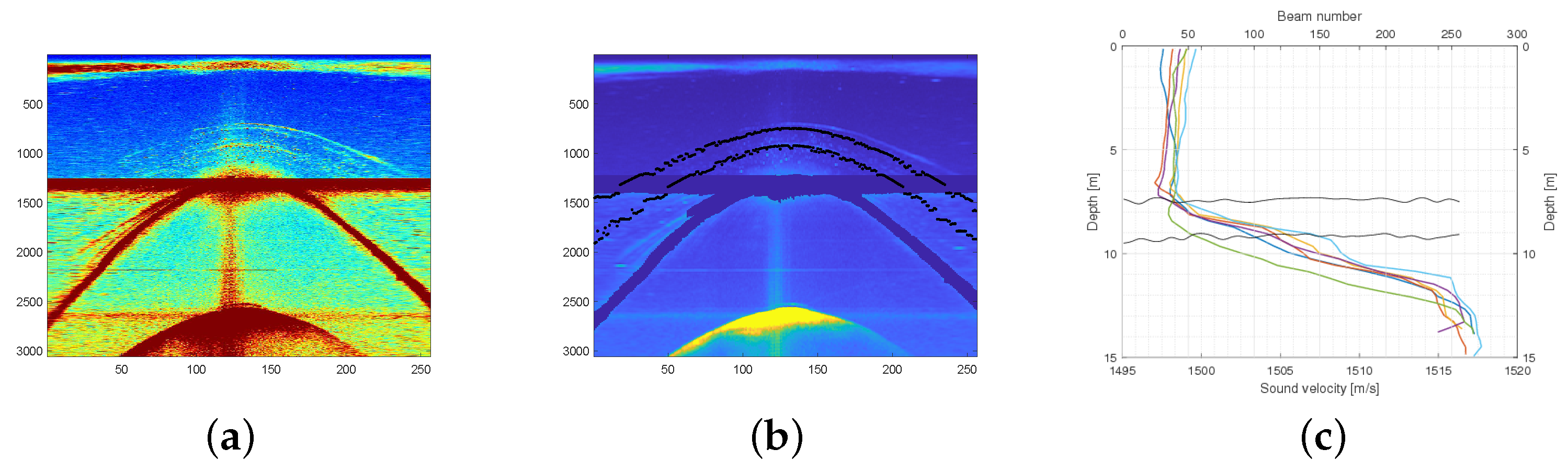
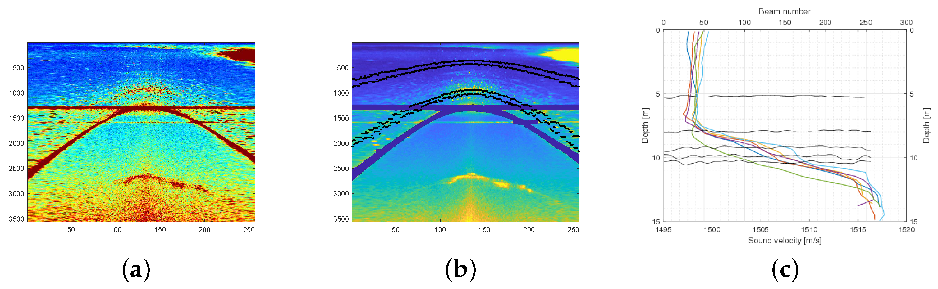
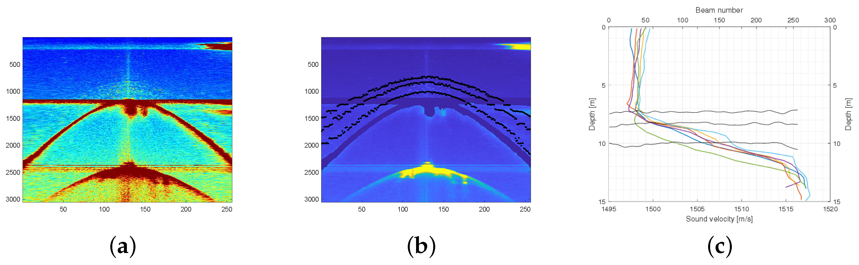
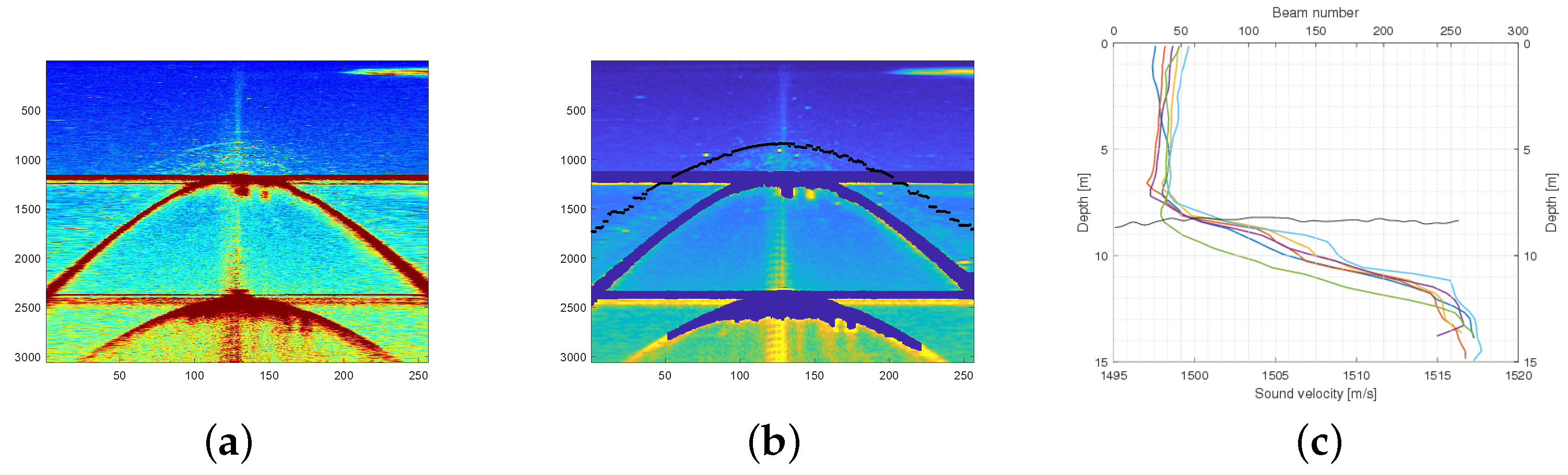
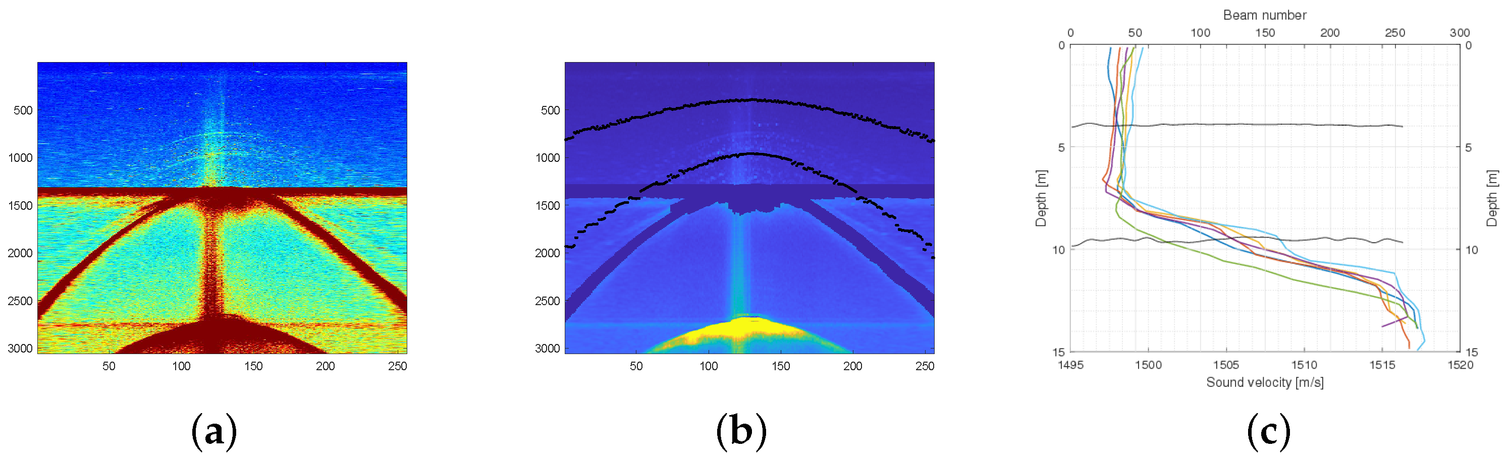
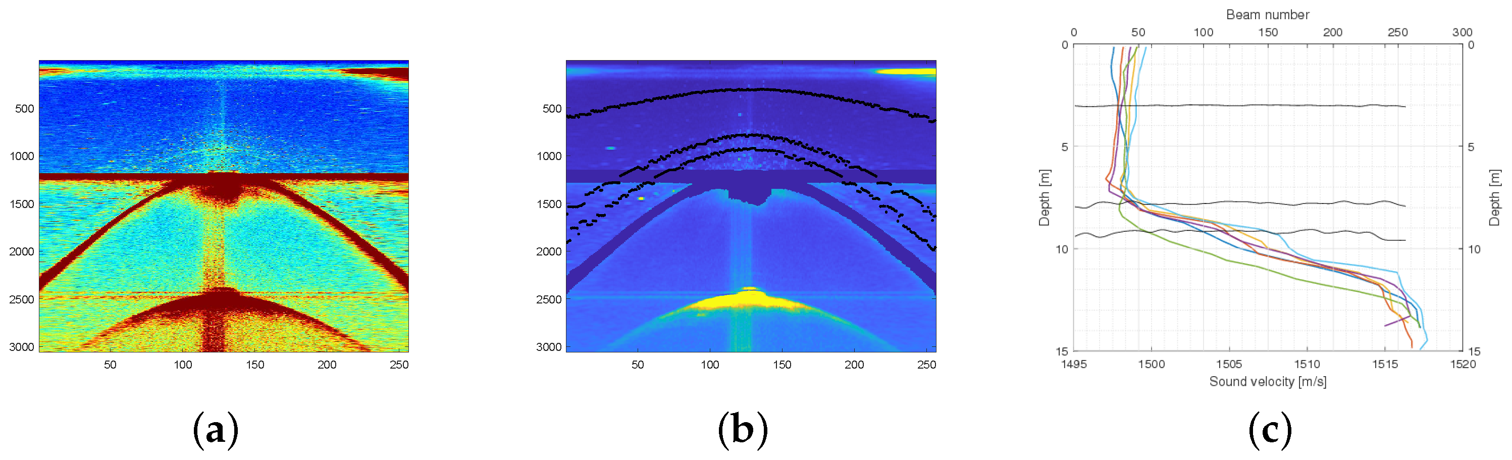
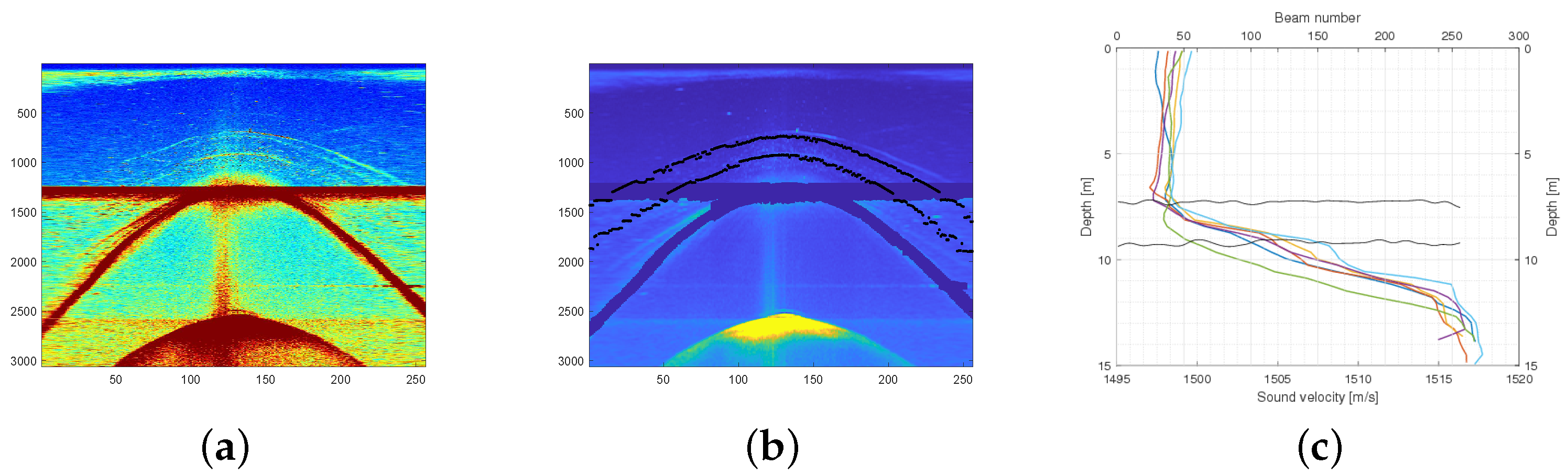
3.2.4. Automatic Detection of the Acoustic Reflection from Water Mass Boundaries in the Water ColumnData

The automatic detection of water mass layer boundaries can provide the desired information about these oceanographic phenomena in a fast and efficient manner, reducing the need to deal with large data sets each time, by providing the extraction of only the required information.

The following steps describe the proposed automated detection method for the water mass boundary reflection based on the image processing technique. The numbers of the steps refer to the scheme presented in Figure 17.

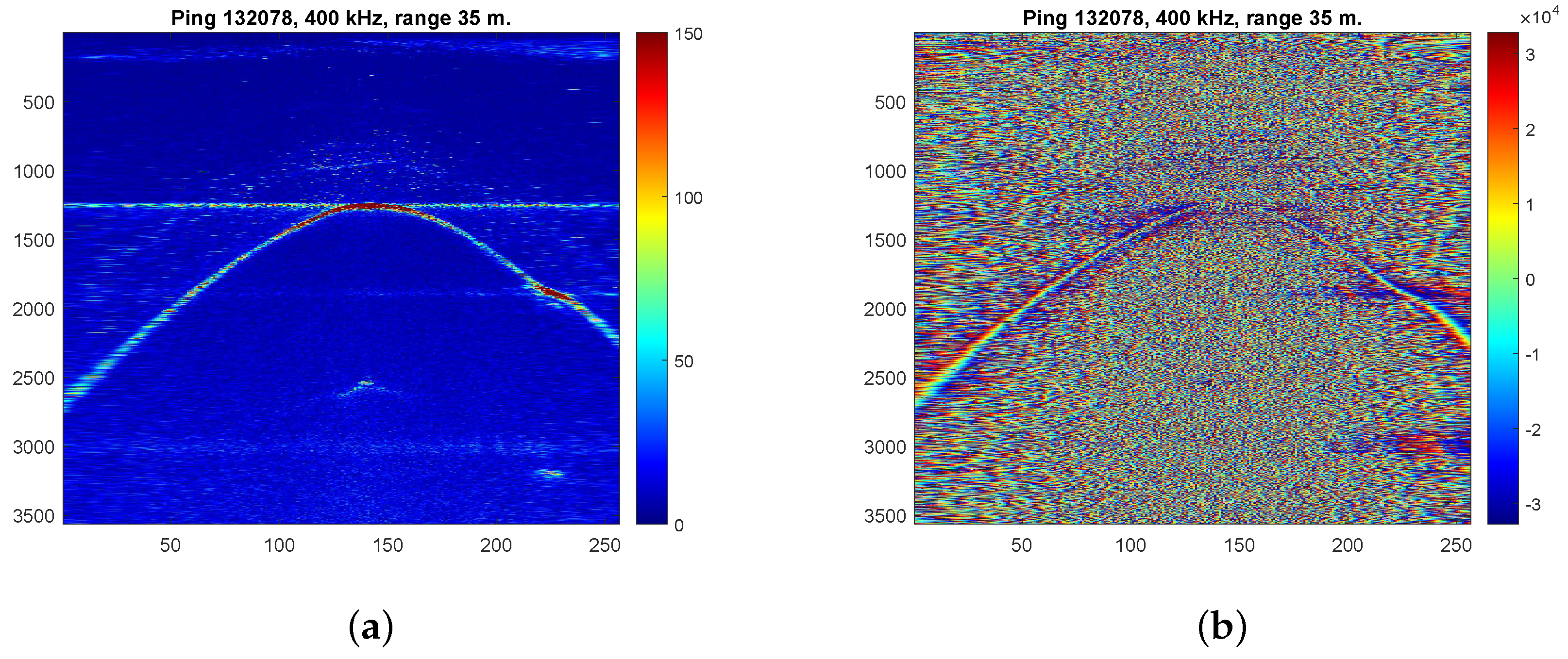
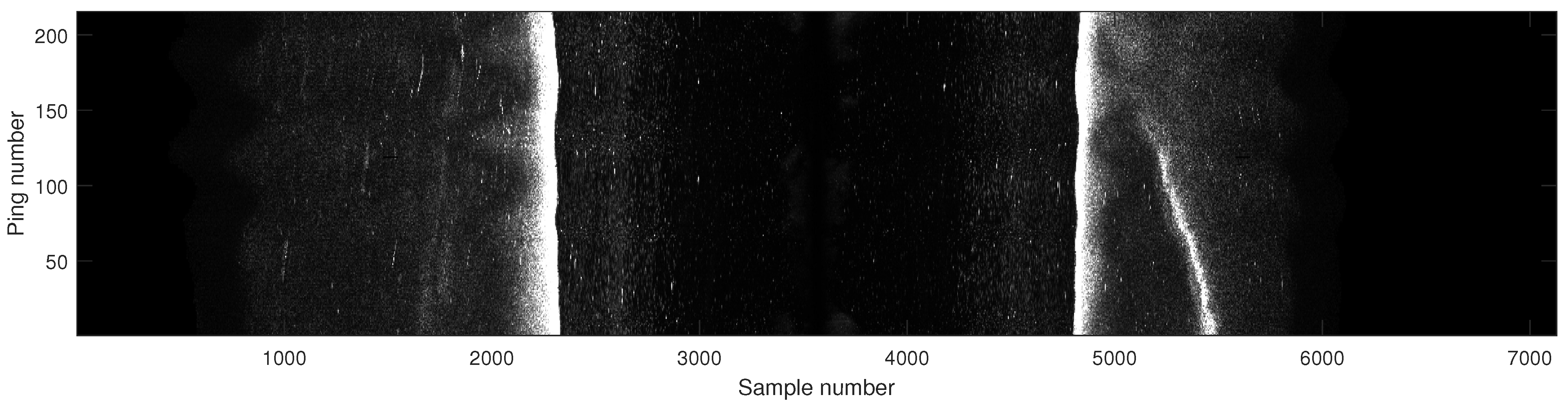
• Presenting the whole ping as a matrix of values representing the samples of all the beams: This is done for a series of a number of consecutive pings. This step is a preparatory stage, with the data simply treated as an image, allowing further processing by image processing techniques.
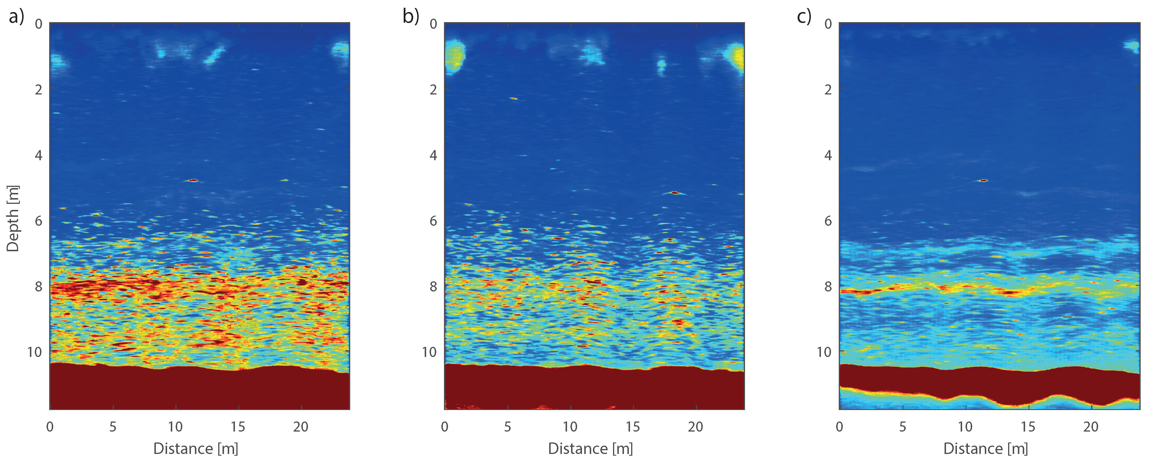
• De-noising by summing a number of consecutive pings: At the amplitude range referring to weak targets, the noise level makes the image difficult to process using the basic objects or edge detection methods. As proposed in Section 3.2.3, one of the possible methods of image de-noising, in case of a series of similar images presenting a similar scene, is the simple summation of a number of images. In the examples presented above, nine images were summed. It should be highlighted that this kind of mathematical operation means the averaging of data in time and space because we are dealing with the record from a moving sensor. However, if we realize that with the ping period of 0.055 s (in case of the Old Channel A data set), we average signals from 0.45 s of recordings, and if we consider the fact that the aim of this analysis is to reveal the information about the presence and characteristics of water mass boundaries and internal waves in our observations, this down-sampling seems to be acceptable.
• Smoothing: The Savitzky–Golay finite impulse response (FIR) smoothing filter with a polynomial order of 2 and frame length of 51 was applied to series of values from each beam independently, reducing the noise still remaining after the previous step.
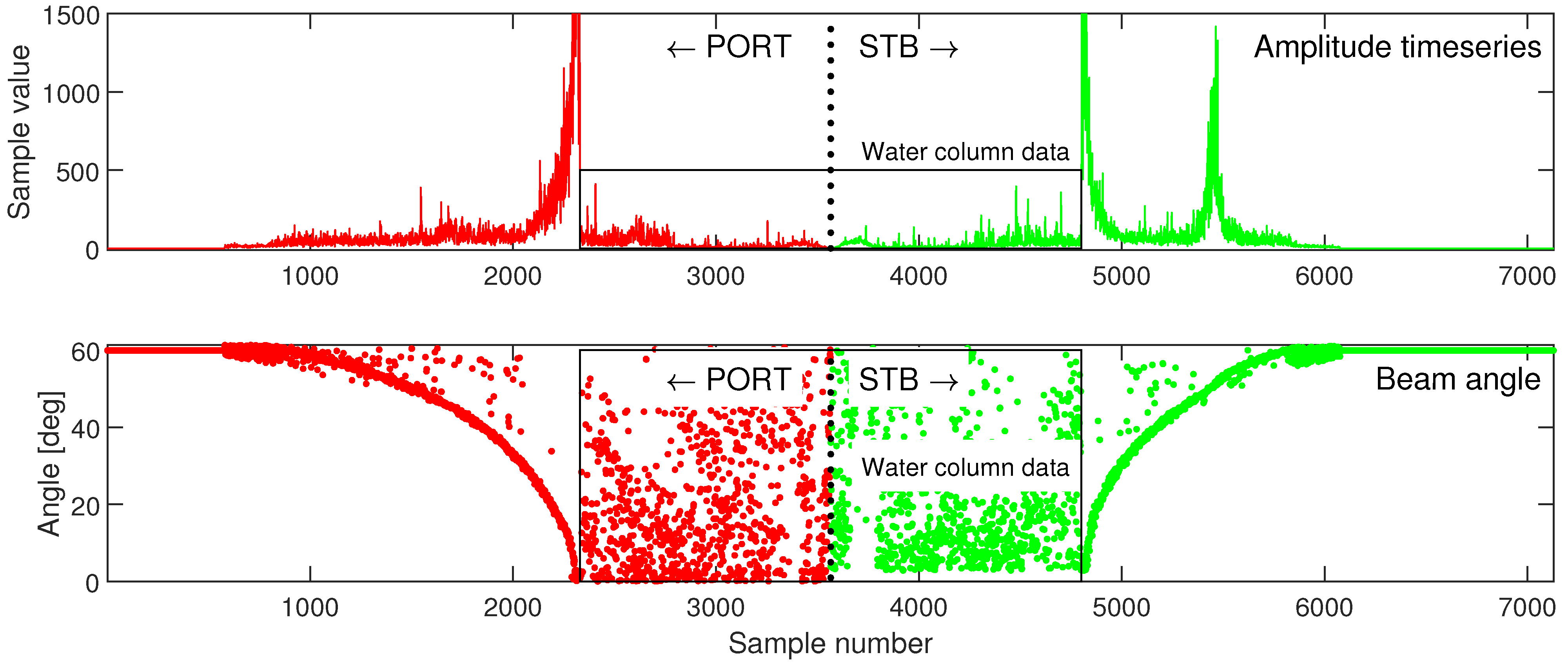
• Exclusion of the seabed and sidelobe areas from further analysis: High-magnitude values of samples corresponding to the main reflection from the seabed and the effect of sidelobes affect the operations performed on the areas of interest in the water column and outside the sidelobe. A large difference between those values and the “background” allows the exclusion of these areas easily by simple thresholding and by setting those samples to 0. The strong reflections from the seabed or solid objects in the water column are characteristic of a water column image and and are always present when a multibeam echosounder maps the seabed. Extracting these strong reflections allows for the further processing of the remaining data, which contains useful information for water column analysis.
• Contrast enhancement: This is done by the saturation of the bottom 1% and the top 1% of all pixel values. The embedded Matlab function imadjust was used for this purpose and appeared to be sufficient for the proposed method.
• Detection of the features approximately parallel to the sea surface by a summation of the values inside a moving sinusoidal mask: Reflections from the water mass boundaries might be too weak to appear in each beam, although the sinusoidal shape visible on the beam vs. time plot can be revealed. Those features will be then characterized by the higher values of samples in total along the line parallel to the sea surface, within some range of the possible fluctuations. As described in the visualizations above, this refers to the sinusoidal shape of the reflections; thus, moving sinusoidal masks are created to count the total values within it. The parameters of the sinusoidal mask boundaries and its width are dependent on the depth (sample number) and beam width for each summation. For each image, a series of sums is then created.
• Detection of peak sums: The peak in the series of calculated sums indicates the values higher than the surrounding background, creating a close-to-sinusoidal shape through all the beams.
• Detection of the strongest echos within each beam inside the moving masks chosen in the previous step: This results in the water mass boundaries being indicated as a series of points, similar to the seabed indication, although more than one is allowed for each ping.

The scheme of all the steps described above is presented in Figure 17:

Figure 17. The scheme of the steps of automatic water mass boundary detection based on image processing techniques.

Figure 17. The scheme of the steps of automatic water mass boundary detection based on image processing techniques.

4. Results

The records from four data sets have been subjected to all the steps of the proposed image processing algorithm. The figures below presents the results from all data sets. The original image and the processed image with the strongest reflections have been presented for each dataset. The chosen points during computation are given as the number of samples through each beam. With the angle information for each beam, the receiving range of the echosounder and the total number of samples, the selected sample number can be translated into the depth of this reflection. The results are presented in the rightmost plot for each of the presented cases. Black lines indicate the detected water mass boundaries for a particular series of pings (upper axis). Additionally, the measured sound speed profiles have been plotted using the same depth axis for comparison with the received boundaries depths.

Reference to the along-track cross-sections from Figure 7, Figure 8, Figure 9 and Figure 10 is very useful when analyzing the above results. The cross-sections depict the overall strength of the water column feature reflections or the presence of interference.

The examples of automated detection analysis from the Old Channel B data set are presented in Figure 18 and Figure 19. This dataset was recorded first, immediately before taking SVP cast 1, in close vicinity of this survey line (Figure 1). Easily recognizable sinusoidal reflections are clearly visible, and they have been picked up by the proposed method. The upper boundary detected here refers to the depth at which the sound speed rapidly starts to increase. A lower detection can be connected with a depth of around 9 to 10 m, where SVP casts indicate inconsistencies between measured sound velocity profiles.

The depths at which sound speeds show increasing rate inconsistencies have been picked up by the proposed algorithm in the images generated from the Old Chanel A data set (lower boundaries in Figure 20 and Figure 21). The upper boundary coincides with the depth at which the discrepancies between sound speeds, caused mostly by the measured temperature differences, start to disappear.

Similar results have been observed in the Mobile River data set (Figure 22 and Figure 23), although in most cases the algorithm was not able to pick up the weaker reflections from the upper part of the water column.

The results from Mobile Mouth (Figure 24 and Figure 25) are comparable to Old Channel A, while those survey lines were geographically close to each other and to the measurements in the area of SVP casts 2 to 5.

5. Discussion

The following observation can be made based on the conducted analysis and the observation of the algorithm results:

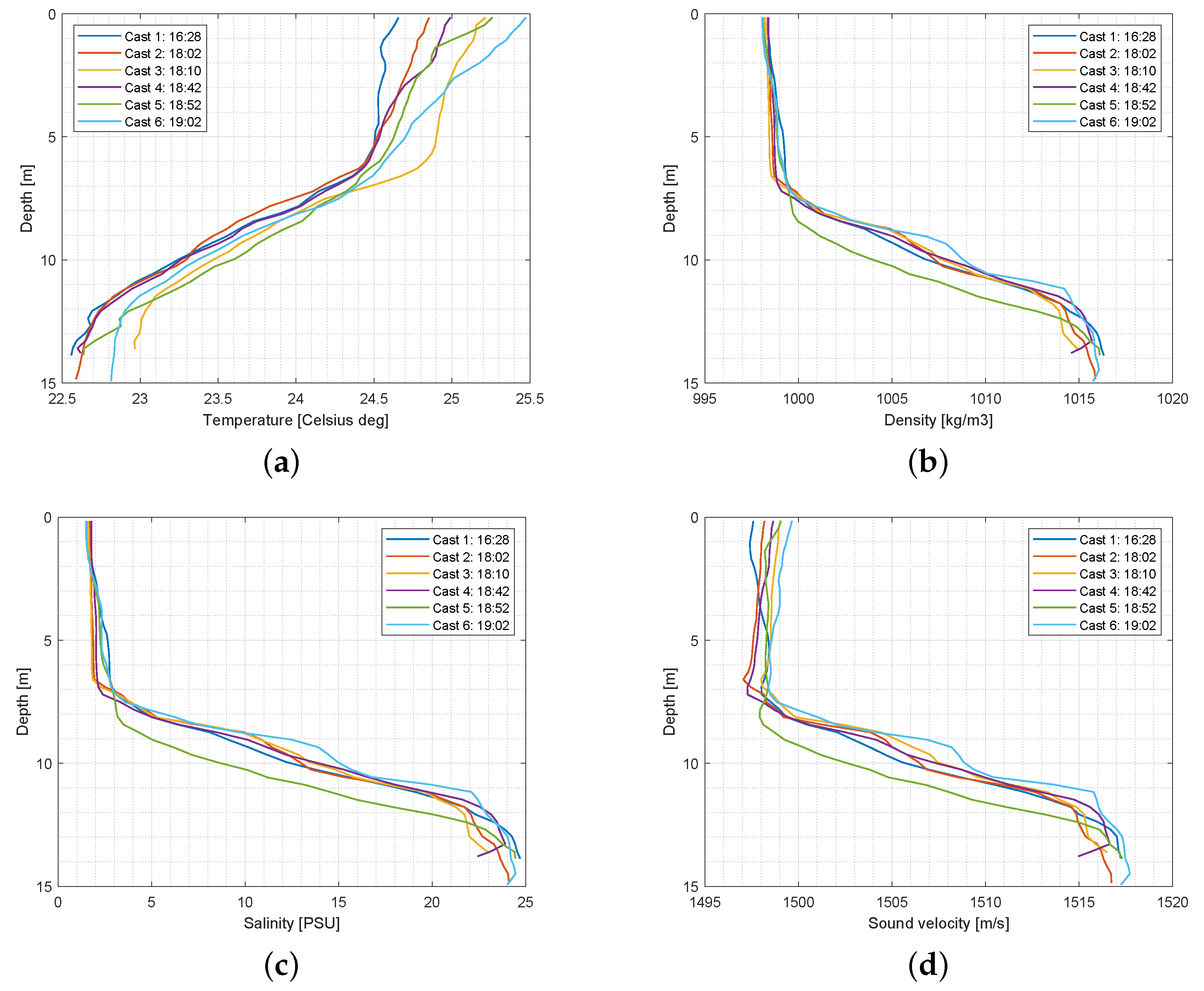
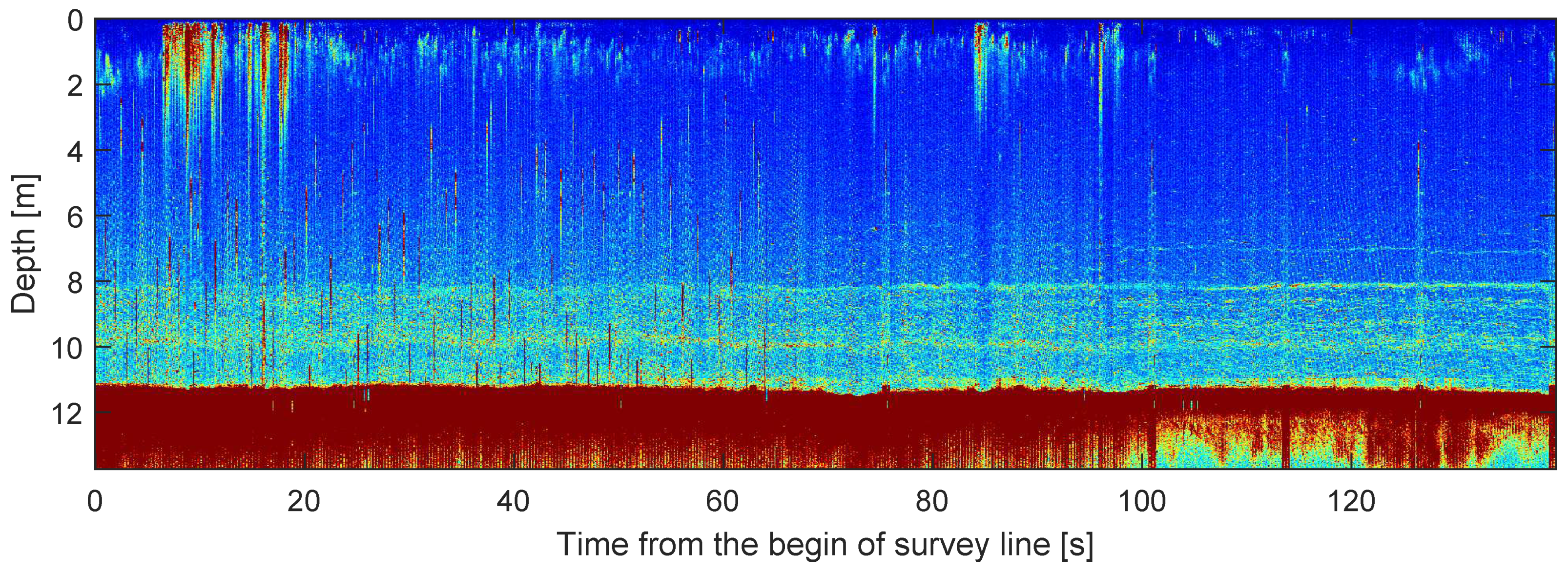
• It is possible to detect the depth of the rapid change of water properties at a particular moment of time, which can be used to update a currently used sound speed profile.
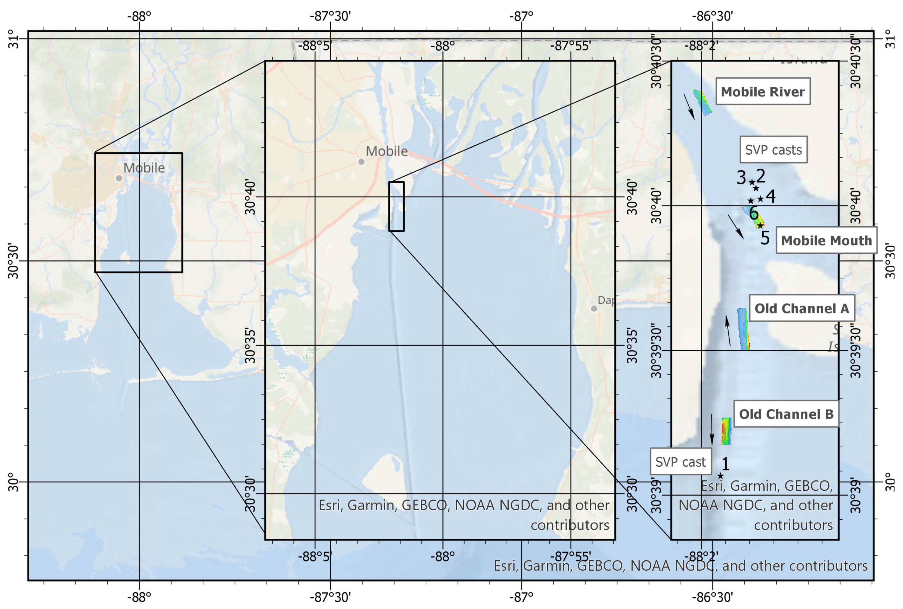
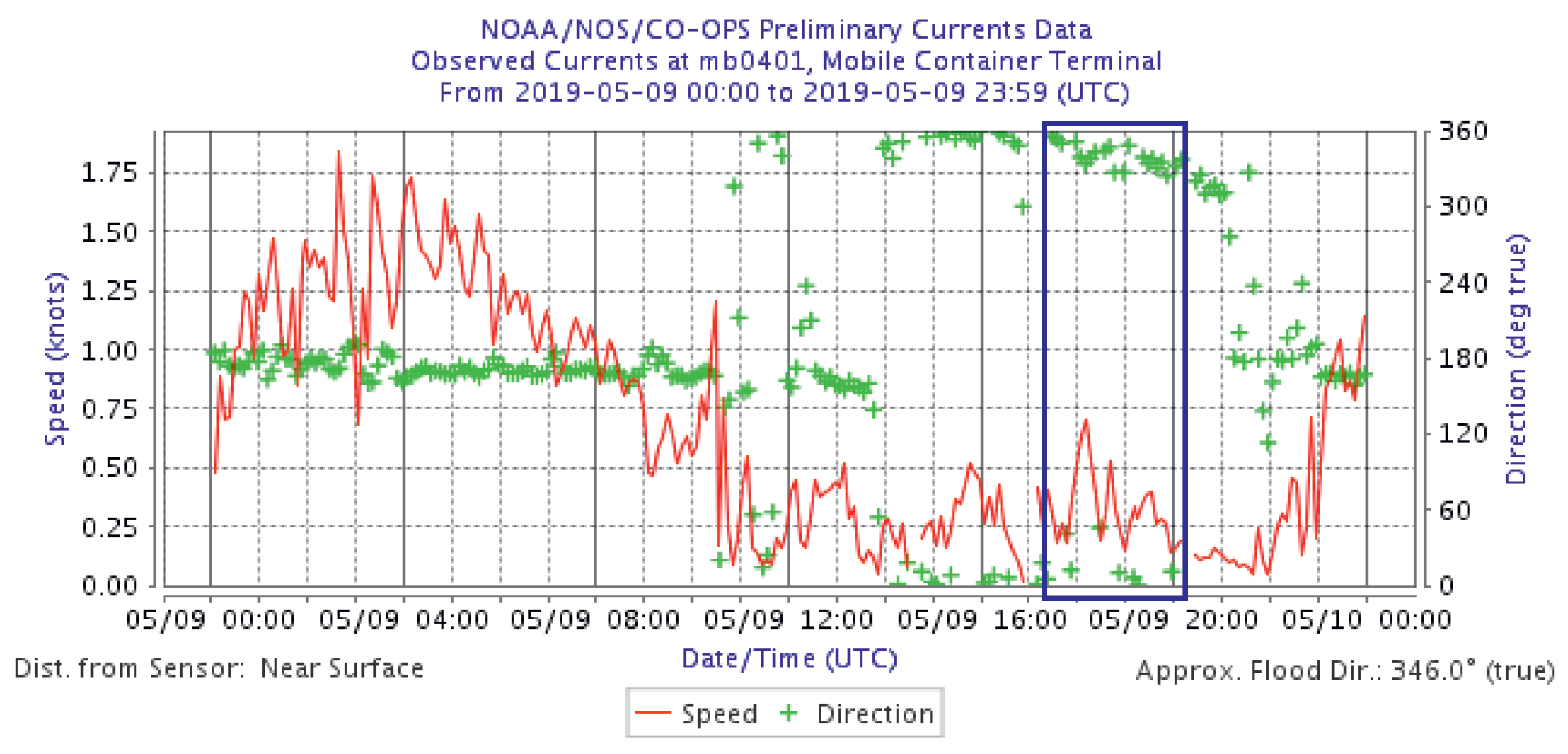
• The cross-sections are generated based on images presenting the acoustic responses of the seabed and water column, relative to the transducer. To determine the existence and the exact properties of internal waves, the vessel attitude, speed, and survey line shape must be taken into account. This is clearly visible on the records from Old Channel B and Old Channel A. Those lines both ran along the dredged shipping channel, but the first one (B) was recorded while running against the current of an incoming tide, while the second (A) ran with it. The period of the apparent sinusoidal-like shape visible in the cross-sections differs in these images, which may be caused by the sampling parameters of a moving vessel.
• Similar observations about the depth of the reflections from the strongest water mass boundaries can be made based on TruePix™ data, which are easy to process and require much less storage space.
• It was noticed that useful water column data are observed beyond the minimum slant range radius, which stands in contrast to the common routine of working only with water column data within the radius of the minimum slant range (e.g., [42]), recognizable by the sidelobes effect.

The acoustic responses of all the beams of the multibeam echosounder have been converted into image data and analyzed using the proposed automatic detection method, which resulted in the following observations:

• Similar to the along-track cross-sections, the results are based here on the image data. To obtain the exact depths of the reflections, vessel attitude must be taken into account.
• The proposed method takes into account the whole swath of all MBES beams. This results in providing across-track cross-sections of the water column structure, showing the major boundaries between the various water masses and their differing properties.
• The proposed method allows the use of the detected boundary depth for each beam separately, increasing the overall accuracy of the determined depth.
• It has been observed and presented in the examples that the number of detected boundaries may vary between images. Some of the reflections were overall too weak to be picked up from the background, with some noise left after de-noising routines.
• The detected boundaries between water masses of varying properties can be compared with the sound speed profiles collected at two locations in the survey area. The ranges of detected boundary depths correspond with the indications of sound speed profiles, although exact values differ, and they refer to the particular time that input MBES data were collected. This reflects the movement of the boundaries caused by the mechanisms described in the introductory sections.

The proposed method can be used to automatically detect the boundaries between water masses with varying acoustic impedances from the multibeam water column data. Running the proposed method on the data collected by the MBES over a particular time on a survey line can lead to the construction of the water column structure model. Adding the spatial data of the vessel movement can bring these data into the three-dimensional space, presenting a dynamic water column structure. The incorporation of the detected depth of rapid water mass parameter change into the seabed depth determination algorithm can improve its accuracy, and this can be done separately for each beam, taking into account the across-track variability of the water column, which changes over time. Additionally, while using the existing commercial software solutions, the knowledge about the range of the boundary oscillation can be used as an additional factor in the error budget.

Large-scale internal waves are evident on the synthetic aperture radar (SAR) images collected from satellites [44,45,46]. This is a preferred method for studying the environmental relationships over large areas, although the resolution of the SAR data, varying from 6 to 30 m (for the ERS-1 and ERS-2 satellites launched by European Space Agency [44]), disqualifies these kinds of methods for local applications, such as studying particular estuaries, river inlets, and smaller basins. There have been successful attempts to study the characteristics of water mass stratification and its movements due to internal wave mechanisms using seismic methods. The authors of [47] present the observation of the temporal changes of an interface between layers in the Panama Basin, based on high-resolution seismic reflection imaging. The authors in [48] found that, using multichannel seismic reflection data acquired from the Tyrrhenian Sea, they could clearly delineate the finer structure in the thermohaline; this was verified with CTD probes. The authors of [49] went further and used seismic reflection imaging to provide quantitative information regarding internal waves in the Norwegian Sea. Through their analysis, the authors demonstrated that seismic oceanography can quantify the internal wave field over large areas and can even provide estimates of the energy within the internal waves. However, the use of seismic techniques requires expensive towed arrays, in comparison to the method utilized above using MBES water column data.

Multibeam echosounder water column data have been widely analyzed in the literature in terms of gas seepage detection, fish school identification, and searching for objects suspended in the water column. Trials with water mass boundary detection in real time, to deal with movement between SVP casts due to the internal wave mechanism, are relatively new. Similar works has been conducted using single-beam echosounders, such as that described in [50]. The single-beam echosounder profile of large internal wave packets observed in Tarif Narrow in Gibraltar is presented in [50]. Internal wave imaging by a single-beam echosounder is also presented in [51]. Multibeam data, in contrast to single-beam data, allow the addition of the second dimension to the derived model of the water column.

6. Conclusions

It was assumed that, to include the impact of internal waves in hydrographic measurements, the current boundaries between water masses with different properties should be determined at the time of measurement, knowing that boundaries change both spatially and over time. It was proposed that this boundary recognition could be conducted by the analysis of water column data, treating the samples of all the beams as an image that is analyzable by using image processing techniques. Along-track cross-sections through all the pings of a particular survey lines have been generated.

Using a multibeam echosounder allows us to look not only along the track of the survey line, which is also possible using the single-beam echosounder, but also to generate the across-track cross-sections for each ping or a series of pings. One must be aware that the features detected here are in fact not well defined (it is not a solid object located precisely in the space). The only factor that we are trying to detect is the location of the change of water properties, which causes a slightly different behavior of the sound wave. The lack of ground truth data is the factor that makes the quantification of the results, understood as a mathematical comparison with the known reference, impossible to conduct. After the standard hydrographic survey, the only reference data about the water properties are the discrete sound speed profiles. To overcome this, an interesting option might be to survey a particular spot with a stationary mounted multibeam echosounder while measuring the water mass parameters, preferably simultaneously, at different depths through the water column. This methodology can be used in further research.

References

1. Medwin, H. Sounds in the Sea: From Ocean Acoustics to Acoustical Oceanography; Cambridge University Press: Campbridge, UK, 2005. [Google Scholar]
2. Hamilton, T.; Beaudoin, J. Modeling the Effect of Oceanic Internal Waves on the Accuracy of Multibeam Echosounders. Int. Hydrogr. Rev. 2010, 4, 55–65. [Google Scholar]
3. Helfrich, K.R.; Melville, W.K. Long nonlinear internal waves. Annu. Rev. Fluid Mech. 2006, 38, 395–425. [Google Scholar] [CrossRef]
4. Santos-Ferreira, A.M.; Da Silva, J.C.B.; Magalhaes, J.M. SAR Mode Altimetry Observations of Internal Solitary Waves in the Tropical Ocean Part 1: Case Studies. Remote Sens 2018, 10, 644. [Google Scholar] [CrossRef] [Green Version]
5. Liang, J.; Li, X.-M.; Sha, J.; Jia, T.; Ren, Y. The lifecycle of nonlinear internal waves in the northwestern South China Sea. J. Phys. Ocean. 2019, 49, 2133–2145. [Google Scholar] [CrossRef]
6. Gao, Q.; Dong, D.; Yang, X.; Husi, L.; Shang, H. Himawari-8 Geostationary Satellite Observation of the Internal Solitary Waves in The South China Sea. Int. Arch. Photogramm. Remote. Sens. Spat. Inf. Sci. 2018, XLII, 7–10. [Google Scholar] [CrossRef] [Green Version]
7. LeBlond, P.H.; Mysak, L.A. Waves in the Ocean; Elsevier: Amsterdam, The Netherlands, 1978. [Google Scholar]
8. Apel, J.R. A New Analytical Model for Internal Solitons in the Ocean. J. Phys. Oceanogr. 2003, 33, 2247–2269. [Google Scholar] [CrossRef]
9. Badiey, M.; Mu, Y.; Lynch, J.F.; Tang, X.; Apel, J.R.; Wolf, S. Azimuthal and temporal dependence of sound propagation due to shallow water internal waves. IEEE J. Ocean. Eng. 2002, 27, 117–129. [Google Scholar] [CrossRef]
10. Li, L.; Pawlowicz, R.; Wang, C. Seasonal variability and generation mechanisms of nonlinear internal waves in the Strait of Georgia. J. Geophys. Res. Ocean. 2018, 123, 5706–5726. [Google Scholar] [CrossRef]
11. Wang, C.; Wang, X.; Da Silva, J.C.B. Studies of Internal Waves in the Strait of Georgia Based on Remote Sensing Images. Remote Sens. 2019, 11, 96. [Google Scholar] [CrossRef] [Green Version]
12. Magalhaes, J.M.; Da Silva, J.C.B. Internal Solitary Waves in the Andaman Sea: New Insights from SAR Imagery. Remote Sens. 2018, 10, 861. [Google Scholar] [CrossRef] [Green Version]
13. Lamb, K.G. Internal Wave Breaking and Dissipation Mechanisms on the Continental Slope/Shelf. Annu. Rev. Fluid Mech. 2014, 46, 231–254. [Google Scholar] [CrossRef]
14. Sutherland, B. Internal Gravity Waves; Cambridge University Press: Cambridge, UK, 2010. [Google Scholar] [CrossRef]
15. Klusek, Z. Conditions for Sound Propagation in the Southern Baltic. Ph.D. Thesis, Polish Academy of Science, Oceanology Institute, Warsaw, Poland, 1999; pp. 30–31. [Google Scholar]
16. Shengxuan, L.; Xiuyun, C. The Effect of Oceanic Internal Waves on Multibeam Echosounding. Hydrogr. Surv. Charting 2012, 32, 27–29. [Google Scholar]
17. Hughes Clarke, J.E. Coherent refraction “noise” in multibeam data due to oceanographic turbulence. In Proceedings of the US Hydrographic Conference, Galveston, TX, USA, 25 July 2017. 18p. [Google Scholar]
18. Hughes Clarke, J.E. The Impact of Acoustic Imaging Geometry on the Fidelity of Seabed Bathymetric Models. Geosciences 2018, 8, 109. [Google Scholar] [CrossRef] [Green Version]
19. Vilming, S. The Development of the Multibeam Echosounder: A Historical Account. J. Acoust. Soc. Am. 1998, 103, 5. [Google Scholar] [CrossRef]
20. Lurton, X. An Introduction to Underwater Acoustics; Springer: Berlin/Heidelberg, Germany, 2002. [Google Scholar]
21. Fundamentals of Naval Weapons Systems, Weapons and Systems Engineering Deptartment, US Naval Academy. Available online: https://fas.org/man/dod-101/navy/docs/fun/index.html (accessed on 24 February 2020).
22. Urick, R.J. Principles of Underwater Sound; McGraw-Hill: New York, NY, USA, 1983. [Google Scholar]
23. Blomberg, A.E.A.; Weber, T.C.; Austeng, A. Improved Visualization of Hydroacoustic Plumes Using the Split-Beam Aperture Coherence. Sensors 2018, 18, 7. [Google Scholar] [CrossRef] [Green Version]
24. Colbo, K.; Ross, T.; Brown, C.; Weber, T.C. A review of oceanographic applications of water column data from multibeam echosounders. Estuarine Coast. Shelf Sci. 2014, 145, 41–56. [Google Scholar] [CrossRef]
25. Caruthers, J.W. Fundamentals of Marine Acoustics; Elsevier: Amsterdam, The Netherlands, 1977; p. 64. [Google Scholar]
26. Hughes Clarke, J.E. Applications of multibeam water column imaging for hydrographic survey. Hydrogr. J. 2006, 120, 3. [Google Scholar]
27. Noble, M.A.; Schroeder, W.W.; Wiseman, W.J., Jr.; Ryan, H.F.; Gelfenbaum, G. Subtidal circulation patterns in a shallow, highly stratified estuary: Mobile Bay, Alabama. J. Geophys. Res. 1996, 101, 689–703. [Google Scholar] [CrossRef]
28. Schroeder, W.W.; Lysinger, W.R. Hydrography and Circulation of Mobile Bay. In Symposium on the Natural Resources of the Mobile Bay Estuary; Loyacano, H.A., Smith, J.P., Eds.; U.S. Army Corps of Engineers: Washington, DC, USA, 1979; pp. 75–94. [Google Scholar]
29. Wiseman, W.J., Jr.; Schroeder, W.W.; Dinnel, S.P. Shelf-Estuarine Water Exchanges between the Gulf of Mexico and Mobile Bay, Alabama. Am. Fish. Soc. Symp. 1988, 3, 1–8. [Google Scholar]
30. Drymon, J.M.; Ajemian, M.J.; Powers, S.P. Distribution and dynamic habitat use of young bull sharks Carcharhinus leucas in a highly stratified northern Gulf of Mexico estuary. PLoS ONE 2014, 9, e97124. [Google Scholar] [CrossRef]
31. Ryan, J.J.; Goodell, H.G. Marine Geology and Estuarine History of Mobile Bay, Alabama Part 1. Contemporary Sediments. Environ. Framew. Coast. Plain Estuaries 1972, 18. [Google Scholar] [CrossRef]
32. Cambazoglu, M.K.; Soto, I.M.; Howden, S.D.; Dzwonkowski, B.; Fitzpatrick, P.J.; Arnone, R.A.; Jacobs, G.A.; Lau, Y.H. Inflow of shelf waters into the Mississippi Sound and Mobile Bay estuaries in October 2015. J. Appl. Rem. Sens. 2017, 11, 032410. [Google Scholar] [CrossRef] [Green Version]
33. NOAA Tides & Currents, Mobile Container Terminal (mb0401). Available online: https://tidesandcurrents.noaa.gov (accessed on 2 March 2020).
34. SONIC. 2026/2024/2022 Broadband Multibeam Echosounders, Operation Manual V6.3, Revision 003, 28 February 2019, Part No. 96000001. Documentation assocciated with the data, obtained from the R2Sonic company. unpublished.
35. Gaida, T.C.; Tengku Ali, T.A.; Snellen, M.; Amiri-Simkooei, A.; Van Dijk, T.A.G.P.; Simons, D.G. A Multispectral Bayesian Classification Method for Increased Acoustic Discrimination of Seabed Sediments Using Multi-Frequency Multibeam Backscatter Data. Geosciences 2018, 8, 455. [Google Scholar] [CrossRef] [Green Version]
36. Brown, C.J.; Beaudoin, J.; Brissette, M.; Gazzola, V. Multispectral Multibeam Echo Sounder Backscatter as a Tool for Improved Seafloor Characterization. Geosciences 2019, 9, 126. [Google Scholar] [CrossRef] [Green Version]
37. QPS. How-to Methods Used to Acquire Sonar Imagery. Available online: https://confluence.qps.nl/qinsy/8.0/en/how-to-methods-used-to-acquire-sonar-imagery-52101176.html (accessed on 7 December 2019).
38. R2Sonic. 2019 MS Challenge Data and File Format Info, unpublished report by R2sonic. Documentation assocciated with the data, obtained from the R2Sonic company. unpublished.
39. Beaudoin, J.; Clarke, J.H.; Bartlett, J. Application of Surface Sound Speed Measurements in Post-processing for Multi-Sector Multibeam Echosounders. IHR 2004, 5, 3. [Google Scholar]
40. Cheynet, E. Pcolor in Polar Coordinates. MATLAB Central File Exchange. 2020. Available online: https://www.mathworks.com/%20matlabcentral/fileexchange/%2049040-pcolor-in-polar-coordinates.html (accessed on 26 February 2020).
41. Cordero Ros, J.M. Improved Sound Speed Control through Remotely Detecting Strong Changes in Thermocline. Master’s Theses, University of New Hampshire, Durham, NH, USA, 2018. Available online: https://scholars.unh.edu/thesis/1245 (accessed on 17 March 2020).
42. Church, I.; Lauren, Q.; Williamson, M. Multibeam Water Column Data Processing Techniques to Facilitate Scientific Bio-Acoustic Interpretation. Available online: http://www.omg.unb.ca/wordpress/papers/Church_USHydro_2017.pdf (accessed on 19 March 2020).
43. Stateczny, A.; Praczyk, T. Sztuczne Sieci Neuronowe w Rozpoznawaniu Obiektów Morskich [In Polish]; Gdanskie Towarzystwo Naukowe: Gdansk, Poland, 2002; ISBN 83-87359-68-2. [Google Scholar]
44. Hsu, M.K.; Liu, A.K.; Liu, C. A study of internal waves in the China Seas and Yellow Sea using SAR. Cont. Shelf Res. 2000, 20, 389–410. [Google Scholar] [CrossRef]
45. Kozlov, I.; Romanenkov, D.; Zimin, A.; Chapron, B. SAR observing large-scale nonlinear internal waves in the White Sea. Remote Sens. Environ. 2014, 147, 99–107. [Google Scholar] [CrossRef] [Green Version]
46. Li, X.; Clemente-Colon, P.; Friedman, K.S. Estimating oceanic mixed-layer depth from internal wave evolution observed from Radarsat-1 SAR. Johns Hopkins APL Tech. Dig. 2000, 21, 130–135. [Google Scholar]
47. Tang, Q.; Tong, V.; Hobbs, R.W.; Morales Maqueda, M.A. Detecting changes at the leading edge of an interface between oceanic water layers. Nat. Commun. 2019, 10, 4674. [Google Scholar] [CrossRef] [PubMed] [Green Version]
48. Buffett, G.G.; Krahmann, G.; Klaeschen, D.; Schroeder, K.; Sallares, V.; Papenberg, C.; Ranero, C.R.; Zitellini, N. Seismic oceanography in the Tyrrhenian Sea: Thermohaline staircases, eddies, and internal waves. J. Geophys. Res. Ocean. 2017, 122, 8503–8523. [Google Scholar] [CrossRef] [Green Version]
49. Holbrook, W.S.; Fer, I. Ocean internal wave spectra inferred from seismic reflection transects. Geophys. Res. Lett. 2005, 32. [Google Scholar] [CrossRef] [Green Version]
50. Apel, J.R. Oceanic Internal Waves and Solitons, An Atlas of Oceanic Internal Solitary Waves; Global Ocean Associates for Office of Naval Research, Global Ocean Associates: Silver Spring, MD, USA, 2002; pp. 1–40. [Google Scholar]
51. Gerkema, T.; Zimmerman, J.T.F. An Introduction to Internal Waves. Lecture Notes, Royal NIOZ, Texel 207, 2008. Available online: https://www.vliz.be/ (accessed on 21 February 2020).
Figure 1. The location map of four water column data sets, represented by the color–coded bathymetry hill–shades, collected at the mouth of the Mobile River, southern Alabama, United States. Stars indicate the locations of SVP casts. Black arrows indicate the general course of the vessel during data recording.
Energies 14 04774 g001
Figure 2. Surface current data recorded at the Mobile Container Terminal station (MB0401). Source: [33]. Time frame of the survey indicated by the blue rectangle.
Energies 14 04774 g002
Figure 3. Main parameters of the water mass, recorded in six casts taken in the survey area: (a) temperature; (b) seawater density; (c) salinity; (d) sound speed profiles.
Energies 14 04774 g003
Figure 4. The pseudo-color plots of 3564 samples for each of 256 beams for the one example ping. (a) Visualization of magnitude values; (b) phase values.
Energies 14 04774 g004
Figure 5. The wedge-shape plots of 3564 samples for each of the 256 beams for one example ping. (a) Visualization of magnitude values; (b) phase values.
Energies 14 04774 g005
Figure 6. Subset of the polar plot display of the acoustic intensities, with the characteristic elements of the receiving ping explained. Our own Matlab script has been used for data visualization. Explanations based on [26].
Energies 14 04774 g006
Figure 7. Along-track cross-section (average of 10 nadir beams) of water column data for the Old Channel B data set at three frequencies (400, 425, 450 kHz) recorded simultaneously using the multispectral mode.
Energies 14 04774 g007
Figure 8. Along-track cross-section (average of 10 nadir beams) of water column data for the Old Channel A data set at three frequencies (400, 425, 450 kHz) recorded simultaneously using the multispectral mode.
Energies 14 04774 g008
Figure 9. Along-track cross-section (average of 10 nadir beams) of water column data for the Mobile River data set at three frequencies (200, 325, 450 kHz) recorded simultaneously using the multispectral mode.
Energies 14 04774 g009
Figure 10. Along track cross-section (average of 10 nadir beams) of water column data for the Mobile Mouth data set at three frequencies (350, 400, 450 kHz) recorded simultaneously using the multispectral mode.
Energies 14 04774 g010
Figure 11. Visualization of amplitude time series information stored in TruePix™ files, creating an image similar to a side scan sonograph.
Energies 14 04774 g011
Figure 12. Amplitude and angle time series for the first ping of the Old Channel A record.
Energies 14 04774 g012
Figure 13. A visualization of TruePix™ data for an example of water column data for the port side (a) and starboard side (b), compared to the across-track section of R2S data (c).
Energies 14 04774 g013
Figure 14. Subsets of visualizations of three consecutive pings, each transmitted at a different frequency. The far-right image presents the pseudo-RGB compilation of the values of samples magnitudes from the three left images.
Energies 14 04774 g014
Figure 15. Subsets of visualizations of averaging 10 consecutive pings transmitted at one frequency for all the frequencies used in multispectral mode (here, 200, 325, and 450 kHz). The far-right image presents the pseudo-RGB compilation of the values of samples magnitudes from the three left images.
Energies 14 04774 g015
Figure 16. Subsets of visualizations of averaging 10 consecutive pings transmitted at one frequency, for all the frequencies used in multispectral mode (here, 400, 425, and 450 kHz). The far-right image presents the pseudo-RGB compilation of the values of sample magnitudes from the three left images. Data from Old Channel A dataset.
Energies 14 04774 g016
Figure 18. The results of automated water mass boundary detection from the Old Channel B dataset—example 1. (a) Original image, generated from a series of nine consecutive pings. (b) The result of the algorithm. (c) Detected boundaries plotted with the sound speed visualization for depth reference.
Energies 14 04774 g018
Figure 19. The results of automated water mass boundary detection from the Old Channel B dataset—example 2. (a) Original image, generated from a series of nien consecutive pings. (b) The result of the algorithm. (c) Detected boundaries plotted with the sound speed visualization for depth reference.
Energies 14 04774 g019
Figure 20. The results of automated water mass boundary detection from the Old Channel A dataset—example 1. (a) Original image, generated from a series of nine consecutive pings. (b) The result of the algorithm. (c) Detected boundaries plotted with the sound speed visualization for depth reference.
Energies 14 04774 g020
Figure 21. The results of automated water mass boundary detection from the Old Channel A dataset—example 2. (a) Original image, generated from a series of nine consecutive pings. (b) The result of the algorithm. (c) Detected boundaries plotted with the sound speed visualization for depth reference.
Energies 14 04774 g021
Figure 22. The results of automated water mass boundary detection from the Mobile River dataset—example 1. (a) Original image, generated from a series of nine consecutive pings. (b) The result of the algorithm. (c) Detected boundaries plotted with the sound speed visualization for depth reference.
Energies 14 04774 g022
Figure 23. The results of automated water mass boundary detection from the Mobile River dataset—example 1. (a) Original image, generated from a series of nine consecutive pings. (b) The result of the algorithm. (c) Detected boundaries plotted with the sound speed visualization for depth reference.
Energies 14 04774 g023
Figure 24. The results of automated water mass boundary detection from the Mobile Mouth dataset—example 1. (a) Original image, generated from a series of nine consecutive pings. (b) The result of the algorithm. (c) Detected boundaries plotted with the sound speed visualization for depth reference.
Energies 14 04774 g024
Figure 25. The results of automated water mass boundary detection from the Mobile Mouth dataset—example 1. (a) Original image, generated from a series of nine consecutive pings. (b) The result of the algorithm. (c) Detected boundaries plotted with the sound speed visualization for depth reference.
Energies 14 04774 g025