Evaluation Model of Operation State Based on Deep Learning for Smart Meter

Abstract

The operation state detection of numerous smart meters is a significant problem caused by manual on-site testing. This paper addresses the problem of improving the malfunction detection efficiency of smart meters using deep learning and proposes a novel evaluation model of operation state for smart meter. This evaluation model adopts recurrent neural networks (RNN) to predict power consumption. According to the prediction residual between predicted power consumption and the observed power consumption, the malfunctioning smart meter is detected. The training efficiency for the prediction model is improved by using transfer learning (TL). This evaluation uses an accumulator algorithm and threshold setting with flexibility for abnormal detection. In the simulation experiment, the detection principle is demonstrated to improve efficient replacement and extend the average using time of smart meters. The effectiveness of the evaluation model was verified on the actual station dataset. It has accurately detected the operation state of smart meters.

1. Introduction

Smart grids integrate the electric network infrastructure and cyber systems [1]; it can simply integrate the information of all units connected to them including generators, distributed energy system, and consumers. Obviously, smart grids ensure the power system operate in equilibrium state and with high levels of supply quality. The smart grid uses innovative communication, acquisition, and storage technologies to form a new type of power system network. With the development of advanced power technologies, the interconnectivity of power systems becomes more complex, and the cyber-physical part of the energy grid becomes increasingly important. The development of advanced metering infrastructure (AMI), which is a broad platform with abundant measurement, communication, and storage resources, enables energy companies to access a large amount of energy information [2]. It stimulates discussions about implementing in-operation state monitoring methods, a feature that is needed for any distributed instrument in the smart grid. Several methods and algorithms have been proposed to analyze meter data to discover internal information. Energy data analysis includes consumer profiling, load forecasting, electricity prices, identification of violations, metering, and real-time operations. Smart meters are important and popular electrical metering equipment in smart grid construction [3], and the metering accuracy of the grid is directly related to energy security and trade settlement. Unlike traditional meters, smart meters have bidirectional communication with multiple metering modules, data transmission, security modules, in addition to energy metering functions. Smart meters are widely distributed all over the world. Therefore, anomaly detection of smart meters would be meaningful work.

With the complexity of the low-voltage station area and increase in amount of measurement equipment, improving the anomaly detection capability of smart meters has become a focus of attention for grid companies [4]. When the operation error of smart meter exceeds the maximum allowable values, unfair trade occurs in the energy market. Smart meters with negative errors cause losses to energy companies due to insufficient energy provided, while meters with positive errors cause losses to consumers due to excessive energy consumed. To keep the smart meters in a good operation state, smart meters are replaced after 8 years of installation, which leads to additional waste of resources. If inaccurate smart meters could be removed on a targeted basis as needed, it would save a lot of money and human resources. Therefore, it is necessary to adopt some rapid, intelligent, and accurate methods to identify abnormal instruments.

Numerous analytic methods in a meter operation error were proposed for detecting malfunctioning smart meter. The operation state of the smart meter can be judged visually by the operation error and on-site or laboratory checking is mainstream operational error measurement method. Professionals with instruments and equipment were hired by energy companies to check the smart meter operation error on-site. Furthermore, some meters were removed from the installation spot and taken to the laboratory for testing. These two methods have high detection accuracy but low detection efficiency. Processing the readings of smart meter is a novel way to estimate meter operation error for the large-scale station. In [5], the error contributions of each factor and their combined error have been obtained by the Monte Carlo calculation. Z. Zhang [6] proposed an estimation method for the smart meter’s operation error based on parameter degradation. The model had considered the load temperature and humidity. In [5,6], they studied the impact of load on the smart meter, but it is not the state of smart meter. In [7], it proposed an error estimation model of watt hour meter based on tree topology which combines K-means and Tikhonov regularization to solve the ill-posed equation. In [8], the authors proposed a recursive algorithm in order to estimate meter error. This method was influenced by the large energy losses. This method has less accuracy under large energy losses system. Kong et al. [9] proposed a recursive algorithm which based on limited memory, and the influence of light load is considered. This method can accurately calculate the recent operation error of the meter. In [7,8,9], their research requires a complete topology of the power network, so the generalization of model is easily limited. Kim et al. [10] proposed the intermediate monitor meter (IMM) and a non-technical loss (NTL) detection algorithm to detect (NTL) of meter malfunctioning. The algorithm can also detect energy losses. Not all data in any time period can meet the independence and orthogonal requirements, and the method lacks real-time performance. In [11], the adaptive varied weight method is introduced to establish the smart meter condition assessment model which can solve the problem of constant index weights and dynamically reflect the impact on the smart meter.

Data analytic method is another way to detect malfunctioning smart meter. Anomaly detection is active and in-depth study [12]. Power consumption is time series, and therefore contains the customer’s power consumption behavior and changes according to the time pattern. A time series is formed by uniform time interval sequence of data points [13]. In recent years, machine learning-based methods have been widely used to analysis time series. Classification and prediction are two forms of data analysis that extract important features and make expectations. In [14], the authors proposed an approach for reducing training process. TL was joined into the establishment of neural network-based models, which takes advantage of already trained models. This method reduces the training time of the model in the face of a large number of target tasks. In [15], the authors proposed a hybrid model which combines several machine learning approaches. However, the abnormal dataset needs to be adjusted manually before detecting anomalies. In [16], it proposed a novel deep learning method based on long short-term memory (LSTM) and a modified convolutional neural network (CNN), which aims to extract spatial and temporal characteristics of the power consumption; it detects abnormal stations based on a prediction residual. Z. Zheng [17] introduced a novel electricity theft detection method based on Wide & Deep CNN model to detect electricity theft, the features of 1-D and 2-D power consumption data were extracted by the model. Tsatsral Amarbayasgalan [18] proposed a deep learning-based unsupervised anomaly detection approach for time-series data. The judgment of abnormal time-series data is defined by whether the reconstruction error exceeds the threshold. In [19], the authors proposed a prediction method, which based on Sequence-to-Sequence (S2S) RNNs with attention. This method improves the prediction accuracy of time-series with long time span. In [20], the authors proposed an improved residual network which adopted a convex k-parameter strategy which was improved by different processing objects. Berhane Araya [12] recommended an ensemble anomaly detection (EAD) framework, which gets anomaly detection results by several anomaly detection classifiers. Kim and Cho [21] proposed a method combined with LSTM, CNN, and DNN to extract complex features. These studies motivated us to apply deep learning to smart malfunctioning meter detection.

The prediction accuracy of deep learning models strongly depends on the hyperparameter optimization (HPO) process. In [16,17,18,19,20,21], the authors ignored the problem of hyperparameter optimization, so the accuracy of the model cannot be improved. In [22], the authors proposed a novel optimization method that combines generalized normal distribution optimization, Nelder–Mead (NM) simplex direct search method and differential mutation operator to address optimization problems. This method is computationally expensive and time-consuming. Wang et al. [23] presented a prediction model that adopted secondary variables data to improve prediction model accuracy, but the parameter of the prediction model was influenced by the noise of the primary and secondary variables. Duan et al. [24] recommended a novel prediction model which included data decomposition techniques, recurrent neural network prediction algorithms and error decomposition correction methods. The two-layer prediction structure ensured the accuracy of the prediction but the hyperparameter tuning problem was not addressed. Qu et al. [25] introduced an ensemble model which used the grid-search method to optimize the hyperparameter for decision tree and neural network. As it included three base models, the model training process was complex. This paper tried to address the anomaly detection by considering the assumptions stated below.

In this paper, the historical operation state of the smart meters is normal. In other words, the historical power consumption is all normal data. Spontaneous changes in customers’ power consumption behaviors are assumed to be bounded.

Although there are many anomaly detection methods for time series, there is still a vacancy of efficient and fast anomaly detection for the operation state of smart meters. At present, the most widely used method of smart meter detection is manual on-site detection, which has a long detecting period and labor-intensive. We propose an evaluation model based on deep learning to address the anomaly detection for smart meter. Keeping this in mind, this paper makes the following main contributions.

• RNN is applied for time series prediction of power consumption. Note that RNN outperformed other time-series prediction models [19]. The RNN cell contains the internal state in which information can be stored, making it ideal for time series prediction tasks. The grid-search method is adopted to address the HPO.
• TL is applied for building prediction model of significant number of meters. TL is added to the prediction model construction, and the hyperparameters of the trained model are set as the training starting point of the next prediction model, which greatly reduce the workload of building prediction.
• Flexible threshold setting and abnormal accumulator are added in abnormal judgment, which prevent the false positives caused by man-made or natural factors.

Figure 1 shows the workflow of the evaluation. The evaluation model is divided into three parts: data preprocessing, model training, and anomaly detection notifier. The data processing stage includes data collection, data cleaning, normalization, and load profile clustering. The model training stage combines TL with neural networks to build the prediction model. The anomaly detection notifier completes the anomaly detection by means of threshold setting and accumulator rule.

The rest of this paper is structured as follows. Section 2 describes the data processing procedure and electricity curve analysis. Section 3 introduces the transfer learning process. Section 4 presents the evaluation model of operation state. Section 5 presents the analysis of the experiments. Finally, a summary of this paper is presented in Section 6.

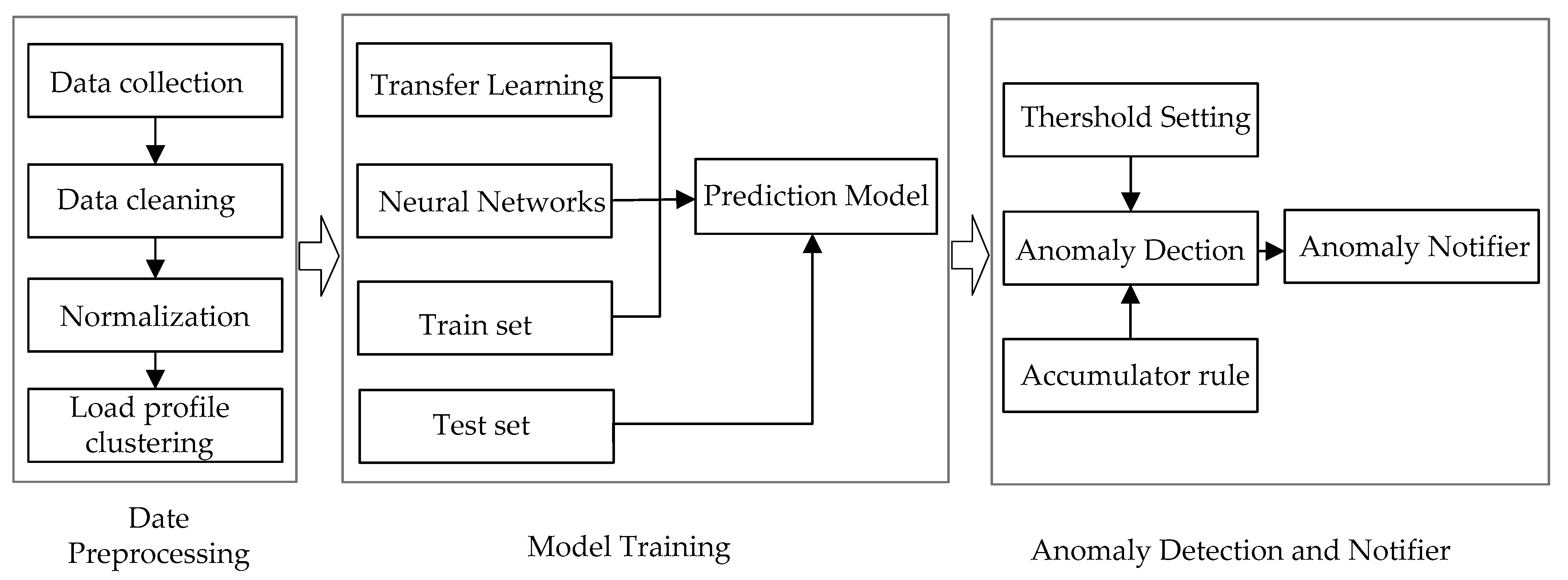
2. Data Preprocessing and Analysis

2.1. Data Cleaning

The operation data that the smart meter collected are not all valuable: some contain data that are incomplete, and thus worthless [26]. To mitigate the negative impact of noisy and incomplete data on the performance of the evaluation framework, this paper exploits the Local Outlier Factor [27] to remove erroneous values and interpolation method to recover the incomplete or worthless values:

$$\mathrm{f}({\mathrm{x}}_{\mathrm{i}})=\{\begin{array}{cc}\frac{{\mathrm{x}}_{\mathrm{i}-1}+{\mathrm{x}}_{\mathrm{i}+1}}{2}& {\mathrm{x}}_{\mathrm{i}}\in \mathrm{NaN},{\mathrm{x}}_{\mathrm{i}-1},{\mathrm{x}}_{\mathrm{i}+1}\notin \mathrm{NaN}\\ 0& {\mathrm{x}}_{\mathrm{i}}\in \mathrm{NaN},{\mathrm{x}}_{\mathrm{i}-1}\mathrm{or}{\mathrm{x}}_{\mathrm{i}+1}\notin \mathrm{NaN}\\ {\mathrm{x}}_{\mathrm{i}}& {\mathrm{x}}_{\mathrm{i}}\notin \mathrm{NaN}\end{array}$$

(1)

where x_i stands for the readings of the smart meter.

2.2. Normalization

The fluctuation range of meter readings is different for various customers, which is closely related to the electricity demand of users. For example, the power consumption of more populated households is generally one level higher than that of less populated households, but their power consumption patterns may have similarities. The use of metering values will reduce the effectiveness of clustering and TL, so do not input the power consumption directly into the prediction model. The activation function of the prediction model is more sensitive to the number near zero and the data has been normalized get the best cluster effect. In particular, the data were normalized by the MAX-MIN scaling method:

$$\mathrm{f}({\mathrm{x}}_{\mathrm{i}})=\frac{{\mathrm{x}}_{\mathrm{i}}-\min (\mathrm{x})}{\max (\mathrm{x})-\min (\mathrm{x})}$$

(2)

where x_i stands for the reading value, min(x) is the minimum value in x, and max(x) is the maximum value in x. After processing data through the standardized method, all data will fall within the range of [0, 1].

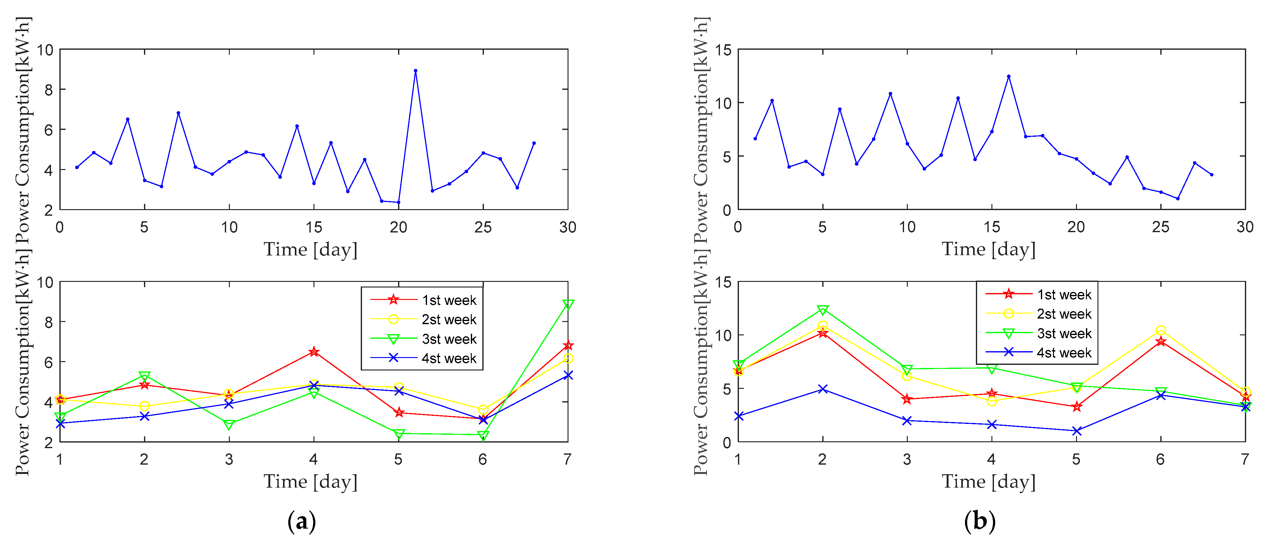
2.3. Electricity Curve Analysis

This paper analyzes the power consumption data collected by the smart meter. This dataset contains the power consumption of 128 customers within 420 days, which is provided by state grid Shanxi. Figure 2a shows the power consumption of the smart meter operate in normal state, which is arranged by day and week, respectively. With the curves arranged by day, the fluctuation of the power consumption can be observed but no regularity involved. The key features of power consumption data are hardly to capture by 1-D data which affect the efficient of neural networks. The regularity of the power consumption readings can be observed by arranging the data in week, in which the readings tend to peak on day 4 and day 7 every week and reach the trough on day 6. For the smart meter under normal operation, the regularity of its readings can be observed. The regularity for most meter readings was observed if aligning the readings of all the 12 months together [28].

In contrast, Figure 2b shows a reading of a malfunctioning smart meter in a month. Similar to Figure 2a, this paper plots the power consumption by date and week. It can be seen that the power consumption of the first two weeks fluctuates periodically and the reading tends to peak on day 2 and day 6. Since day 6 of the third week, the power consumption has been significantly reduced, and the power consumption has been kept at a low level. In this case, it can be judged that the user’s power consumption habits have changed or the operation state of the electric energy meter was malfunctioning.

However, with the support of abundant historical electricity data of users, accidental changes will not affect the overall trend. As long as the historical electricity data is sufficient, the user’s power consumption can be predicted. The prediction residual will be within a certain range if the electric energy meter operates normally. On the contrary, the characteristics of time series hidden in the electricity data changed accordingly with the change of operation mode of smart meter. As the meter operation changed, the prediction residual of the electricity data will be uncontrollable, so that the malfunctioning meter can be located.

3. Cluster-Based Chain Transfer Learning

TL is a machine learning method which aims at transferring knowledge the neural networks had already learnt. It can be applied to feature representation transfer, pre-trained neural networks transfer, and parameter transfer. This evaluation adopts parameter transfer, it aims to reduce the iterations of the prediction model for different learning domains which have similarity. The training time of the evaluation model is the product of the training time of a single prediction model and the number of meters. TL that merged into the model training process realizes the purpose that greatly reduce model overall training time and improve the operating efficiency of the framework. Cluster-based chain transfer learning (CBCTL) approach builds prediction models for abundant meters by applying clustering and TL. The efficiency of TL is improved by restricting the model parameters to be transferred in the same cluster. First, the prediction model focused on the internal feature rather than the size. It does not directly use power consumption values, but further transforms the readings through normalization. Each transformed data is treated as feature in the K-means clustering. Samples for all meters must start at same time. For each formed cluster, the model training process is applied with the meters within that cluster. Framework uses the meter data to determine the transfer path and the train set to train the neural network models. The TL path is indicated by the similarity of meters electrical data in each cluster. Select next meter which is most similar with the source meters. Setting the source meter as next model’s starting point obviously reduces the number of training epoch for optimizing hyperparameters.

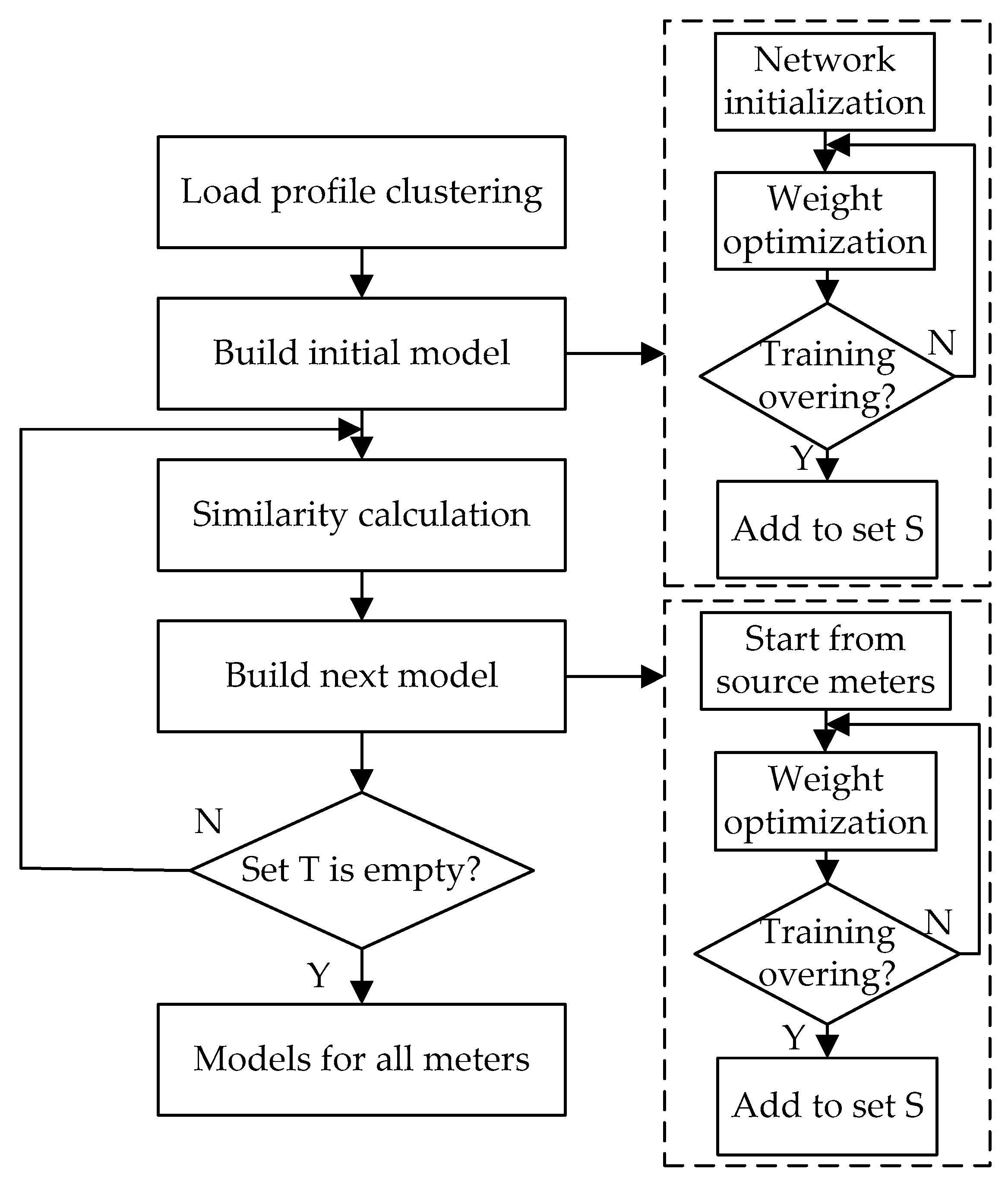
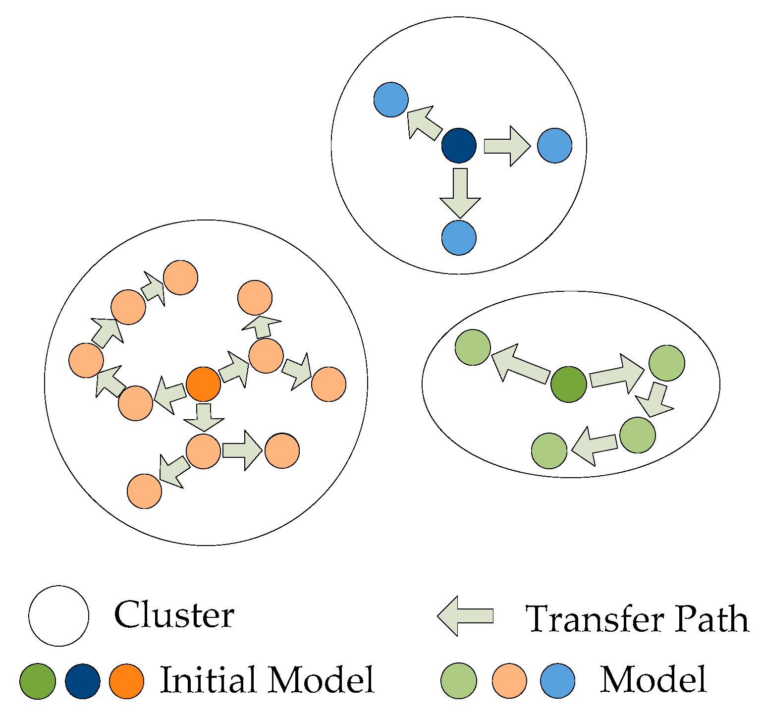
3.1. Load Profile Clustering

Faced with significant amounts of meters, it is an onerous task to establish the evaluation model. The weights learned during the initial model training were transferred from the source domain to the target domain. It is to expect that success will be higher if the two domains are more similar. Moreover, the accuracy of forecasting is higher if the transfer occurs between more similar meters. In addition to accuracy, higher similarity of the meters requires fewer training epochs which reduces the training time. K-means algorithm [29] is a classic distributed clustering algorithm. It randomly divides load profile into K clusters according to the profile and the Euclidean distance, which makes the daily power consumption of users in the cluster more similar with each cluster center. K-means clustering uses Euclidean distance as a distance measurement. The Euclidean distance between sample i and sample j is calculated as follows:

$${\mathrm{d}}_{\mathrm{Euel}}(\mathrm{x},\mathrm{y})=\sqrt{{\displaystyle \sum _{\mathrm{i}=1}^{\mathrm{n}}{{\displaystyle ({\mathrm{x}}_{\mathrm{i}}-{\mathrm{y}}_{\mathrm{i}})}}^2}}$$

(3)

The load profile is divided into K clusters, and the optimal number of clusters is determined by the elbow criterion [30]. The number of class is set from 1 to n, and n sum of squared errors (SSE) are calculated. According to the potential pattern of data, the SSE presents a rapid decline trend when the set number of clusters approaches the real number of class clusters. When the set number of class clusters exceeds the real number of class clusters, the SSE will continue to decline, and the decline will quickly slow down. By finding the inflection point during the descent, the K value can be better determined. The characteristics of the load profiles within the cluster are similar and the efficiency of TL is improved.

3.2. Transfer Learning

The determination of the TL direction of the model weights begins with the calculation of similarity between each pair of load curves within the cluster. The framework is interested in the characteristic of power consumption and not in the actual readings of smart meters [31]. The readings need to be scaled into the same range. The min-max normalization was performed in load profile clustering and similarity calculation continues using it scaled data.

R meters were clustered to a cluster, and the calculation of the similarity is a R*R upper oblique matrix. This similarity calculation matrix is expressed as S^R*R. The values in the matrix represent similarity between two meters, and the lower the value in the matrix the similar are the two customer’s power consumption characteristics. Three similarity calculation metrics are considered, including Euclidean, Cosign, and Manhattan distances.

$$\begin{array}{l}{\mathrm{d}}_{\mathrm{Euel}}(\mathrm{x},\mathrm{y})=\sqrt{{\displaystyle \sum _{\mathrm{i}=1}^{\mathrm{n}}{{\displaystyle ({\mathrm{x}}_{\mathrm{i}}-{\mathrm{y}}_{\mathrm{i}})}}^2}}\\ {\mathrm{d}}_{\mathrm{Cosign}}(\mathrm{x},\mathrm{y})=1-\frac{{\displaystyle {\sum }_{\mathrm{i}=1}^{\mathrm{n}}({\mathrm{x}}_{\mathrm{i}}\times {\mathrm{y}}_{\mathrm{i}})}}{\sqrt{{\displaystyle {\sum }_{\mathrm{i}=1}^{\mathrm{n}}{{\displaystyle ({\mathrm{x}}_{\mathrm{i}})}}^2}}\times \sqrt{{\displaystyle {\sum }_{\mathrm{i}=1}^n{{\displaystyle ({\mathrm{x}}_{\mathrm{i}})}}^2}}}\\ {\mathrm{d}}_{\mathrm{Manh}}(\mathrm{x},\mathrm{y})={\displaystyle \sum _{\mathrm{i}=1}^{\mathrm{n}}\left|{\mathrm{x}}_{\mathrm{i}}-{\mathrm{y}}_{\mathrm{i}}\right|}\end{array}$$

(4)

Denote set T and set S, where set T represents set of no prediction model and set S represents set of existing prediction models. To start with, none of the meters have a prediction model, all meters belong to the target set T and the source set S is empty. Denote prediction model as m₁, m₂, …, m_p, m_q, …, m_k $\in$ M, where M is the set of all prediction models and k is the number of models. Meter k data are denoted as d_k. Suppose that if these load curves have some similarities, so do the hyperparameters of the prediction model they have trained. Therefore, the training time of the modeling process can be reduced by setting the hyperparameters of similar meter prediction models as the training starting point. Figure 3 shows the framework of building the evaluation model. The TL process is as follows:

• Within each cluster, it is divided into source set S and target set T. TL starts with similarity calculation which gives similarities between each pair of meters within the cluster. Assume that meter p is the core of cluster and it was selected to build the initial prediction model m_p. The meter that has the maximum similarity to the initial meter p is selected as the TL target.
• The existing model m_p, which is trained by the power consumption data, is regarded as the starting point for training next prediction model m_q. Initial model m_p is trained by the target model dataset d_q to build the next model m_q. During the transferred process, the structure and hyperparameters of initial model remain the same. The weights for each model changed only in this situation that trained by its own dataset.
• The result of the training with the transferred model is the new source model m_q. The new built source model m_q, which is available for TL, was added to the source set S. For m_p, m_q, and m_k of the model that has already been built, the electrical data is attributed to the set S. For the electrical history data that does not have a model in the process, the data is attributed to set T.
• Next, the direction of the chain transfer is determined by calculating the similarity between set S and set T. Figure 4 shows the direction of chain transfer learning. The chain Transfer process ends with an empty set T, where all users have a well-trained evaluation model.

4. Evaluation Model

In this section, combining TL, Anomaly Detection Model (ADM), and RNN constructs a TL-ADM-RNN for time series anomaly detection.

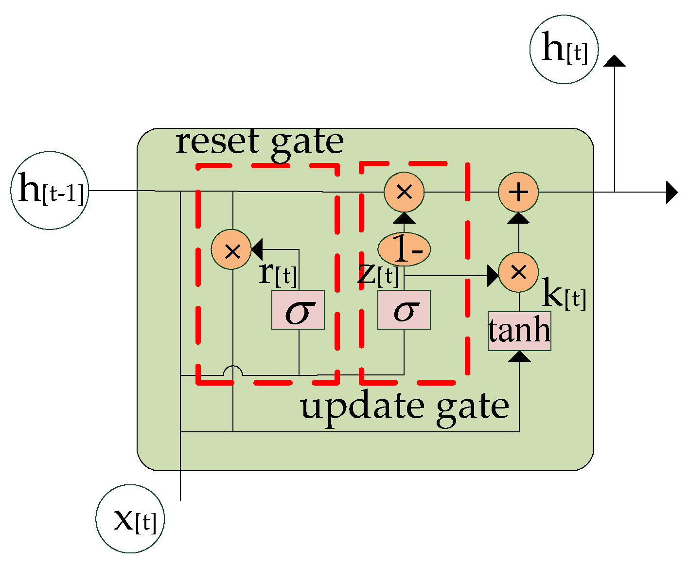
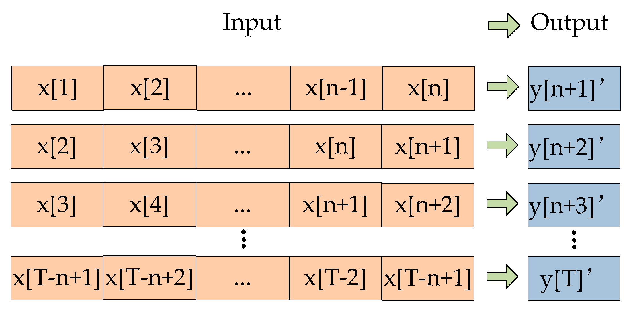
4.1. Prediction Model

RNN is selected as the core module of the prediction model. Gate recurrent unit (GRU) is a new generation of RNN, which is very similar to LSTM [32]. The structure diagram of GRU is provided in Figure 5. The integration method between new information and the previous memory was determined by Reset gate z, the amount of memory saved to the current time step was defined by update gate. The GRU differs from the LSTM cell in that it combines the cell storage and hidden states into a common hidden state h and also combines the input and forget gate into update gate z. GRU reduces the number of parameters and has long-term memory function. More importantly, it solves the problem of vanishing gradient. A reset gate r is introduced that mitigates the effect of the previous hidden state on the new hidden state, as shown in the update step in Formula (5). The formula in a single GRU unit is

$$\begin{array}{l}{\mathrm{r}}_{[\mathrm{t}]}=\mathrm{\sigma }({\mathrm{W}}_{\mathrm{xr}}{\mathrm{x}}_{[\mathrm{t}]}+{\mathrm{b}}_{\mathrm{xr}}+{\mathrm{W}}_{\mathrm{hr}}{\mathrm{h}}_{[\mathrm{t}-1]}+{\mathrm{b}}_{\mathrm{hr}})\\ {\mathrm{z}}_{[\mathrm{t}]}=\mathrm{\sigma }({\mathrm{W}}_{\mathrm{xz}}{\mathrm{x}}_{[\mathrm{t}]}+{\mathrm{b}}_{\mathrm{xz}}+{\mathrm{W}}_{\mathrm{hz}}{\mathrm{h}}_{[\mathrm{t}-1]}+{\mathrm{b}}_{\mathrm{hz}})\\ {\mathrm{k}}_{[\mathrm{t}]}=\tanh ({\mathrm{W}}_{\mathrm{xk}}{\mathrm{x}}_{[\mathrm{t}]}+{\mathrm{b}}_{\mathrm{xk}}+{\mathrm{r}}_{[\mathrm{t}]}\odot ({\mathrm{W}}_{\mathrm{hk}}{\mathrm{h}}_{[\mathrm{t}-1]}+{\mathrm{b}}_{\mathrm{hk}}))\\ {\mathrm{h}}_{[\mathrm{t}]}=(1-{\mathrm{z}}_{[\mathrm{t}]})\odot {\mathrm{k}}_{[\mathrm{t}]}+{\mathrm{z}}_{[\mathrm{t}]}\odot {\mathrm{h}}_{[\mathrm{t}-1]}\end{array}$$

(5)

where h_[t−1] is the hidden layer status at the previous moment, and h_[t] is the hidden layer information at the current moment. All of the weight matrices W* are updated using the error backpropagation algorithm according to the difference between the output value and the actual value, and b* denotes the bias vectors. $\odot$ indicates the element-wise multiplication between two vectors and indicates the element-wise multiplication between two vectors and $\mathrm{\sigma }$ expresses the activation function of the gate.

All models were built through the same neural networks approach, which were trained for a sufficient number of epochs ensuring that weights converge. To avoid getting stuck in a local minimum, a different set of the random initial values was chosen at the starting point of the training process. The input sequence x[1], …, x[T]is divided into smaller segments, which enable GRU to discover the internal periodicity in the consumption data. The segments pass through the GRU [33] to extract timing characteristics of the input vector obtain the prediction sequence y[1], …, y[N]. The schematic diagram of a sliding-window process is shown in Figure 6. As the train set has been passed through the model, the optimizer adjusts parameter. When the model reaches a fixed number of iterations or the MSE meets the requirements, the model is established.

The evaluation model adopts a grid-search method to address the HPO process. The hyperparameter range for the number of hidden layers and neurons is set, then the model is trained by traversing different combinations of hyperparameters and the model prediction error is calculated. By comparing the errors under different combination of hyperparameters, the hyperparameter with the best prediction effect is selected, and then the parameter settings of the model are determined.

4.2. Anomaly Detection Model

For a residential area after artificially detecting the meter state of the collected data, the smart meter operation state is normal as its default. The operation state of the meter can be determined by monitoring whether the data exceeds the threshold. In this paper, K-sigma and Confidence Interval are used to set the threshold of prediction residual. After training the prediction model, the K value or the C value is determined by the test set. The formula to calculate the prediction residual is shown below:

$$\mathrm{E}={\mathrm{W}}_{\mathrm{predict}}-{\mathrm{W}}_{\mathrm{rom}}$$

(6)

where E represents the daily residual error, ${\mathrm{W}}_{\mathrm{predict}}$ represents the daily electricity prediction, and ${\mathrm{W}}_{\mathrm{rom}}$ represents the daily reading of the meter.

Consumption data are divided into 80% train set and 20% test set. The prediction residual threshold is determined based on the residual of the test set. The ability of the model to predict the trend of power consumption is more important than the ability to predict accurately. The predictive capability of trained model is determined by the train set. Without the influence of changing the smart meter operation, the prediction residual will be within a certain range, which is determined by the prediction residual of the model itself. The model threshold is set by the performance of the test set in this segment.

4.2.1. K-Sigma

The upper and lower thresholds of the prediction residual are determined by K-Sigma, where the K value needs to be determined through the test set. The determination rule is to calculate the minimum K value that can satisfy the prediction residual of the test set. The threshold setting is intended to compare changes in the time series characteristics of the context and the prediction residual of normal data should belong to a normal range.

$$\begin{array}{l}\mathrm{Upper}\mathrm{threshold}={\mathrm{T}}_{\mathrm{mean}}+(\mathrm{K}\times {\mathrm{I}}_{\mathrm{range}})\\ \mathrm{Lower}\mathrm{threshold}={\mathrm{T}}_{\mathrm{mean}}-(\mathrm{K}\times {\mathrm{I}}_{\mathrm{range}})\end{array}$$

(7)

where T_mean represents the trimmed mean of the data, and the I_range represents the interquartile range of the data.

4.2.2. Confidence Interval

This paper sets the confidence interval of the prediction residual and obtains the confidence level by comparing the residual error in test set. The data for the known test set is collected in a normal state, and the confidence interval coefficients obtained from normal data are credible.

$$\begin{array}{l}\mathrm{Upper}\mathrm{threshold}=\overline{\mathrm{x}}-\mathrm{c}\frac{\mathrm{\sigma }}{\sqrt{\mathrm{n}}}\\ \mathrm{Lower}\mathrm{threshold}=\overline{\mathrm{x}}+\mathrm{c}\frac{\mathrm{\sigma }}{\sqrt{\mathrm{n}}}\end{array}$$

(8)

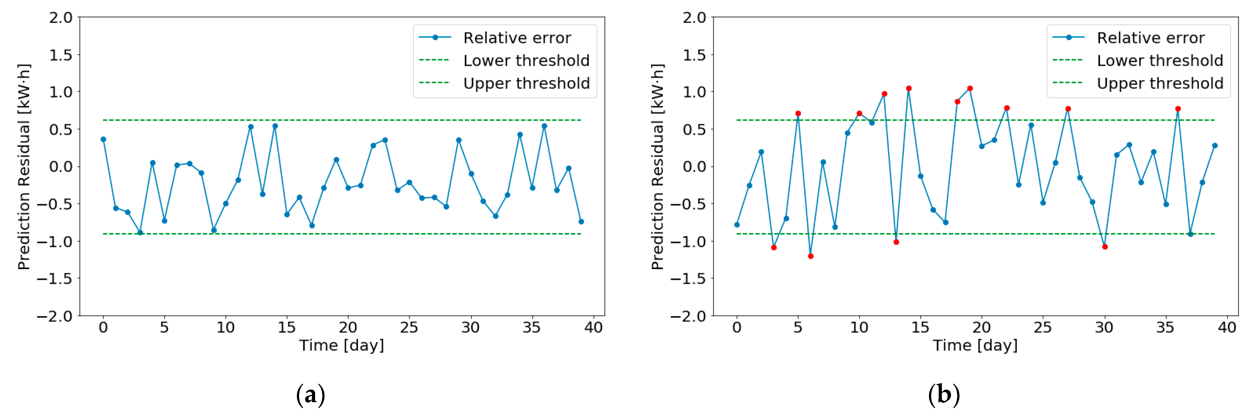
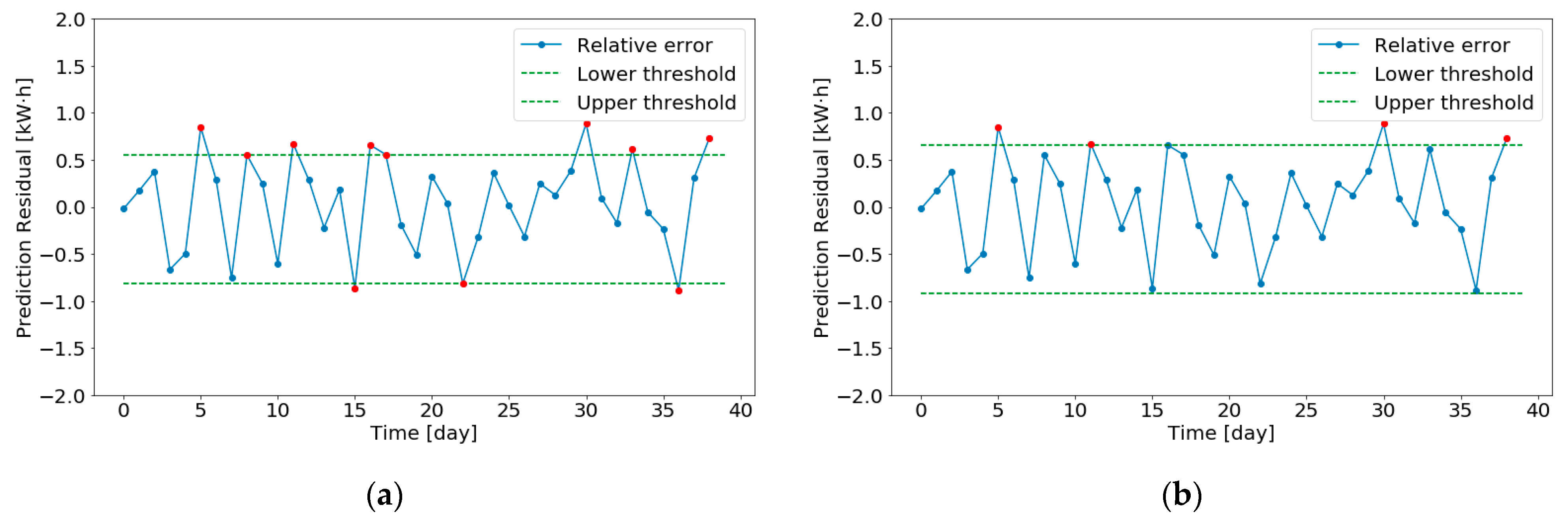
4.2.3. Abnormal Judgment

Abnormal judgment is a necessary part of anomaly detection. In [16], the submeters are defined as inaccurate if the predicted residual errors exceed threshold. In [17], it adopts three-sigma rule as the rule of abnormal judgment. The data are cited as abnormal when it exceeds outlier threshold. In [34], the state of the observed volume depended on whether the number of anomalies reported is sufficient. In this paper, the requirements of abnormal judgment are as follows:

• Abnormal detection requires reliability and effective identification when the operation state of meters changes.
• Abnormal detection needs to be robust, an abnormality caused by short-term power mutation or non-human causes during the operation of power system cannot be judged as abnormal.

The model defines outliers as prediction residual exceeding the upper and lower thresholds. Due to the volatility of power system, it is easy to produce false positives based on a single anomaly. This paper proposed the accumulator rule, whose rule was to require multiple outliers to occur in a short period of time before signaling anomaly. The use of accumulator improves decision performance. When the prediction residual exceeds the threshold range, the value of the accumulator grows. Conversely, the accumulator shrinks as the predicted residual within the threshold range [35]. The smart meter was judged to be abnormal when the prediction residual sends out a continuous abnormal signal for a certain period of time. The meter was determined as malfunctioning with the accumulator reaches the alarm value. In addition to the statistics of local anomalies, the monitoring rules are set for the whole data. When the relative error outliers exceed 20% of the total data, it is judged that the meter is malfunctioning.

5. Evaluation

The data were collected in the residential area of Shanxi, China and thoroughly inspected by humans; all of the meters are in good state. Empty rows and erroneous values were removed by data processing. It is assumed that all of the smart meters are in good operation state. To simulate a real-world residential area with malfunctioning meters, the malfunction was embedded manually. The offset for an inaccurate meter is a shift in the reading value, according to the technical specifications of smart meters. The relative error of the smart meter is more than 2%, which is judged to be abnormal. After the evaluation model was built and the human modified failure was injected. Selecting the consumption data to establish the evaluation model of operation state, the pre- and post-prediction residual as shown in Figure 7.

5.1. EX1

GRU and LSTM play an important role in RNN. Experiments show that sliding windows with different width have an important influence on the grasping and prediction of time series characteristics. The prediction accuracy of GRU and LSTM for power consumption was tested respectively in the case of 3, 7, 14, and 20 days, each experiment has run 30 times. The prediction accuracy was evaluated by mean square error (MSE), root mean square error (RMSE), mean absolute error (MAE), mean absolute percentage error (MAPE), and symmetric mean absolute percentage error (SMAPE). The results were summarized in

Table 1. Prediction accuracy of GRU under different windows.

GRU		MSE	RMSE	MAE	MAPE	SMAPE
3 Day	Mean	0.29	0.54	0.42	6.06	6.08
	Min	0.2	0.43	0.36	5.09	5.11
	Max	0.45	0.66	0.52	7.12	7.1
	Std	0.12	0.09	0.08	1.04	1.02
7 Day	Mean	0.28	0.52	0.39	5.81	5.72
	Min	0.18	0.43	0.32	4.79	4.61
	Max	0.44	0.66	0.51	6.64	7.07
	Std	0.08	0.07	0.06	0.79	0.78
14 Day	Mean	0.22	0.47	0.32	4.55	4.51
	Min	0.18	0.43	0.28	4.09	4.04
	Max	0.28	0.53	0.37	5.44	5.33
	Std	0.06	0.06	0.05	0.77	0.71
20 Day	Mean	0.56	0.73	0.5	7.58	7.15
	Min	0.24	0.49	0.31	4.64	4.51
	Max	0.86	0.92	0.64	9.39	8.8
	Std	0.25	0.18	0.13	2.06	1.87

and

Table 2. Prediction accuracy of LSTM under different windows.

LSTM		MSE	RMSE	MAE	MAPE	SMAPE
3 Day	Mean	0.62	0.72	0.62	7.26	7.12
	Min	0.43	0.56	0.42	6.16	6.06
	Max	0.81	0.94	0.84	8.2	8.18
	Std	0.19	0.2	0.24	1.12	1.08
7 Day	Mean	0.52	0.66	0.54	6.82	5.67
	Min	0.38	0.48	0.32	5.46	5.44
	Max	0.66	0.92	0.62	7.6	7.44
	Std	0.16	0.28	0.22	1.22	1.02
14 Day	Mean	0.42	0.58	0.37	5.26	5.43
	Min	0.32	0.45	0.26	4.36	4.28
	Max	0.54	0.68	0.44	6.22	6.08
	Std	0.13	0.12	0.09	0.98	0.96
20 Day	Mean	0.59	0.74	0.52	7.02	6.9
	Min	0.36	0.54	0.36	5.22	5.04
	Max	0.74	0.98	0.64	8.44	8.38
	Std	0.24	0.21	0.15	2.04	2.02

. The conclusions are as follows:

(1)

The prediction accuracy of GRU is higher overall than that of LSTM, and the model training time of GRU is shorter.

(2)

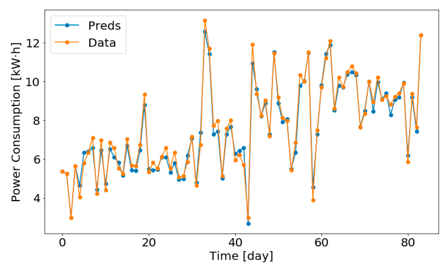
Through the comparison of MSE, RMSE, MAE, and other indicators in the process of predicting the power consumption, the prediction effect of GRU and 14-day sliding window is the best, and the prediction effect is shown in Figure 8.

(3)

The size of the sliding window affects the training time of the model, and the training time of the model increases with the expansion of the window.

5.2. EX2

The abnormal judgment of the evaluation model is based on the prediction residual. Residual threshold setting uses two methods: K-Sigma and Confidence interval. Both K and C values need to be set by the residual of the test set. For models built by different user data, thresholds for different models are different. This improves the generalization capability of the model. The error of fault injection is 3%, 5%, 7% and 10%. The model was experimented with two threshold settings. The results of the experiments can be found in Figure 9 and

Table 3. Prediction accuracy of GRU under different windows.

Failure Injection	K-Sigma	Confidence Interval
3%	abnormal	normal
5%	abnormal	abnormal
7%	abnormal	abnormal
10%	abnormal	abnormal

:

The results of the operation of the energy meter under different errors can be detected by model, and the K-Sigma method is more reliable.

5.3. EX3

The dataset is collected in a low-voltage network; 40 m are deployed in this system. This paper selects four meters and injects the fault offset artificially into the data. Data offsets as shown in

Table 4. Fault injection situation.

Meter Number	Failure Injection
9	3%
13	5%
22	7%
37	10%

:

The electric energy is regarded as a kind of generalized flow which satisfies the conservation law, so the electric energy meter, water meter, gas meter, and other conventional flow meters are abstracted as a kind of generalized flow meters. Under the flow conservation agreement, the actual flow increment of the master meter is equal to the sum of the increments of each sub meter in the same period, thus constituting (8):

$$\mathrm{Y}(\mathrm{i})(1-{\mathrm{e}}_{\mathrm{z}})={\displaystyle {\sum }_{\mathrm{j}=1}^{\mathrm{P}}{\mathrm{Q}}_{\mathrm{j}}(\mathrm{i})(1-{\mathrm{e}}_{\mathrm{j}})+}{\mathrm{e}}_{\mathrm{y}}\mathrm{Y}(\mathrm{i})(1-{\mathrm{e}}_{\mathrm{z}})+\mathrm{e}0$$

(9)

where $\mathrm{Y}(\mathrm{i})$ is the reading of the master meter, ${\mathrm{Q}}_{\mathrm{j}}(\mathrm{i})$ is the reading of the sub-meter, ${\mathrm{e}}_{\mathrm{z}}$ is the operation error of the master meter, measured on-site or laboratory, ${\mathrm{e}}_{\mathrm{j}}$ is the operation error of the sub-meter, ${\mathrm{e}}_{\mathrm{y}}$ is the line loss rate of the area, and $\mathrm{e}0$ is the fixed loss of the area.

$${\mathrm{e}}_{\mathrm{j}}=\frac{{\mathrm{Q}}_{\mathrm{j}}-{\mathrm{x}}_{\mathrm{j}}}{{\mathrm{Q}}_{\mathrm{j}}}$$

(10)

where ${\mathrm{x}}_{\mathrm{j}}$ represents the actual consumption of the meter.

Figure 10 shows the results of error estimator. It can be seen that the error of meter 28 is calculated at 3.19%, the error of meter 37 is calculated at −4.9%, and the other two abnormal meters cannot be found. In this paper, the above four abnormal smart meters were detected by the model this paper proposed. The results were shown in

Table 5. Results of evaluation model.

Meter Number	Failure Injection
9	abnormal
13	abnormal
22	abnormal
37	abnormal

. For meter 9, the model prediction residual was shown in Figure 11. The conclusion of the comparison as following:

(1)

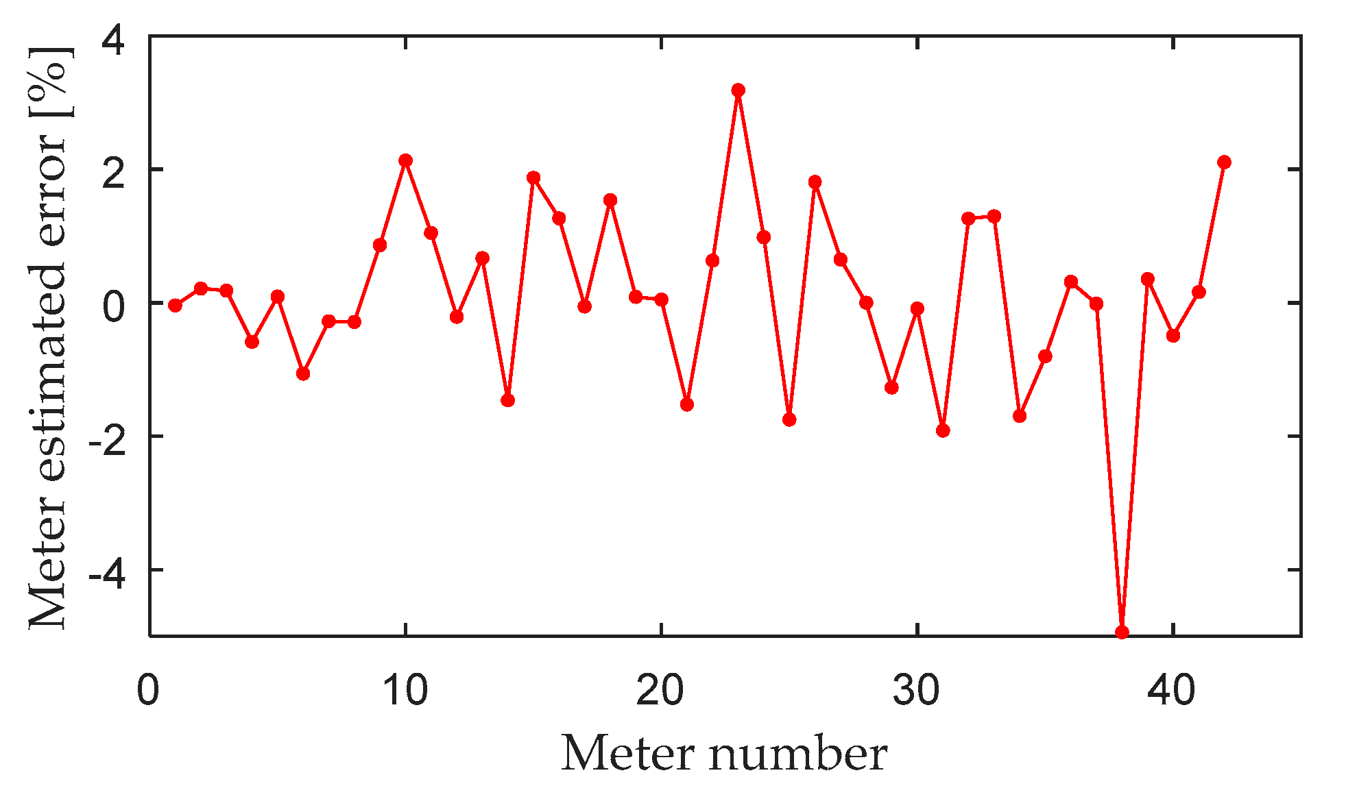
When the cluster-based error estimation matrix of smart meter is constructed, the measurement result is the average operation error of the whole measurement cycle. The historical data will affect the recent state of smart meters. The error estimation of smart meter has no timeliness.

(2)

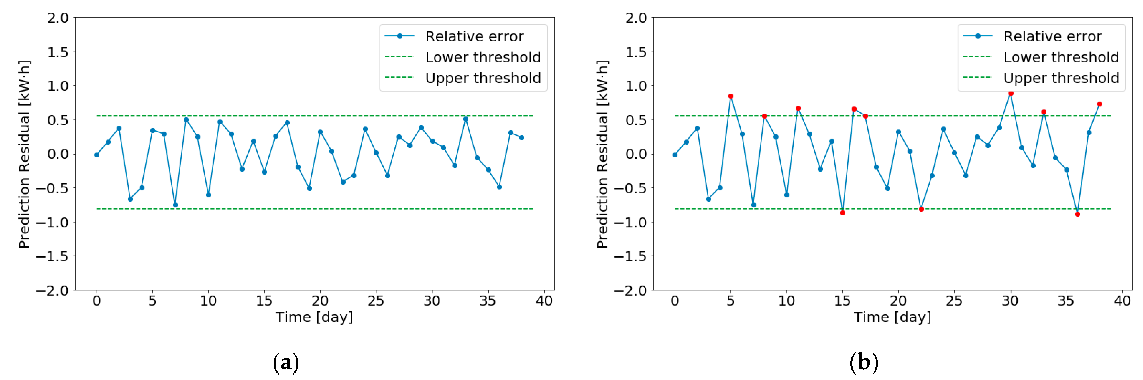
The evaluation model of smart meters evaluates meters in real-time. The abnormal state of smart meter can be identified quickly, sensitively, and reliably when the characteristics of power consumption data change combined with abnormal judgment.

6. Conclusions and Future Work

In this paper, the key technology of smart meter state evaluation is studied and an online evaluation method of smart meter operation state is proposed. The state evaluation model of the smart meters is established based on the historical consumption data. The power consumption of users was accurately predicted by the RNN. When the operation state of the smart meter changed, the model can accurately find the malfunctioning smart meter. TL greatly reduces the time to establish the model and improves the efficiency of model training. The flexibility of threshold setting makes it more suitable for the condition monitoring of smart meter. According to the actual data of a certain station in Shanxi Province, the evaluation model of the smart meter is established and evaluation of operation state for smart meter is carried out. The evaluation can provide effective technical support for daily operation, maintenance management, state evaluation of smart meters and accurate replacement strategy which greatly improve the intelligent management level and work efficiency of power operation management department.

References

1. Yu, X.; Xue, Y. Smart Grids: A Cyber–Physical Systems Perspective. Proc. IEEE 2016, 104, 1–13. [Google Scholar] [CrossRef]
2. Saputro, N.; Akkaya, K. Investigation of Smart Meter Data Reporting Strategies for Optimized Performance in Smart Grid AMI Networks. IEEE Internet Things 2017, 4, 894–904. [Google Scholar] [CrossRef]
3. Ekanayake, J.B.; Jenkins, N.; Liyanage, K.; Wu, J.; Yokoyama, A. Smart Grid: Technology and Applications; Wiley & Sons: Hoboken, NJ, USA, 2012. [Google Scholar]
4. Alahakoon, D.; Yu, X. Smart Electricity Meter Data Intelligence for Future Energy Systems: A Survey. IEEE Trans. Ind. Inform. 2016, 12, 425–436. [Google Scholar] [CrossRef]
5. Xiaojuan, P.; Lei, W.; Zhengsen, J.; Xuewei, W.; Hongtao, H.; Lijuan, L. Evaluation of digital energy meter error by Monte Carlo method. In Proceedings of the 2016 Conference on Precision Electromagnetic Measurements (CPEM 2016), Ottawa, ON, Canada, 10–15 July 2016; pp. 1–2. [Google Scholar]
6. Zhang, Z.; Gong, H.; Li, C.; Wang, Z.; Xiang, X. Research on estimating method for the smart electric energy meter’s error based on parameter degradation model. IOP Conf. Ser. Mater. Sci. Eng. 2018, 366, 012065. [Google Scholar] [CrossRef]
7. Fangxing, L.; Qing, H.; Shiyan, H.; Lei, W.; Zhengsen, J. Estimation of Smart Meters Errors Using Meter Reading Data. In Proceedings of the 2018 Conference on Precision Electromagnetic Measurements (CPEM 2018), Paris, France, 8–13 July 2018; pp. 1–2. [Google Scholar]
8. Liu, F.; Liang, C.; He, Q. A Data-Based Approach for Smart Meter Online Calibration. Acta IMEKO 2020, 9, 32. [Google Scholar] [CrossRef]
9. Kong, X.; Ma, Y.; Zhao, X.; Li, Y.; Teng, Y. A Recursive Least Squares Method with Double-Parameter for Online Estimation of Electric Meter Errors. Energies 2019, 12, 805. [Google Scholar] [CrossRef] [Green Version]
10. Kim, J.Y.; Hwang, Y.M.; Sun, Y.G.; Sim, I.; Kim, D.I.; Wang, X. Detection for Non-Technical Loss by Smart Energy Theft With Intermediate Monitor Meter in Smart Grid. IEEE Access 2019, 7, 129043–129053. [Google Scholar] [CrossRef]
11. Ying, C.Y.; Jie, D.; Feng, Z.; Ji, X.; Xiao, Y.H. Application of variable weight fuzzy analytic hierarchy process in evaluation of electric energy meter. In Proceedings of the 2017 IEEE 2nd Advanced Information Technology, Electronic and Automation Control Conference (IAEAC), Chongqing, China, 25–26 March 2017; pp. 1985–1989. [Google Scholar]
12. Berhane Araya, D. Collective Contextual Anomaly Detection for Building Energy Consumption. In Proceedings of the 2016 International Joint Conference on Neural Networks (IJCNN), Vancouver, BC, Canada, 24–29 July 2016; pp. 511–518. [Google Scholar]
13. Yaffee, R.A.; McGee, M. An Introduction to Time Series Analysis and Forecasting: With Applications of SAS® and SPSS®; Elsevier: Amsterdam, The Netherlands, 2000. [Google Scholar]
14. Tian, Y.; Sehovac, L.; Grolinger, K. Similarity-Based Chained Transfer Learning for Energy Forecasting With Big Data. IEEE Access 2019, 7, 139895–139908. [Google Scholar] [CrossRef]
15. Cui, W.; Wang, H. Anomaly detection and visualization of school electricity consumption data. In Proceedings of the 2017 IEEE 2nd International Conference on Big Data Analysis (ICBDA), Beijing, China, 10–12 March 2017; pp. 606–611. [Google Scholar]
16. Liu, M.; Liu, D.; Sun, G.; Zhao, Y.; Wang, D.; Liu, F.; Fang, X.; He, Q.; Xu, D. Deep Learning Detection of Inaccurate Smart Electricity Meters: A Case Study. IEEE Ind. Electron. Mag. 2020, 14, 79–90. [Google Scholar] [CrossRef]
17. Zheng, Z.; Yang, Y.; Niu, X.; Dai, H.-N.; Zhou, Y. Wide and deep convolutional neural networks for electricity-theft detection to secure smart grids. IEEE Trans. Ind. Inform. 2017, 14, 1606–1615. [Google Scholar] [CrossRef]
18. Amarbayasgalan, T.; Pham, V.H.; Theera-Umpon, N.; Ryu, K.H. Unsupervised anomaly detection approach for time-Series in multi-domains using deep reconstruction error. Symmetry 2020, 12, 1251. [Google Scholar] [CrossRef]
19. Sehovac, L.; Nesen, C.; Grolinger, K. Forecasting building energy consumption with deep learning: A sequence to sequence approach. In Proceedings of the 2019 IEEE International Congress on Internet of Things (ICIOT), Milan, Italy, 8–13 July 2019; pp. 108–116. [Google Scholar]
20. Kou, Z.; Fang, Y. An Improved Residual Network for Electricity Power Meter Error Estimation. Int. J. Pattern Recognit. Artif. Intell. 2019, 33, 1959024. [Google Scholar] [CrossRef]
21. Kim, T.-Y.; Cho, S.-B. Web traffic anomaly detection using C-LSTM neural networks. Expert Syst. Appl. 2018, 106, 66–76. [Google Scholar] [CrossRef]
22. Neshat, M.; Nezhad, M.M.; Abbasnejad, E.; Mirjalili, S.; Tjernberg, L.B.; Astiaso Garcia, D.; Alexander, B.; Wagner, M. A deep learning-based evolutionary model for short-term wind speed forecasting: A case study of the Lillgrund offshore wind farm. Energy Convers. Manag. 2021, 236, 114002. [Google Scholar] [CrossRef]
23. Wang, J.Q.; Du, Y.; Wang, J. LSTM based long-term energy consumption prediction with periodicity. Energy 2020, 197, 117197. [Google Scholar] [CrossRef]
24. Duan, J.; Zuo, H.; Bai, Y.; Duan, J.; Chang, M.; Chen, B. Short-term wind speed forecasting using recurrent neural networks with error correction. Energy 2021, 217, 119397. [Google Scholar] [CrossRef]
25. Qu, Z.; Xu, J.; Wang, Z.; Chi, R.; Liu, H. Prediction of electricity generation from a combined cycle power plant based on a stacking ensemble and its hyperparameter optimization with a grid-search method. Energy 2021, 227, 120309. [Google Scholar] [CrossRef]
26. García, S.; Ramírez-Gallego, S.; Luengo, J.; Benítez, J.M.; Herrera, F. Big data preprocessing: Methods and prospects. Big Data Anal. 2016, 1, 9. [Google Scholar] [CrossRef] [Green Version]
27. Ma, H.; Hu, Y.; Shi, H. Fault detection and identification based on the neighborhood standardized local outlier factor method. Ind. Eng. Chem. Res. 2013, 52, 2389–2402. [Google Scholar] [CrossRef]
28. Jokar, P.; Arianpoo, N.; Leung, V.C. Electricity theft detection in AMI using customers’ consumption patterns. IEEE Trans. Smart Grid 2015, 7, 216–226. [Google Scholar] [CrossRef]
29. Kodinariya, T.; Makwana, P. Review on Determining of Cluster in K-means Clustering. Int. J. Adv. Res. Comput. Sci. Manag. Stud. 2013, 1, 90–95. [Google Scholar]
30. Syakur, M.A.; Khotimah, B.K.; Rochman, E.M.S.; Satoto, B.D. Integration K-Means Clustering Method and Elbow Method For Identification of The Best Customer Profile Cluster. IOP Conf. Ser. Mater. Sci. Eng. 2018, 336, 012017. [Google Scholar] [CrossRef] [Green Version]
31. Sun, J.; Cao, X.; Liang, H.; Huang, W.; Chen, Z.; Li, Z. New Interpretations of Normalization Methods in Deep Learning. Proc. AAAI Conf. Artif. Intell. 2020, 34, 5875–5882. [Google Scholar]
32. Zheng, J.; Xu, C.; Zhang, Z.; Li, X. Electric load forecasting in smart grids using long-short-term-memory based recurrent neural network. In Proceedings of the 2017 51st Annual Conference on Information Sciences and Systems (CISS), Baltimore, MD, USA, 22–24 March 2017; pp. 1–6. [Google Scholar]
33. Malekizadeh, M.; Karami, H.; Karimi, M.; Moshari, A.; Sanjari, M. Short-term load forecast using ensemble neuro-fuzzy model. Energy 2020, 196, 117127. [Google Scholar] [CrossRef]
34. Zanetti, M.; Jamhour, E.; Pellenz, M.; Penna, M.; Zambenedetti, V.; Chueiri, I. A Tunable Fraud Detection System for Advanced Metering Infrastructure Using Short-Lived Patterns. IEEE Trans. Smart Grid 2019, 10, 830–840. [Google Scholar] [CrossRef]
35. Shipmon, D.T.; Gurevitch, J.M.; Piselli, P.M.; Edwards, S.T. Time series anomaly detection; detection of anomalous drops with limited features and sparse examples in noisy highly periodic data. arXiv 2017, arXiv:1708.03665. [Google Scholar]
Figure 1. Workflow of malfunctioning smart meter detection.
Energies 14 04674 g001
Figure 2. (a) Analysis of electricity curve of electricity meter in normal operation state. (b) Analysis of electricity curve of electricity meter in abnormal operation state.
Energies 14 04674 g002
Figure 3. Evaluation model framework.
Energies 14 04674 g003
Figure 4. Chain transfer learning direction.
Energies 14 04674 g004
Figure 5. GRU structure diagram.
Energies 14 04674 g005
Figure 6. Schematic diagram of a sliding-window process.
Energies 14 04674 g006
Figure 7. (a) State monitoring diagram of normal smart meter. (b) State monitoring diagram of smart meter after adding fault.
Energies 14 04674 g007
Figure 8. Prediction effect of GRU under 14-day sliding window.
Energies 14 04674 g008
Figure 9. (a) The model with K-sigma in 3% fault injection. (b) The model with Confidence interval in 3% fault injection.
Energies 14 04674 g009
Figure 10. Results of cluster-based operation error method of electric energy meters.
Energies 14 04674 g010
Figure 11. (a) The residual output results of the meter 9 in normal state. (b) The output result of the residual error of the meter 9 in the 3% error injection model.
Energies 14 04674 g011