Assessing Hydrokinetic Energy in the Mexican Caribbean: A Case Study in the Cozumel Channel

Abstract

This paper presents a techno-economic assessment of hydrokinetic energy of Cozumel Island, where ocean currents have been detected, but tourist activities are paramount. The main objective of this research is to identify devices that have been used to harvest hydrokinetic power elsewhere and perform an economic analysis as to their implementation in the Mexican Caribbean. First, the energy potential of the area was evaluated using simulated data available through the HYCOM consortium. Then, for four pre-commercial and commercial turbines, technical and economic analyses of their deployments were performed. Socio-environmental constraints were reviewed and discussed. Three optimal sites were identified, with an average annual hydrokinetic energy density of 3–6 MWh/m²-year. These sites meet the socio-environmental requirements for marine kinetic energy harvesting. Of the turbines considered in the analysis, the best energy price/cost ratio is that of SeaGen device, with a maximum theoretical energy extraction of 1319 MWh/year with a Capacity Factor of 12.5% and a Levelised Cost of Energy (LCOE) of 1148 USD/MWh. Using this device, but assuming a site-specific design that achieves at least 25% of Capacity Factor, 20-year useful life, and a discount rate of 0.125, the LCOE would be 685.6 USD/MWh. The approach presented here can be applied for techno-economic analyses of marine turbines in other regions.

1. Introduction

The wide range of renewable energies are increasingly seen as feasible alternatives to generate electricity. Some of these technologies are well documented and in an advanced stage, while others are still in their infancy [1,2]. Among the latter, ocean energy has recently gained attention due to the diverse harvesting possibilities it offers [3,4,5]. In a project involving any of these ocean energy sources, three steps are required: (1) a theoretical assessment of resources; (2) a technical assessment, considering the devices available; and (3) a practical assessment, including in-site evaluations [6,7].

In some parts of the world, ocean currents exist that can be harnessed to provide energy. There are eight main regions with an average kinetic energy flux of over 0.5 kW/m², (HYCOM [8] data, 2009–2012, at a depth of 20 m); the South African coast (Agulhas Current), the southeast U.S. and Mexican coasts (Gulf Stream-Cape Hatteras, Florida current-Florida Straits and Yucatan current in Cozumel), Japan (Kuroshio current), Indonesia, Somalia, Brazil (Brazil Coastal Current), Madagascar (Madagascar Currents), and Australia (South West Rocks). At four of these sites, the direction of the current is persistent and there are no reverse flows: north of Madagascar, off part of the Brazilian coast, and Florida current and Yucatan current [9].

Previous published works on energy harvesting from some of the most promising ocean current systems describe projects using the Agulhas current, off the south coast of Africa [10,11], the Kuroshio current near the coasts of Japan and Taiwan [12,13] and the Gulf Stream [14,15] off the north American east coast [16], and a small part of southern Mexico [17].

Marais et al. [18] and Meyer and Van Niekerk [19] performed resource assessments to verify the theoretical power that could be extracted from the Agulhas current. Wright et al. [20] carried out a feasibility study to identify possibilities for energy extraction, while [21] performed an economic assessment of this off the east coast of South Africa.

With respect to the Kuroshio current, an assessment of available power was performed for Green Island, Japan, [22,23] and Miyake Island off eastern Taiwan [24,25]. Other works discuss harvesting off the coast of Japan [26,27]. While for Taiwan, a complete energy assessment project was published by [28].

In 2014, the time series of the current velocity in the Gulf Stream-Cape Hatteras region, at a depth of 75 m, were recorded, giving an annual average power of 1000 W/m² (8.76 MWh/m²-year) [9]. In this paper, the authors then compared their data with numerical results obtained with HYCOM, finding that the average HYCOM speed was 3% greater than the field measurements. Off the South African coast, HYCOM predicts the maximum kinetic energy flux per unit area (density power) as 1830 W/m², with current direction reversals 1.5% of the time, while in-site measurements displayed a density power of 1760 W/m² [29].

Several theoretical assessments have been carried out for the Gulf Stream, off the coasts of USA, including a general assessment by [30,31] and others that focused on the coast of Florida [16,32,33,34] and off the coast of North Carolina [35]. A small part of the Gulf Stream system also affects the south of the Mexican Caribbean, particularly the state of Quintana Roo. Hernández-Fontes et al. [6] performed a theoretical identification of resources in southern Mexico, finding that ocean energy harvesting could be profitable at some sites off Cozumel island, in Quintana Roo, where there is both high availability and persistence of the ocean current. Alcérreca-Huerta et al. [17] evaluated potential sites off Cozumel, and [36] discussed the technical possibilities of using low-speed turbines there.

In the Mexican Caribbean there is a persistent current that can generate a power density of over 176 W/m² (1.54 MWh/m²-year) to 512 W/m² (4.48 MWh/m²-year), which is available more than 50% of the time [6]. In a specific study in the area off the west cost of Cozumel Island, Alcérreca-Huerta et al. [17] mentions 300–1000 W/m² (2.63–8.76 MWh/m²-year) and other sites with 1000–2500 W/m² (8.76–21.9 MWh/m²-year). These results were for the −10 to −30 m isobaths and suggest that a suitable site for the installation of a turbine may be in front of International Airport of Island of Cozumel, where it is estimated that nearly 3.2 MW could be generated.

Comparing energy densities with tide currents, the high annual energy densities off Jeonnam Province, on the western tip of southwest Korea, of 23 MWh/m²-year (2625.6 W/m²) at Uldolmok; 15 MWh/m²-year (1712.3 W/m²) at Maenggol Sudo; 9.2 MWh/m²-year (1050 W/m²) at Geocha Sudo; 8.8 MWh/m²-year (1004 W/m²) at Jaingjuk Sudo; and 16 MWh/m²-year (1826.5 W/m²), in Gyudong Suro, in Gyeonggi Province’s Gyeonggi Bay, were found [37].

Quintana Roo may be the most suitable part of Mexico for the successful implementation of hydrokinetic energy projects. Because of the tourism activities in this region [38], the economy in Cozumel seems more stable than that of other regions in Mexico where there are ocean energy resources, but the socioeconomic and environmental restrictions present strong barriers for ocean energy conversion [39]. Based on the results of [40], some of the most attractive sites for device deployment are close to the coast off Puerto Morelos and the east coast of Cozumel island.

Although previous works have focused on assessing theoretical potential and identifying potential sites for projects in Mexico (e.g., [6]), there have been no techno-economic studies that describe the feasibility of using mature technologies for ocean current energy conversion in the most prospective regions, such as in Cozumel. In this region, availability and persistence of hydrokinetic energy has been identified; however, this is a region with active tourist activities where social and environmental constrains should also be taken into account. Furthermore, more technical analysis, including feasibility studies of existing devices in pre and commercial stages are still needed.

To help fill this knowledge gap, a techno-economic assessment of energy from ocean currents off Cozumel, Mexico, is presented in this paper as a continuation of former theoretical resource assessments (e.g., [6]). The main objective of the work was to identify which device has the best cost–benefit relationship. In addition, technical factors related to the design of devices commonly used for tidal energy were evaluated, and environmental, touristic, and social considerations, relevant in the study zone, are also discussed.

It is hoped that the work presented here will be useful in bringing to fruition projects in marine current energy generation in Mexico. The manuscript is organized as follows: Section 2 presents the methodology, including the description of the four hydrokinetic devices, descriptions of the databases employed, as well as the analytical methods used in the techno-economic analysis. The results of the technical and economic analysis are presented in Section 3 and Section 4, respectively. Section 4 includes the estimated Capacity Factors of the devices considered as well as the Levelised Cost of Energy (LCOE). In Section 5, the main technical, social, and environmental challenges are described. Finally, the main conclusions and future perspectives are summarized in Section 6.

2. Methodology

To assess the objectives of the present work, a brief review of the state of the art of the technology used for hydrokinetic energy conversion of ocean currents was performed, including previous studies of energy potential in the study area. Considering the available energy power of ocean currents in this region and technical information from different devices, four devices were selected for the economic analysis, which estimates the most convenient project costs for the planning and installation of the devices in the study area. The feasibility of each turbine was discussed, including technical challenges related to installation, mooring, soil, climate, and distance to infrastructure. Finally, challenges related to environmental restrictions, sites of touristic interest, military activities, marine transportation routes, and possible social resilience in the region of interest, were described.

2.1. Case Study

2.1.1. The Present Energy Scenario in the Mexican Caribbean

The Mexican government has promised that by 2024, ~35% of the nation’s electricity demand will be met from renewable energy sources. Various energy sources are considered, including that from tides and ocean currents. The Mexican Secretary for Energy established the aim to reduce the use of fossil fuels to 65%, 60%, and 50% by the years 2024, 2035, and 2050, respectively.

In a report on electricity consumption by the Mexican System of Energy Information [41] in the state of Quintana Roo, where Cozumel is found, it was shown to have consumed 3224 GWh in 2007, and 4504 GWh In 2017; an average increase of 128 GWh.

For the same years (2007–2017), electricity was generated within Quintana Roo state using low-efficiency turbogas technology, 41.0 GWh and 110.37 GWh, respectively. In another study, the average annual growth in electricity consumption in the Yucatán peninsula (Campeche, Yucatán and Quintana Roo states) was estimated at ~3.9%, for 2018–2032 (Figure 1a,b), the region with the highest growth in electricity consumption in Mexico. In particular, it is predicted that Cozumel will increase its grid capacity from 48 MW to 194 MW by 2024 [42].

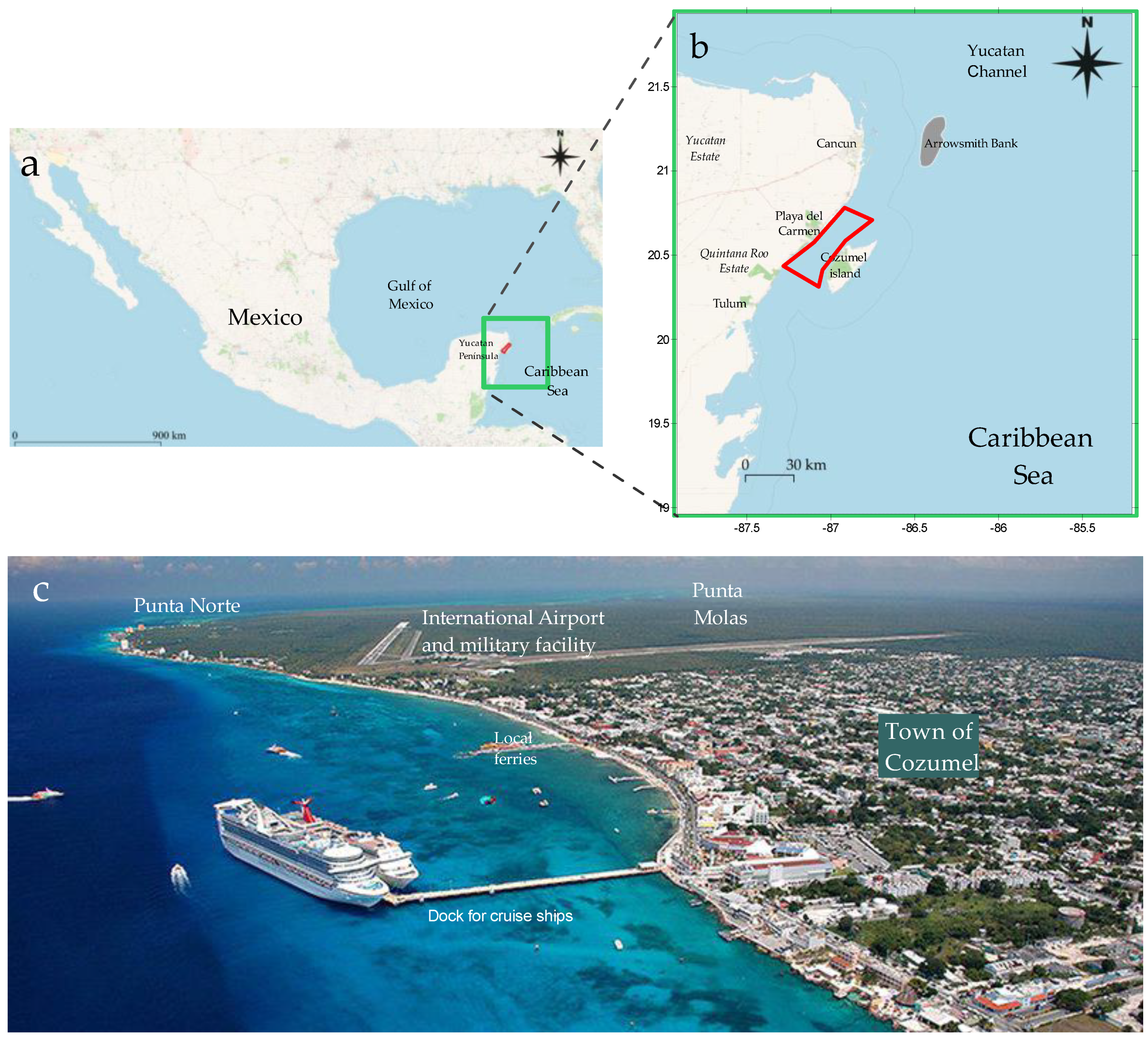
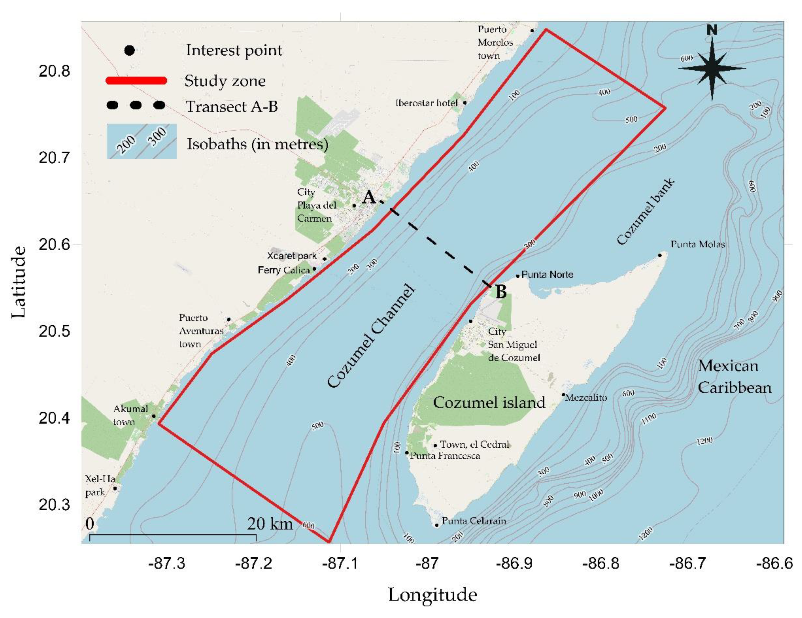
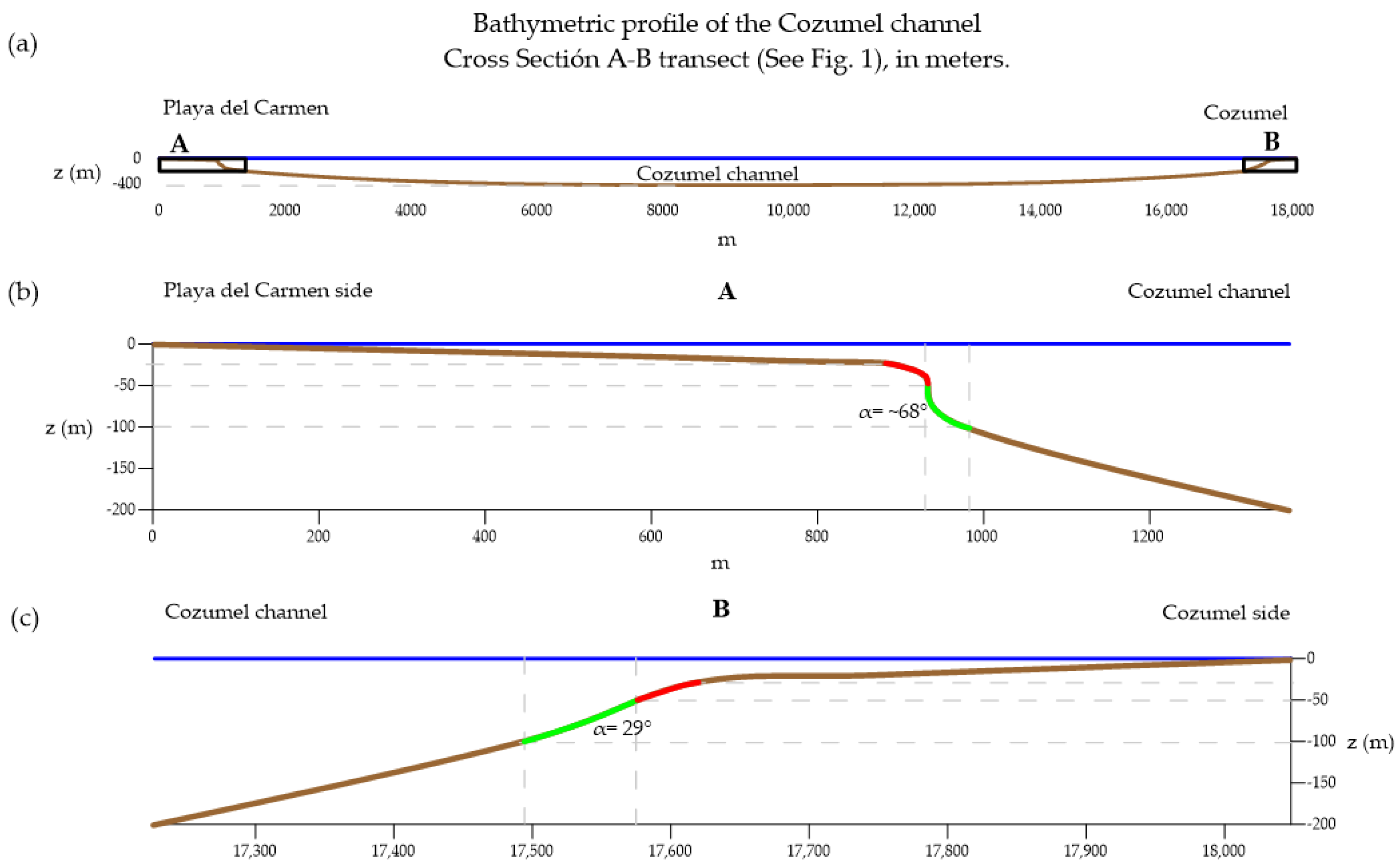
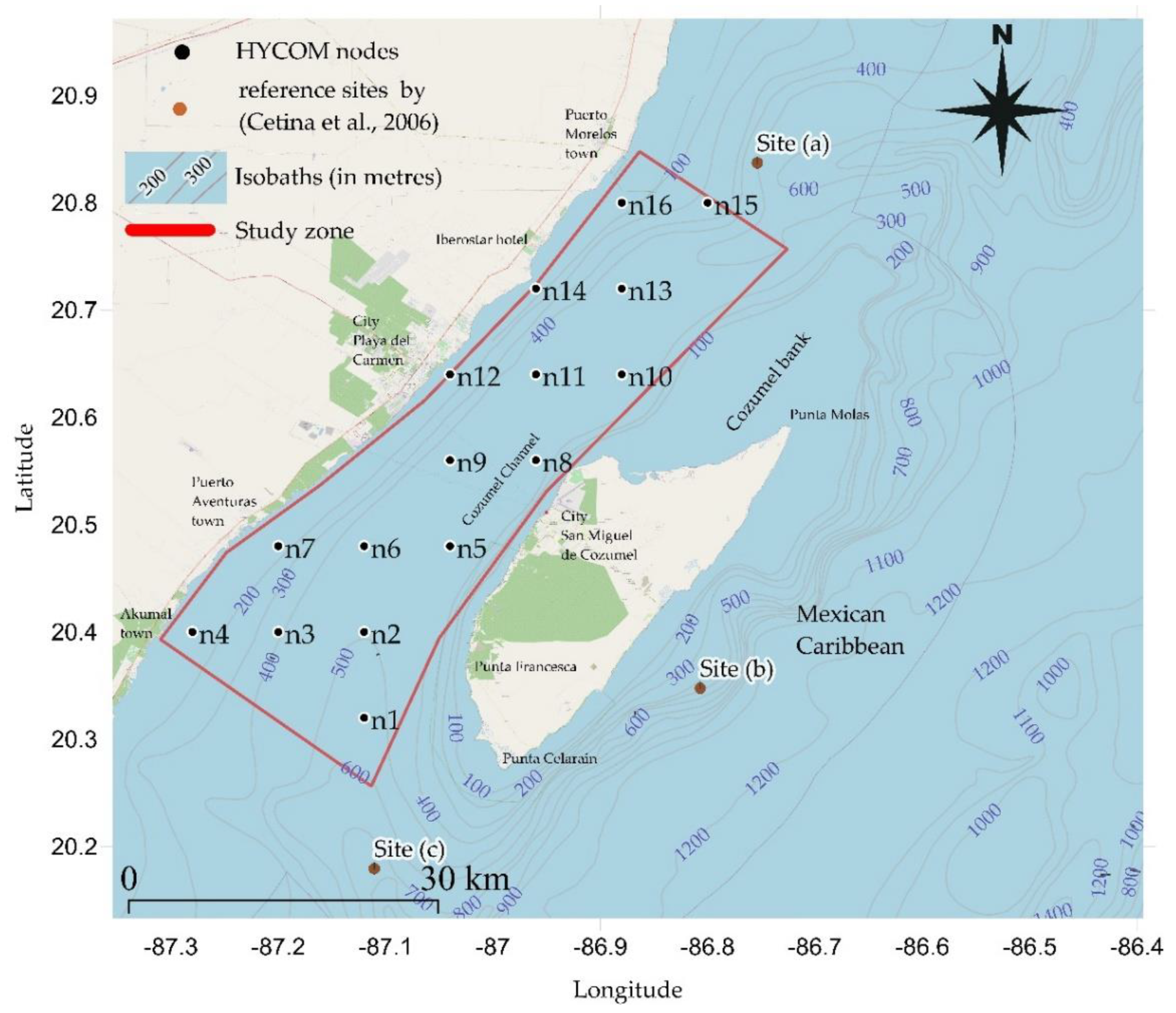
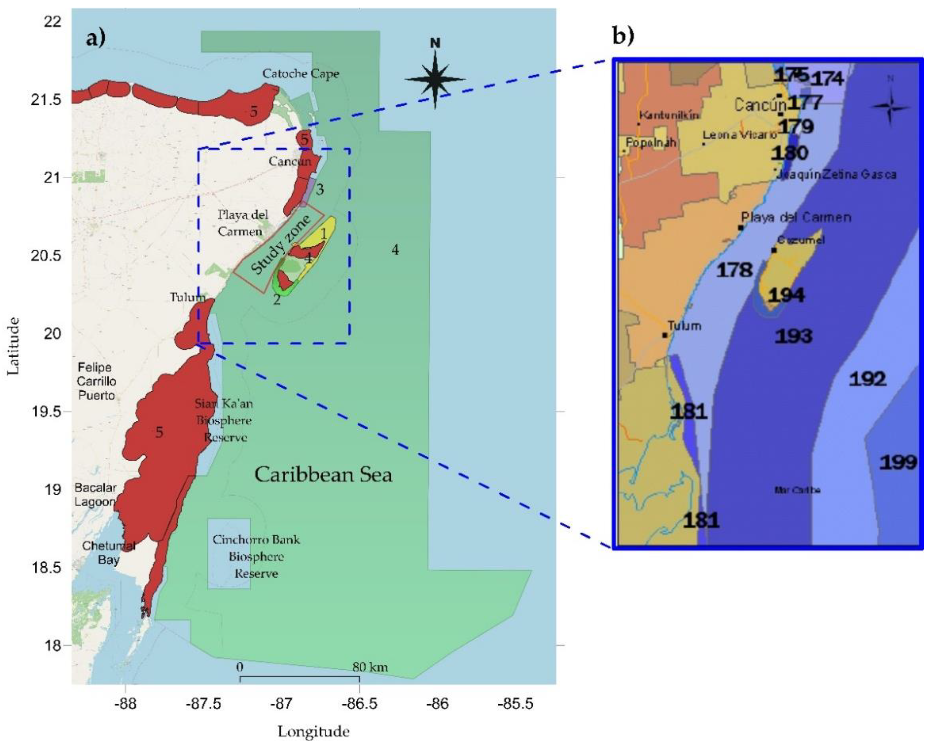
2.1.2. The Study Area

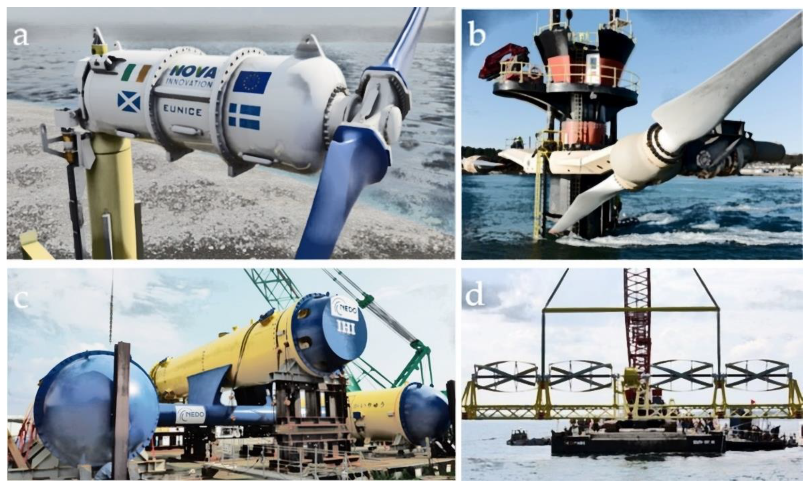
The area examined in this paper is the Cozumel channel (shown as a red polygon in Figure 1a,b), off the east coast of the Yucatan peninsula, 90 km SW of Cancun, between the island of Cozumel and Playa del Carmen. The main town on the island is also called Cozumel, located on the west coast (Figure 1c). Tourism is the main economic activity of the island and there is an international airport, a dock for cruise ships, and an hourly ferry connection to Playa del Carmen (Figure 1c).

The morphology of Cozumel Island is described fully in [43]; it lies 18 km in front of Playa del Carmen, Quintana Roo; has a maximum length of 53 km, SW-NE; and a width, NW-SE of 16 km in the centre (Figure 2). The island has an area of ~470 km² and a coastline of 124 km, mostly rocky. The west coast of the island has a narrower platform (500 to 1000 m to the −50 m isobath where the barrier reef begins). In this part of the island, there are three reef terraces at −5 m, −10 m, and −20 m. On the east coast, the insular platform is 1500 to 2500 m to −50 m, where the shelf edge begins, and there are five reef terraces at −3 m, −10 m, −20 m, −30 m, and −50 m, which are remnants of abrasion platforms from the Holocene era. The area of the northern platform is almost flat, at −20 to −30 m and ends at Arrowsmith Bank, about 50 km NNE of Cozumel (Figure 1). Figure 2 shows the bathymetry of the study area [44]. According to [45], ~5.05 Sv. (Sverdrups, equivalent to 10⁶ m³/s) passes through the channel.

Figure 3a shows a cross section of a bathymetric profile of the Cozumel channel. Figure 3b,c shows the bathymetric profile of each side of the channel [46]. On the Playa del Carmen side, the continental platform stretches less than a kilometre and the slope is very pronounced, ~68° (the green line in Figure 3b). On the other side of the channel (Figure 3c), the continental platform is 750 m in width, and the slope is ~29°. This is important when considering whether to install turbines on the sea bottom, in foundations or with anchors.

2.2. The Turbines

Although often ocean current turbines are often installed as arrays of devices, in this work, four individual commercial turbines were compared. (Figure 4). Two criteria were considered for the selection of the turbines. The first was that the stage of development of the devices is advanced, that is, at least at pre-commercial level. The second criteria was that there is information in the literature on the power curves, or sufficient data to estimate this, which is important as it allows comparisons between devices at sites previously identified as having hydrokinetic potential.

Of these turbines, there is the most information about the SeaGen and the NOVA, and the least information about the Kairyu. A brief description of the turbines is given, and summarized in Table 1. Three are axial turbines, with a horizontal axis of two blades, a cut in speed of 0.6–1 m/s, and nominal speeds of 1.5–2.2 m/s.

• The NOVA M100-D turbine (100 kW), Figure 4a, was developed by NOVA INNOVATION Ltd., UK [47]. It has a direct drive technology, using a simple rugged low-speed generator to directly convert the rotation of the blade into electricity. The rotor is 8.5 m in diameter and its nominal power is 100 kW at 2 m/s. The rotor is bi-directional. The system is fixed by gravity onto the seabed, so it does not require anchors or drilling.
• The Sea Gen turbine (1.2 MW), Figure 4b [48], was developed by Marine Current Turbines Ltd., now called Atlantis, UK. A prototype using this turbine was installed in 2008, but it is currently out of service. It had two 600 kW turbines working at ~2.5 m/s current speed, with two 16-meter diameter rotors. It lies on the seabed, needing foundations that require drilling.
• The Kairyu (100 kW), Figure 4c [49], is a floating turbine system. It generates ~100 kW at ~1.5 m/s. It is still at pre-commercial stage and is being developed by IHI Co., New Energy and Industrial Technology Development Organization (NEDO), Japan.
• The TidGen (150 kW), Figure 4d [50], was developed by Ocean Renewable Power Company ORPC, USA, and has four helical-type cross flow turbines, coupled to a single generator. Because of its elongated shape, it works well at shallow sites. At present, it is being considered for a tidal power project in Cobscook Bay, Maine, USA. It lies on the seabed and does not require anchors or drilling.

Figure 4. The hydrokinetic devices selected for the techno-econmic analysis: (a) NOVA M100-D turbine, with permission of [51]. (b) Sea Gen turbine, adapted from [52]. (c) Kairyu turbine, adapted from [49]. (d) TidGen turbine, with permission of [50].

Figure 4. The hydrokinetic devices selected for the techno-econmic analysis: (a) NOVA M100-D turbine, with permission of [51]. (b) Sea Gen turbine, adapted from [52]. (c) Kairyu turbine, adapted from [49]. (d) TidGen turbine, with permission of [50].

Table 1. Technical specifications of the turbines considered in this study.

	Sea Gen i	NOVA ii	Kairyu iii	TidGen iv
Nominal power (kW)	1200	100	100	150
Type	HATT *	HATT *	Horizontal axial	Cross flow
Number of turbines	2	1	2	4
Paddles	2	2	2	N/A
Diameter	18	8.5	11	5.1
Area	508	56.7	96.0	149.9
Specific power (kW/m2)	2.36	1.76	1.04	Est., 1
Cut-in speed	1	0.6	Est., 0.8	Est., 1.0
Nominal velocity (Approx.)	2.2	1.51	1.5	1.6
Lifetime (years)	11	20	N/A	N/A
Mounting	Seabed Pile-mounted	Seabed Bottom-mounted	Submerged Tethered	Seabed Bottom-mounted
Operation depth	N/A	20–25	30–50	18–45
Estimated Cost (M USD) Public CAPEX	16 v	3.74 vi	9.25 vii	1.2 viii
Investment cost USD/kW	13,333	37,400	92,500	8000

CAPEX = Capital Expenditure in Million U.S. dollars. * HATT = Horizontal Axial Tidal Turbine. ⁱ From [53]. ⁱⁱ [51]. ⁱⁱⁱ [54]. ^iv [55]. ^v [48], ^vi From [51], ^vii [49]/Data year 2019, ^viii [56]/data year 2010.

Table 1. Technical specifications of the turbines considered in this study.

	Sea Gen i	NOVA ii	Kairyu iii	TidGen iv
Nominal power (kW)	1200	100	100	150
Type	HATT *	HATT *	Horizontal axial	Cross flow
Number of turbines	2	1	2	4
Paddles	2	2	2	N/A
Diameter	18	8.5	11	5.1
Area	508	56.7	96.0	149.9
Specific power (kW/m2)	2.36	1.76	1.04	Est., 1
Cut-in speed	1	0.6	Est., 0.8	Est., 1.0
Nominal velocity (Approx.)	2.2	1.51	1.5	1.6
Lifetime (years)	11	20	N/A	N/A
Mounting	Seabed Pile-mounted	Seabed Bottom-mounted	Submerged Tethered	Seabed Bottom-mounted
Operation depth	N/A	20–25	30–50	18–45
Estimated Cost (M USD) Public CAPEX	16 v	3.74 vi	9.25 vii	1.2 viii
Investment cost USD/kW	13,333	37,400	92,500	8000

CAPEX = Capital Expenditure in Million U.S. dollars. * HATT = Horizontal Axial Tidal Turbine. ⁱ From [53]. ⁱⁱ [51]. ⁱⁱⁱ [54]. ^iv [55]. ^v [48], ^vi From [51], ^vii [49]/Data year 2019, ^viii [56]/data year 2010.

2.3. Methods of Estimating Potential Power

2.3.1. Simulated Data for the Estimation of Available Power

The estimated current velocities at the nodes in the channel were obtained from simulations using the HYCOM model (HYbrid Coordinate Ocean Model) [8]. Simulations using this model give predictions for the velocity components with a periodicity of 3 h and are distributed through a web repository accessed with the OPeNDAP protocol [57].

The database used was the Global Ocean Forecasting System 3.1 [58], which has records from July 2014. In this study (Figure 5), data was taken from the web repository from July 2014 to December 2019, for the geographic coordinates of the study area and the desired time range.

The data were obtained in Network Common Data Form (netCDF) format and were restructured to build a probability distribution of the current velocity at all available nodes in the study area. The data extraction, transformation, and loading process were carried out using the R programming language and the ncdf4 library [59].

The sea water velocities (in m/s), eastward sea water velocity at a depth z; (u_z), northward sea water velocity at a depth z; and (v_z), at depths (z) of 0–50 m [0, 2, 4, 6, 8, 10, 12, 15, 20, 25, 30, 35, 40, 45, 50], were used. For the analysis, the results of both components U = (u² + v²)^0.5 were calculated for all the depths mentioned above, where U is the resultant velocity, u is the eastward component, and v is the northward component, all in m/s.

Figure 5 shows the bathymetry of the study area and the nodes analysed. As can be seen, most of these nodes are at depths of <100 m. In Figure 5, the measurement sites used by [40] were included (see Sites (a), (b) and (c)).

In that study, Acoustic Doppler Current Profilers (ADCPs), attached to a buoy at 130 m depth, were used providing useful data from 22 to 121 m water depths. These measurements were taken from August 2002–August 2003 along the Mexican Caribbean coast.

2.3.2. Potential Hydrokinetic Estimates and Theoretical Use

To compare the theoretical energy harvested by the device with the potential hydrokinetic energy available, the mean annual power density in MWh/m²-year [37] was used. Equation (1) was applied to the velocity data for each node, (See Appendix A), to obtain the hydrokinetic energy (in MWh/m²-year) as the current passes the shallowest 50 m of the total water depth. With these values, an average theoretical energy potential was obtained for depths of 0–50 m [0, 2, 4, 6, 8, 10, 12, 15, 20, 25, 30, 35, 40, 45, 50].

Equation (3), presented by [60], was reformulated and then applied to obtain the energy generated by the turbines in specified operational site conditions. This type of calculation, applied to marine turbines, is described by [9], who considers it necessary to have the following data:

• The energy potential available at a given site (latitude, length and depth, period of time (Appendix A,

  Table A1. Example of the Organization of Data for Each Node and Depth, Node 1.

  Node Location				Velocity Range (m/s)																				Σ
  Node	lat	lon	Std Depth	0.1	0.2	0.3	0.4	0.5	0.6	0.7	0.8	0.9	1	1.1	1.2	1.3	1.4	1.5	1.6	1.7	1.8	1.9	<2
  	Degres	Degres	m	Hours in Each Velocity Range																				h/year
  1	20.32	−87.12	0	1	17	124	259	527	982	1556	2022	1868	1019	327	53	6	1	1	0	0	0	0	0	8760
  1	20.32	−87.12	2	1	7	96	241	490	1010	1594	2156	1915	937	269	38	4	1	0	0	0	0	0	0	8760
  1	20.32	−87.12	4	1	2	94	238	481	1029	1610	2223	1927	890	231	31	3	0	0	0	0	0	0	0	8760
  1	20.32	−87.12	6	1	1	93	234	471	1055	1668	2299	1898	819	197	23	2	0	0	0	0	0	0	0	8760
  1	20.32	−87.12	8	0	2	93	230	476	1090	1748	2393	1811	737	156	20	2	0	0	0	0	0	0	0	8760
  1	20.32	−87.12	10	0	2	94	227	480	1132	1812	2443	1767	663	122	16	1	0	0	0	0	0	0	0	8760
  1	20.32	−87.12	12	0	4	95	229	490	1177	1893	2465	1703	597	95	11	1	0	0	0	0	0	0	0	8760
  1	20.32	−87.12	15	0	4	94	228	521	1258	1989	2516	1610	468	66	4	1	0	0	0	0	0	0	0	8760
  1	20.32	−87.12	20	1	7	99	236	610	1422	2114	2557	1377	297	38	3	0	0	0	0	0	0	0	0	8760
  1	20.32	−87.12	25	1	13	109	263	734	1569	2330	2443	1081	198	16	2	0	0	0	0	0	0	0	0	8760
  1	20.32	−87.12	30	1	22	127	319	881	1723	2504	2242	804	126	11	1	0	0	0	0	0	0	0	0	8760
  1	20.32	−87.12	35	1	38	127	376	1046	1851	2630	1994	601	87	7	1	0	0	0	0	0	0	0	0	8760
  1	20.32	−87.12	40	1	65	121	433	1188	1997	2729	1730	460	34	3	1	0	0	0	0	0	0	0	0	8760
  1	20.32	−87.12	45	1	66	118	490	1305	2179	2791	1489	303	17	1	0	0	0	0	0	0	0	0	0	8760
  1	20.32	−87.12	50	1	59	124	542	1462	2455	2776	1171	162	8	1	0	0	0	0	0	0	0	0	0	8760

  ).
• The electrical output power curve (Appendix A,

  Table A2. Total Efficiency Curves (%) for Each Technology.

  	Velocity of Ocean Current (m/s)
  Turbines	0.1	0.2	0.3	0.4	0.5	0.6	0.7	0.8	0.9	1	1.1	1.2	1.3	1.4	1.5	1.6	1.7	1.80	1.90	2.00	2.10
  	η(U)
  SeaGen 1	0.00	0.00	0.00	0.00	0.20	0.27	0.35	0.43	0.40	0.40	0.40	0.40	0.42	0.45	0.41	0.42	0.44	0.40	0.42	0.43	0.36
  Nova 2	0.00	0.00	0.00	0.00	0.00	0.07	0.15	0.23	0.33	0.42	0.44	0.47	0.46	0.46	0.43	0.39	0.36	0.28	0.22	0.17	0.14
  Kairyu 3	0.00	0.00	0.00	0.00	0.00	0.00	0.00	0.00	0.43	0.55	0.55	0.55	0.49	0.43	0.31	0.27	0.24	0.18	0.14	0.11	0.09
  TidGen 4	0.00	0.00	0.00	0.00	0.00	0.00	0.00	0.00	0.15	0.19	0.20	0.21	0.21	0.22	0.16	0.14	0.12	0.09	0.07	0.06	0.05

  ¹ Adapted from [53]; ² Adapted from [51]; ³ Adapted from [54]; ⁴ Adapted from [55].

  ) considers the cut-in and cut-out velocities. This is the power curve, which is a function of the design characteristics of the turbine, such as the power coefficient (C_p), turbine subsystems (e.g., the gearbox), generator conversion efficiency, and other energy losses. In this work, the resulting marine hydrokinetic energy for the site of interest in a certain time is considered as the theoretical power estimation approach.
• It was also assumed that in the case of seabed-based technologies such as SeaGen, Nova, and TidGen, the evaluation of their performance is based on a floating type of installation.

Considering the approach of [37], the energy density in terms of a period of 1 hour (E in Wh/m²) in a defined period of time (T) is given by Equation (1).

$$E={\int }_0^{\mathrm{T}}Pdt$$

(1)

$$P=\frac{1}{2}\mathsf{\rho }{U}^3$$

(2)

where P is the power density (W/m²) of the marine current (Equation (2)), U is the speed of current (m/s), and $\mathsf{\rho }$ is the sea-water density (kg/m³). To compare the energy generated by each device, the MWh/m²-year was used, i.e., the energy extracted by the device, theoretically, from the hydrokinetic potential available at each node (Equation (3)). Subsequently, this value was multiplied by the area of the selected turbine, shown in Figure 4, giving the total energy generated in a year, in MWh/year; in other words, the technical power availability for each turbine.

$$P_e\left(\mathrm{z},\mathrm{n}\right)=\frac{1}{2}\mathsf{\rho }A{\displaystyle \sum }_{u_i\in U}{\left(H_{yr}\right)}_{u_i}\eta \left(u_i\right)u_i^3$$

(3)

where P_e (z,n) represents the estimated production of electrical energy for every HYCOM node, n, and for every depth value, z ∈{0,2,4,6,8,10,12,15,20,25,30,35,40,45,50 in meters}. The values of P_e (z,n) were evaluated from the distribution over the time of speed of the marine current, (U, in m/s). This distribution is represented by ${\left(H_{yr}\right)}_{u_i}$, the mean number of hours per year when the speed had estimated values in the interval $\left[u_i-0.05,u_i+0.05\right]$, for $u_i\in U=\left\{0.05,0.15,0.25,\dots ,1.85,1.95\right\}$ (Appendix A). The total efficiency of the system (for each turbine) can be expressed as η(U) = C_pη_g, (Appendix A), where, C_p is the power coefficient of the turbine; and η_g is the efficiency of the electricity generator and the generator turbine coupling. Therefore, the turbinate flow is directly related to the speed. For the calculations, the density $\mathsf{\rho }$ = 1023, 78 kg/m³ at 26 °C, 36 PSU and one atmosphere of pressure [61] were considered; A is the cross-sectional area of the turbine in perpendicular contact with the flow of the current (in m²). With the electrical production values of each turbine, for the different depths in each node, an average of 0–50 m of depth was obtained (in MWh/year).

To spatially represent the theoretical power estimation (Figure 6), QGIS was used: 3.10.2-A Coruña with the triangulated Irregular Interpolation (TIN) algorithm with the Clough-Toucher interpolation methodology [62]. The spatial extension was from longitude −87.34844°, latitude 20.205527°, to longitude −86.64844°, latitude 20.89669°, with an output raster size of 200 rows and a height of 204 columns. To obtain the layout over the Cozumel channel, a blanking continuous action map was made using 32 nodes with values of 0.001 MWh/m²-year. The nodes were selected 16 on each side of the channel, along the coasts.

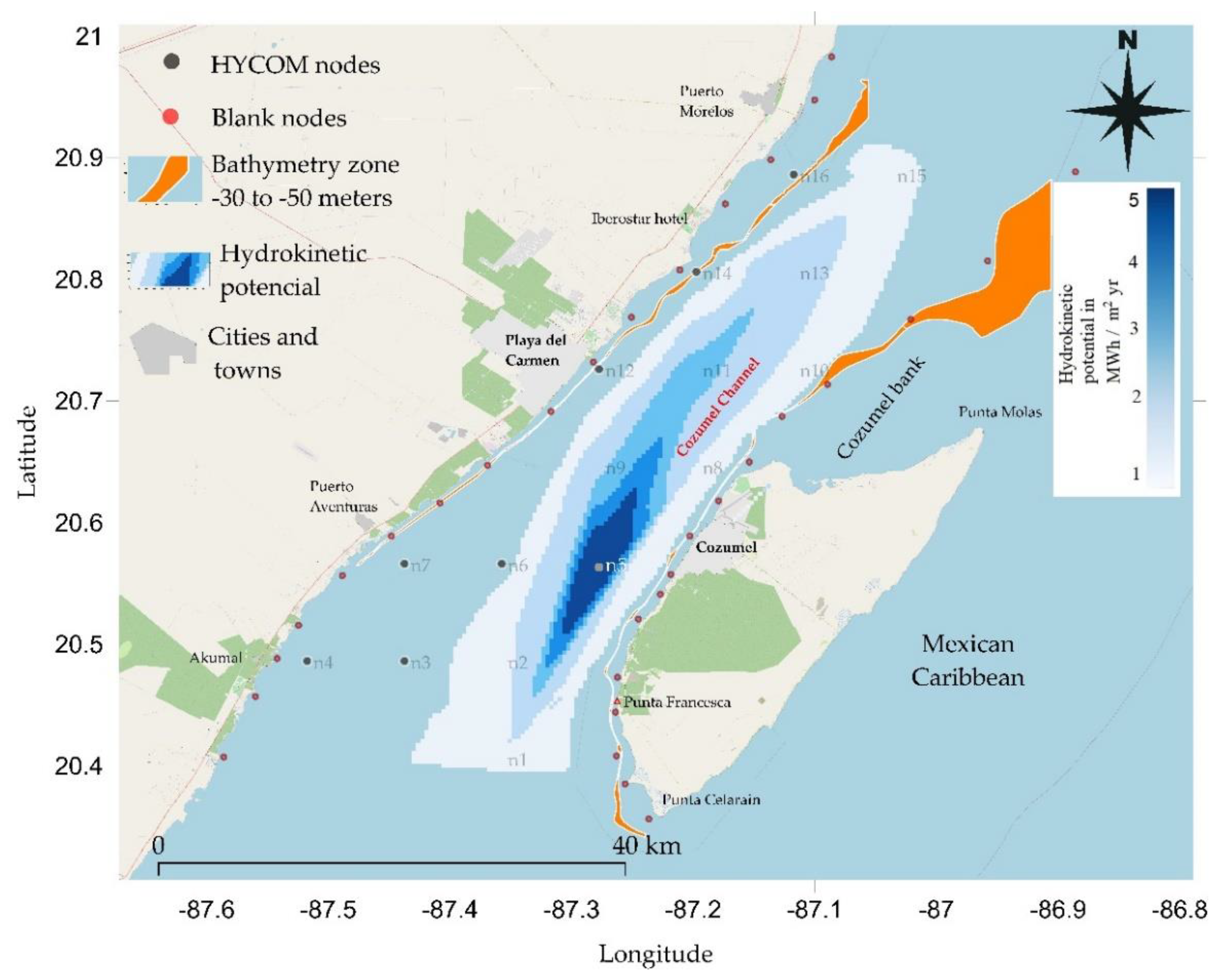
2.3.3. Delimitation of the Most Suitable Area

Three criteria were used to identify which areas have the most potential for this type of energy generation.

• First, whether the device would be floating or placed on the seabed. As seen in Table 1, it is suggested that for floating devices, their anchors are no deeper than 100 m [54], while for water depths <50 m, it is recommended that the devices rest on the seabed.
• The second criterion is the average hydrokinetic potential generated per year obtained with Equation (1).
• Thirdly, social and environmental constraints that would restrict installation or manoeuvring at the energy use site must be taken into account.

The results of the first two criteria suggest that the best sites for floating technology would be between the −30 m and −100 m isobaths, while for technology resting on the seabed, optimal sites would be between the −30 and −50 m isobaths. For these conditions, the height of the turbines, seen in Table 1, and the bathymetric charts of the Mexican Navy [63] were taken into account (YE. 922.1, S. M. 922.4) as well as the Bathymetric Chart of the IBCCA (sheet 1-06) [44].

To meet the needs of the third criteria, areas which have restrictions regarding maritime traffic; protected natural areas [64]; strategic infrastructure, such as cables for electricity or telecommunications; and sites close to airports, military zones, and research centres, must be excluded from the study. All these restrictive elements should be documented on maps and web pages of the relevant agencies, such as the Secretariat of the Mexican Navy [65], the Secretariat of Communications and Transportation [66], and the Secretariat of Energy [67].

Figure 6. Energy field from analysis of the HYCOM data. The orange area is between 30 to 50 m depth. Data from [65].

Figure 6. Energy field from analysis of the HYCOM data. The orange area is between 30 to 50 m depth. Data from [65].

2.4. Estimating Energy Costs

In order to compare the cost of the energy produced by each of the devices, the methodology of [68] was used to obtain LCOE estimates for the various ocean technologies. The LCOE is the sum of the initial investment cost, plus operational costs, divided by the production of energy during the useful life of the system. This methodology defines the parameters of capital expenditures (CAPEX), operating and maintenance expenses (OPEX), and input resource data.

As it is expected that the LCOE for the deployment of the first array will prove uncompetitive, the LCOE was applied for a project with a minimum installed capacity of 0.3 MW, CAPEX of $ 5100/kW, and OPEX of $ 160/kW-year, and a maximum installed capacity of 10 MW with CAPEX of $ 14,600/kW and OPEX of $ 1160/kW-year.

$$\mathrm{LCOE}=\frac{\mathrm{CAPEX}+{{\displaystyle \sum }}_t^n\frac{\mathrm{OPEX}}{{\left(1+r\right)}^t}}{{{\displaystyle \sum }}_t^n\frac{\mathrm{AEP}}{{\left(1+r\right)}^t}}$$

(4)

CAPEX is the capital expenditure, and OPEX is the operational expenditure (for year t), AEP is the annual electricity production (at year t), r is the discount rate, n is the lifetime of the system, and t is the year from the start of project. CAPEX includes both fixed and variable investment costs such as planning, manufacturing, and construction. The OES [68] recommends a discount rate r of 8.5 to 12.5% and t of 20 years.

The C.F., expressed by Equation (5), is the Capacity Factor, which is the ratio of energy actually produced by an energy generating unit or system, in a given period T (8760 h per year), compared to the hypothetical maximum. This can be expressed as a percentage (over a given reference period) or as full load hours per year. AEP is the total energy produced by the system during a year in MWh/year or kWh/year. $\overline{P}$ is the nominal power of the turbine in kW or MW [69].

$$\mathrm{C}.\mathrm{F}.=\frac{\mathrm{AEP}}{\overline{P}·\mathrm{T}}$$

(5)

The CAPEX value was estimated for each device as [60].

$$\mathrm{CAPEX}=\frac{C_i}{{\lambda }_i}$$

(6)

In Equation (6), the costs in C_i (in USD) are the generator, rotor, coupling, installation (cable; network connection, and foundations), and their participation percentages λ_i. The percentage of each category was calculated depending on the characteristics of each device with the mathematical models of [60].

2.5. Methods for Evaluating Environmental and Social Restrictions

Any project that would affect coastal, marine, or jungle ecosystems in the study area must be discussed in a process of public consultation [70]. Therefore, regulations for the protected natural areas (PNA) [64] and the ecological management programs in the study area were reviewed [71]. With this information, descriptive maps of the study area were made, showing the area that can potentially be impacted.

Parallel to these environmental criteria, the parts of the study area described as strategic were also mapped: (a) power transmission lines and power plants; (b) the airports, cabotage ports, shipping routes, and military zones; (c) areas with important economic activities, mainly tourism; and (d) any areas with major infrastructure, such as roads or towns. The mapping was done using the geo portal of the National Commission for the Knowledge and Use of Biodiversity [72], and the bathymetric charts of the Secretariat of the Navy [63], information from the Federal Electricity Commission (CFE), and the National Commission of Natural Protected Areas (CONANP),

To organize this information, free software QGIS 3.10, 64 Bit, WGS 84, Windows 10, under General Public License [62] was used. And Google Earth Pro 7.3.3.7786 (64-bit), Microsoft Windows Operating System (6.2.9200.0) from © 2020 Google LLC, was used to produce georeferenced KML information [73]. To adapt the figures, © 1993-2012 Golden Software Inc, Surfer version 11.0.642 (64-bit) Surface Mapping System [74] was also used.

3. Results of the Technical Analysis

3.1. Estimating Power Availability

Figure 6 shows the average hydrokinetic potential per year for each node shown in Figure 5, from the sea surface to a depth of −50 m (MWh/m²-year). The values range from 0.0075 MWh/m²-year to 6 MWh/m²-year for nodes 4 and node 5, respectively. It can be seen that the area with greatest potential is 6–7 km off the Cozumel coast, where the channel depth is over 400 m (Figure 2), in front of Punta Francesca and Punta Langosta.

The areas with depths of −30 to −50 m, which could be used for devices based on the seabed, have low hydrokinetic energy potential, around 1 MWh/m²-year. Even for floating devices anchored at −100 m or less, the potential is only 2 MWh/m²-year (Figure 6).

3.2. Reference Data Results

Table 2. The hydrokinetic potential in the study area.

Location	Long	Lat	Distance to the Coast	Mean Hidrokinetic Energy Potential	Mean Direction	Standard Deviation	Source
	Degrees	Degrees	km	MWh/m2-year	Degrees	Degrees
Puerto Morelos	−86.751	20.841	12	9.85	45	1.3	Data from [40]
Cozumel east coast	−86.751	20.841	8	3.27	51	0.4
Tulum	−87.138	20.079	17	1.54	79	0.4

shows the hydrokinetic potential for the reference sites of [40], as well as the average direction of the current and its standard deviation. Based on these data, the site with greatest potential is site (a), in the Cozumel Canal, followed by sites (b) and (c), which are shown in Figure 5.

In the case of site (a), the measurements reported by [40] are close to those for Node 15 using HYCOM. The HYCOM hydrokinetic potential (Figure 6) is around 2 MWh/m²-year; about five times less than the 9.85 MWh/m²-year obtained using the data reported by [40].

3.3. Technical Availability and Potential Sites

Table 3. Theoretical energy extracted in 1 year per turbine, at −30 to −50 m depth, per node and per device in MWh/year using Equation (3).

Turbine	1	2	3	4	5	6	7	8	9	10	11	12	13	14	15	16
Sea Gen	381	392	37	0	1319	121	0	380	600	334	660	29	563	38	234	6
Nova	28	29	1	0	151	5	0	30	58	24	66	0	54	1	16	0
Kairyu	37	41	0	0	269	0	0	45	108	32	123	0	99	0	21	0
TidGen	9	8	0	0	65	0	0	9	23	6	26	0	21	0	4	0

shows the theoretical energy extracted in 1 year for the four turbines considered in this analysis. The MWh/year values at each of the 16 nodes are reported. The HYCOM nodes used to evaluate the energy potential were 5, 9, 11, and 13. These results indicate that SeaGen uses 40% of the energy potential, Kairyu 39%, Nova 36.4%, and TidGen 5.5%.

3.4. Capacity Factor

Table 4. Average Capacity Factor at 0 to −50 m depth, for each node, for the four turbines.

	Capacity Factor (in %) of Each Device and at Each Node
Device	1	2	3	4	5	6	7	8	9	10	11	12	13	14	15	16
Sea Gen	3.6	3.7	0.4	0.0	12.5	1.1	0.0	3.6	5.7	3.2	6.3	0.28	5.36	0.36	2.228	0.05
Nova	3.2	3.4	0.1	0.0	17.3	0.5	0.0	3.4	6.7	2.7	7.6	0.04	6.19	0.08	1.829	0.00
Kairyu	4.2	4.7	0.0	0.0	30.7	0.0	0.0	5.1	12.3	3.7	14.0	0.00	11.25	0.00	2.421	0.00
TidGen	1.0	0.9	0.0	0.0	7.4	0.0	0.0	1.0	2.6	0.7	3.0	0.00	2.35	0.00	0.490	0.00

shows the average capacity factors (in percentages) calculated for each node and the four turbines. The capacity factors (Table 4) for each device were located for the best site, which was node 5 (Figure 5). The device with the highest plant factor was the Karyu with almost 31%.

4. Results of the Economic Analysis

4.1. Investment Costs for Each Device

Table 5. Comparison of public and calculated LCOE.

Device	1 Public CAPEX	Ranc CAPEX 2		Calculated CAPEX 3
	USD/kW	Min USD/kW	Max USD/kW	USD/kW
Sea Gen	12,500	5100	14,600	5985
Nova	37,400			22,959
Kairyu	92,500			24,615
TidGen	8000			16,501

¹ The Public cost is from official web pages of the turbine manufacturers, data from Table 1. ² Ranc CAPEX is First array/First Project (Note: “expected to be installed between 2020 and 2030, are not the long-term cost reduction target”) [68]. ³ Calculated with [68]. The international CAPEX was provided by Ocean Energy Systems.

shows the Public CAPEX (cost from official web pages of the turbine manufacturers) and the calculated CAPEX (obtained using the methodology of [68]) compared with the Ranc CAPEX (first array/first project) of [68]. The most expensive devices are Nova and Kairyu. SeaGen and TidGen have more competitive Public and Calculated CAPEX.

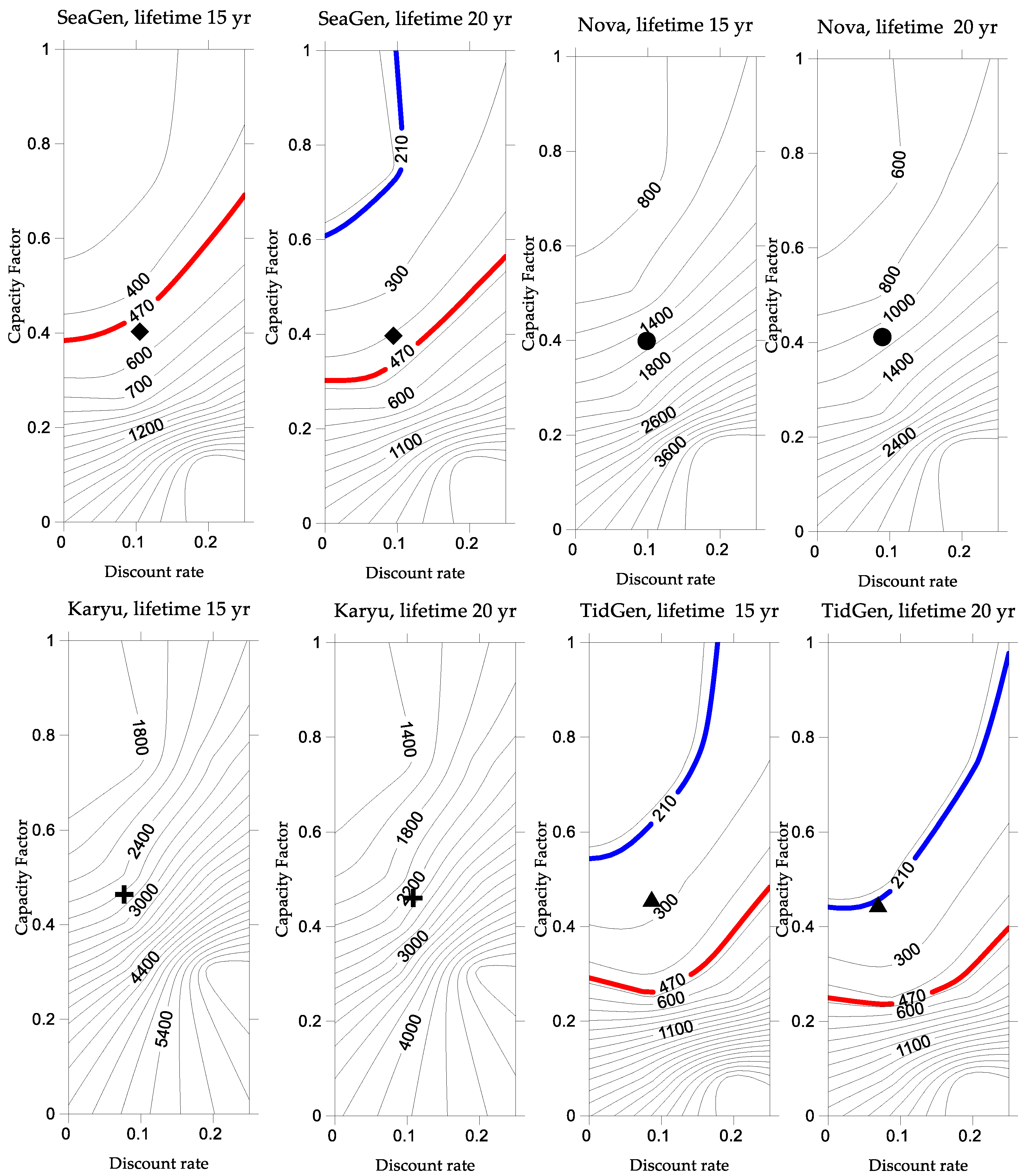
4.2. Levelised Cost of Energy

Table 6. LCOE for the turbines using the maximum Capacity Factor at node 5.

Device	Public LCOE 5	Ranc LCOE 6		Calculated LCOE 7
	USD/MWh	Min USD/MWh	Max USD/MWh	USD/MWh
Sea Gen 1	N/A	210	470	1148
Nova 2	N/A			2264
Kairyu 3	N/A			4012
TidGen 4	N/A			1673

¹ CF = 12.5%, ² CF = 17.3%, ³ CF = 30.7%, ⁴ CF = 7.4%. Values of Table 5 Capacity Factor for Node 5. ^1,2,3,4 Lifetime of the installation 20 years, discount rate r = 0.085, and value of CAPEX public in Table 6. OPEX 160 USD/kW·Yr. ⁵ The Public cost is from official web pages of the turbines corporations, data from Table 1. ⁶ Reference LCOE is for Second array/Second Project in tidal technology [68]. ⁷ Calculated with [68] and the Public CAPEX Table 5. The international CAPEX was provided by Ocean Energy Systems.

shows the levelised cost of energy (LCOE) for the devices evaluated, for node 5, which is the best location in terms of the energy potential available, using HYCOM data. In the table it can be seen that there are no public LCOEs available. However, an LCOE calculated with the methodology of [68] is shown. Comparing the referenced LCOE of [68], it is seen that these are well above the international references of 210–470 USD/MWh for a second for tidal technology project, as no LCOE references for ocean current technology exist as of yet. The reason for these high values is the low Capacity Factors of the four devices, as three were designed for marine conditions not found in the Cozumel channel.

To offer a more competitive LCOE, possible scenarios of LCOE estimated with the public CAPEX of each device are included in Figure 7, which describes scenarios for the four turbines, considering two lifetimes (15 and 20 years), and varying discount rates (r) from 0 to 0.25, and Capacity Factors of 0 to 1. It is seen that the high costs of the NOVA and Kairyu devices give high LCOE costs that are not within the LCOE reference for tidal technology, 5100 USD/kW to 14,600 USD/kW (Table 5 and Table 6). The SeaGen device does attain the LCOE reference values of [68], only when the energy potential is 2500 W/m² (21.9 MWh/m²-year), but the closest value in the area is the one obtained with data from ADCP [40] of 9.85 MWh/m²-year. The best scenario was found for a lifetime of 20 years, with a low discount rate of around 0.1, Capacity Factor of at least 0.4, and CAPEX of less than 15,000 USD/kW.

5. Challenges

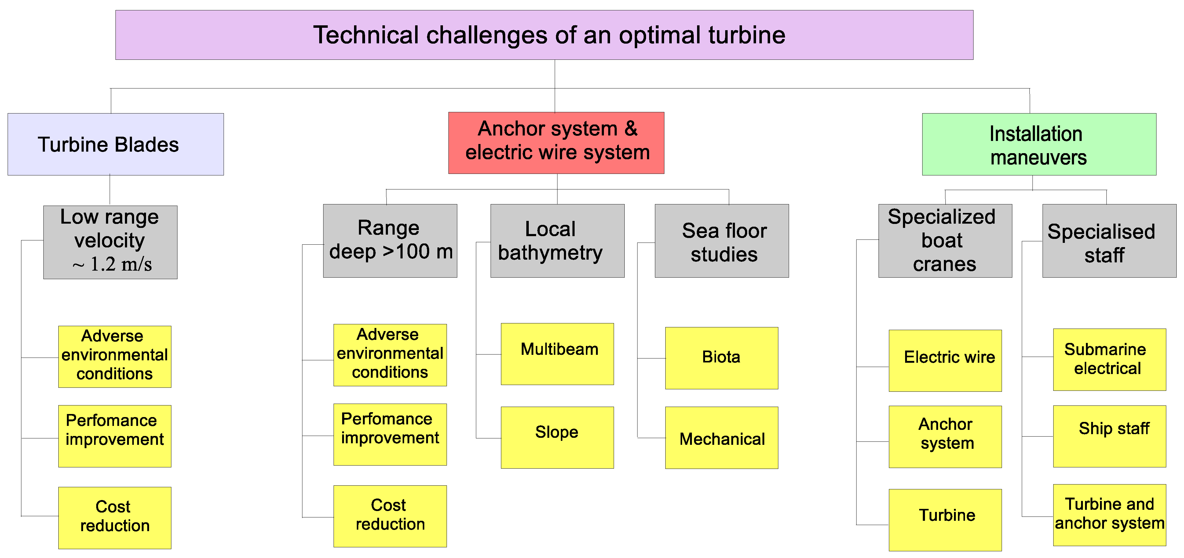
5.1. Technical Challenges for the Optimal Turbine

From the results of obtained in the previous section and the literature reviewed, it is seen that there are challenges that had not been previously identified, related to the installation of turbines in the Cozumel channel. The tree diagram presented in Figure 8 shows the technical challenges to be faced, if we are to better take advantage of the energy potential of this area.

One of the greatest technical constraints is that the highest energy potentials are found at depths of around 400 m. Another important challenge is the design of the turbine blades, which must be capable of taking advantage of the hydrokinetic potential at low speeds. In addition, the difficulties involved in installing a device in an area with a unidirectional current, and waves with a different direction, are very challenging.

Design of the turbine blades. It was found that the designs analysed in this work make poor use of the energy potential in the Cozumel channel. Energy generation cannot be defined only by the cut-in speed, but also by the energy conversion efficiency curve of each device. The turbine that takes most advantage of the current is the Kairyu with a Capacity Factor of 30.7%, which means that a turbine design more suited to the Yucatan Current would significantly increase the Capacity Factor. On the other hand, the design of these turbines must allow the turbine to survive storms, hurricanes, and biological fouling. In all the above assessments, low investment and operation costs are prioritized, (Figure 7), yielding an investment cost of <12,500 USD/kW (Table 5) even with a Capacity Factor (CF) of 0.5 resulting in an LCOE < 470 USD/MWh.

The anchoring system. As reported by [51], the depth range for the anchoring system for floating or bed-based devices is 20 to 30 m, because these systems are placed in shallow channels where the current is intensified by the effects of the tides. Only one system was designed for ocean currents: the Kuroshio current, in Japan. This floating device operates at 30–50 m depth, although it may be anchored at up to 100 m depth. In the Cozumel channel, the best sites are in areas with depths of around 400 m, with potentials in the first 50 m depth of up to 6 MWh/m²-year. Areas with depths of less than 100 m have almost 1 MWh/m²-year. For these water depths, the anchoring system presents a serious challenge. Regarding the possible use of depths between 30 and 50 m deep, Muckelbauer [43] mentions that on the terraces of the channel, which are up to 50 m deep, there are various coral, sponge, algae, and sea grass species, therefore, special measures are needed to avoid affecting these ecosystems.

Connection to the electric grid. Electric transmission lines must be installed from the seabed, either above or below ground. This could impact on the areas of reef or seagrass. Also the associated electromagnetic fields could pose a risk for the orientation of some species [75,76,77].

Installation logistics. As the highest energy potentials are found at depths of around 400 m, it is important to consider the complications involved in installing devices at this depth, since both the availability of vessels, and qualified personnel for them, is of the utmost importance.

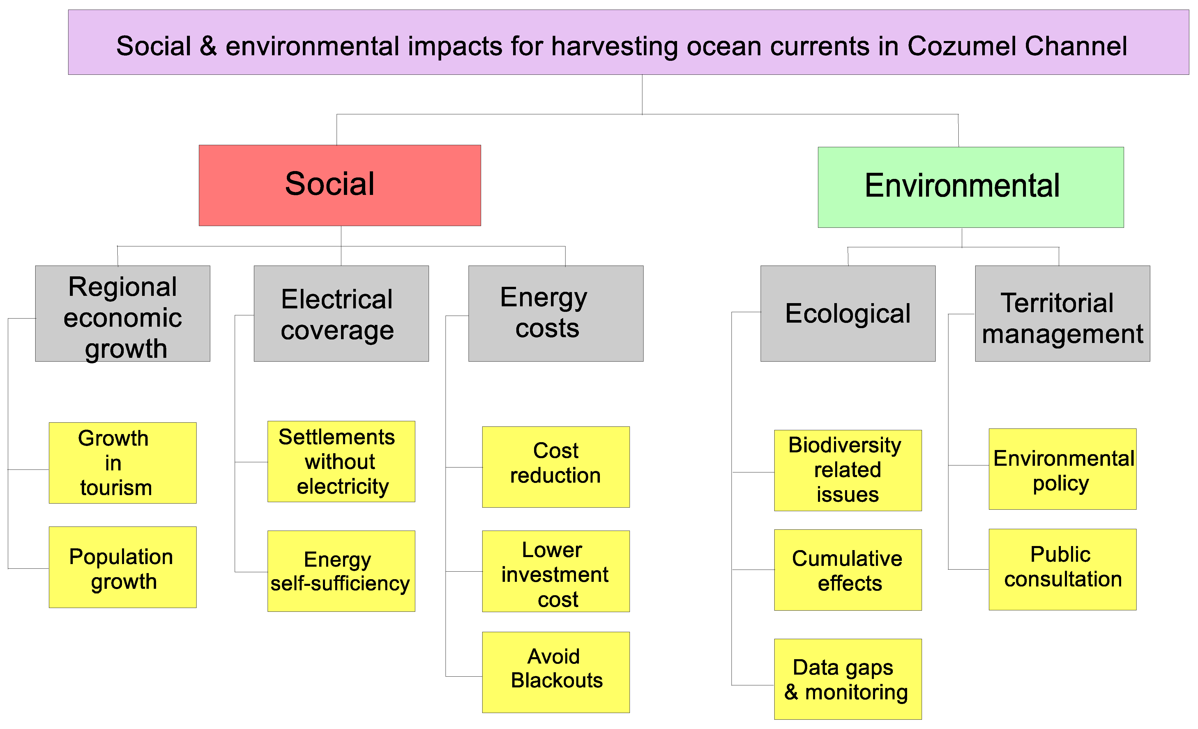
5.2. Social and Environmental Impacts

Figure 9 shows social and environmental impacts that hydrokinetic energy harvesting in Cozumel may occasion, considering the various processes involved. Public consultation is one of the most critical factors regarding environmental impact statements. Existing environmental restrictions are also decisive in decision making.

Protected areas. In the study area, there are four Protected Natural Areas (PNAs), the largest of which covers the entire Mexican Caribbean, and is shown in green in Figure 10a. The other PNAs around Cozumel island are shown in Figure 10a: the northern portion and the eastern, terrestrial, and marine coastal strip of the island of Cozumel (number 1); Cozumel reefs (number 2); and close to the study area are the Puerto Morelos reefs (number 3) [64]. In addition, the mangrove areas are priority sites (Number 5) [72].

Ecological management programs. The study area has two ecological ordering programs, one regional that includes the Gulf of Mexico and another local that depends on the State of Quintana Roo:

• The Marine and Regional Ecological Planning Program for the Gulf of Mexico and the Caribbean Sea [71] provides guidance on the use of natural resources and the development of productive activities. It identifies, guides, and links the policies, programs, projects, and actions of the public administration that contribute to achieving the regional goals set, and to optimizing the use of public resources (Figure 10b).
• The Ecological Zoning Programs of the State of Quintana Roo are made up of nine Local Ecological Zoning Programs for which the Ministry of Ecology and Environment is responsible. [78].

Protected species in the area. Some species in the area are protected by NOM-059-SEMARNAT-2010 [79]. This covers the protection of native Mexican species of flora and fauna, including those at risk.

Maritime transit. Two trans-Caribbean companies [80]: Ultramar passengers [81] and Ultramar Carga, [82] operate in the area. For passengers, ferries run from Playa del Carmen to Cozumel, and for cargo from Punta Venado Calica to Cozumel, running regularly throughout the day, 7 days a week. Cruisers also use the Cozumel Channel, arriving at the Maritime Cruise Terminal, at Punta Langosta on Cozumel, from the north, and leaving from the same direction (Figure 11).

Infrastructure. Restrictions as to the feasibility of operating a marine turbine facility include the underwater cables that would take electricity to Cozumel from the substations in Playa del Carmen. There is also the international airport on the island of Cozumel (CZM) and two airways, one on Cozumel, and another in Playa del Carmen, used for local air transport (Figure 11). The cruise ship dock and the local ferry and cargo ports could also impede the development of a marine turbine facility project (Figure 11).

Tourist areas. The tourist zone of this area is called the Riviera Maya, which includes the towns of Puerto Morelos, Playa del Carmen, Puerto Aventuras, Akumal, Tulum, Cobá, and the Sian Ka’an Reserve. The study area only includes the first two (Figure 10). The island of Cozumel is also important for tourism, including the towns of Cozumel and El Cedral, and the coastal areas of the island, used mainly for tourism activities (Figure 11).

Research facilities. There are several research centres in the area, such as the Institute of Marine Sciences and Limnology (ICMyL) and the Academic Unit of Reef Systems (UASA) of the National Autonomous University of Mexico (UNAM), which has a monitoring system for meteorological and oceanographic parameters, called the Academic Meteorological and Oceanographic Monitoring Service (SAMMO). This centre is in Puerto Morelos (Figure 6), as is the Regional Centre for Fisheries Research (CRIP), which works on the lobster Panulirus argus, shrimp, queen conch larvae Lobatos gigas, sharks, and rays, and also has a coral nursery and carries out coral restoration [83].

Military installations. There is a Military Air Base on the same site as the Cozumel International Airport (CZM), as well as the Cozumel Naval Sector, next to the cruise ship dock in Punta Langosta Isla (Figure 11).

Considering these social and environmental restrictions, three areas seem to offer the most possibilities for the installation of a marine turbine park (Figure 11).

Table 7. Area in the Cozumel Channel.

Zone	Area (km2)	Areas Vertices
A	60	−87.0436, 20.5276	−87.007, 20.5012	−87.0933, 20.4337	−87.06181, 20.41159
B	10	−86.9952, 20.5837	−86.9730, 20.5473	−86.9646, 20.5666	−87.0032, 20.5685
C	20	−86.96285, 20.65161	−86.95320, 20.59284	−86.93344, 20.63027	−86.986938, 20.610492

shows areas vertices of the promising areas delineated in Figure 11. These three areas could be enlarged or reduced, depending on the results of more specific studies.

In Area A (Figure 11), a simple arrangement of axial turbines, spaced at a lateral distance equal to the diameter of the turbine, would accommodate around 150 SeaGen turbines, for maximum theoretical electricity production: 150 turbines × 1319 MWh/year = 197 GWh/year. In the case of the Nova device, this value would be 323 Nova turbines = 48 GWh/year; while for Kairyu device, 90 Kairyu turbines = 24 GWh/year.

In Areas B and C, with similar theoretical energy extracted in 1 year (Figure 11) and for the same number of turbines for each device, the maximum theoretical electricity production is ~100 GWh/year for SeaGen. For Nova, this value would be ~21 GWh/year, and for Kairyu ~11 GWh/year.

6. Conclusions

Of the 16 potential sites analysed, that with highest energy potential was Node 5 (Latitude 20.48; Longitude –87.04) with <6 MWh/m²-year, equivalent to an average of <685 W/m². This energy potential is for the uppermost 50 m of the water column. At this depth, there are no energy-generating devices operating at present, so it will be a challenge to harness these energy potentials at depths of over 100 m.

Of the four types of devices evaluated, none is wholly perfect for the site conditions, mainly because of the depth of the Cozumel channel, around 400 m. The device most suitable for the area is that designed to take advantage of the Kuroshio current, off Japan, the Kairyu turbine. This floating device can operate at a maximum depth of 50 m, but has an anchoring system for a depth of up to 100 m. However, this device was seen to have one of the highest investment costs in the economic analysis performed.

Since the devices evaluated were designed for other speed ranges, we limited the Capacity Factor to reduce the LCOE. This is something that could be explored in future research. If a specific turbine design could be developed to use more of the hydrokinetic energy available, for the speeds in the study area, the Plant Factor and technical feasibility could be increased.

In a theoretical scenario, the SeaGen has the most competitive LCOE, at 564.3 USD/MWh, with a Capacity Factor of 50% for 15 years and r = 0.2. The LCOE was 342.8 USD/MWh, for a Capacity Factor of 50%, for 20 years and r = 0.125. In general, the best scenario for every device was for a lifetime of 20 years, with a low discount rate of around 0.1, Capacity Factor of at least 0.4, and a CAPEX value of less than 15,000 USD/kW.

Sites previously identified by other authors as having good potential are nodes 9, 11, and 13, with an energy density in the order of 3–4 MWh/m²-year. For example, research in the Cozumel channel area mentions power densities in the order of 1.54 MWh/m²-year to 4.48 MWh/m²-year, [6]. Alcérreca-Huerta et al. [17] reported values of 2.63–8.76 MWh/m²-year, although using the data from [40], values up to 9.85 MWh/m²-year were obtained. Similarly, at Cape Hatteras, values of 8.76–6.92 MWh/m²-year were found [9]. All these power densities refer to ocean currents, and not tides.

This paper describes an initial technical evaluation showing a theoretical annual electricity production of 197 GWh/year using a 150 SeaGen turbine, which is 4.37% of the 2017 total electricity consumption of Quintana Roo. However, 197 GWh/year is more than all the energy generated from Turbogas technology in the state that year. The energy balance for Quintana Roo is positive, at 86 GWh/year. It is estimated that for every Turbogas plant in Quintana Roo, the equivalent of 50,000 tons of CO₂ would be saved (0.454 tonnes of CO₂/MWh) [84], giving an annual saving of the equivalent of 88,650 tons of CO₂ emissions.

References

1. Gross, R.; Leach, M.; Bauen, A. Progress in Renewable Energy. Environ. Int. 2003, 29, 105–122. [Google Scholar] [CrossRef]
2. Hussain, A.; Arif, S.M.; Aslam, M. Emerging Renewable and Sustainable Energy Technologies: State of the Art. Renew. Sustain. Energy Rev. 2017, 71, 12–28. [Google Scholar] [CrossRef]
3. Halkos, G.E.; Gkampoura, E.-C. Reviewing Usage, Potentials, and Limitations of Renewable Energy Sources. Energies 2020, 13, 2906. [Google Scholar] [CrossRef]
4. Roy, A.; Auger, F.; Dupriez-Robin, F.; Bourguet, S.; Tran, Q.T. Electrical Power Supply of Remote Maritime Areas: A Review of Hybrid Systems Based on Marine Renewable Energies. Energies 2018, 11, 1904. [Google Scholar] [CrossRef] [Green Version]
5. Tomabechi, K. Energy Resources in the Future. Energies 2010, 3, 686–695. [Google Scholar] [CrossRef] [Green Version]
6. Hernández-Fontes, J.V.; Felix, A.; Mendoza, E.; Cueto, Y.R.; Silva, R. On the Marine Energy Resources of Mexico. J. Mar. Sci. Eng. 2019, 7, 191. [Google Scholar] [CrossRef] [Green Version]
7. Quitoras, M.R.D.; Abundo, M.L.S.; Danao, L.A.M. A Techno-Economic Assessment of Wave Energy Resources in the Philippines. Renew. Sustain. Energy Rev. 2018, 88, 68–81. [Google Scholar] [CrossRef]
8. Chassignet, E.P.; Hurlburt, H.E.; Metzger, E.J.; Smedstad, O.M.; Cummings, J.A.; Halliwell, G.R.; Bleck, R.; Baraille, R.; Wallcraft, A.J.; Lozano, C.; et al. Global Ocean Prediction with the Hybrid Coordinate Ocean Model (HYCOM). Oceanography 2009, 22, 13. [Google Scholar] [CrossRef]
9. Bane, J.M.; He, R.; Muglia, M.; Lowcher, C.F.; Gong, Y.; Haines, S.M. Marine Hydrokinetic Energy from Western Boundary Currents. Annu. Rev. Mar. Sci. 2017, 9, 105–123. [Google Scholar] [CrossRef] [Green Version]
10. Gründlingh, M.L. On the Course of the Agulhas Current. S. Afr. Geogr. J. 1983, 65, 49–57. [Google Scholar] [CrossRef]
11. Lutjeharms, J.R. The Agulhas Current; Springer: Berlin, Germany, 2006; Volume 329. [Google Scholar]
12. Barkley, R. The Kuroshio Current. Sci. J. 1970, 6, 54–60. [Google Scholar]
13. Sawada, K.; Handa, N. Variability of the Path of the Kuroshio Ocean Current over the Past 25,000 Years. Nature 1998, 392, 592–595. [Google Scholar] [CrossRef]
14. Fofonoff, N. The Gulf Stream. In Evolution of Physical Oceanography: Scientific Surveys in Honor of Henry Stommel; Warren, B.A., Wunsch, C., Eds.; MIT Press: Cambridge, MA, USA, 1981; pp. 112–139. [Google Scholar]
15. Stommel, H.M. The Gulf Stream: A Physical and Dynamical Description; University of California Press: Berkeley, CA, USA, 1965. [Google Scholar]
16. Davis, B.; Farrel, J.; Swan, D.; Jeffers, K. Generation of Electrical Power from the Florida Current of the Gulf Stream. In Proceedings of the Offshore Technology Conference, Houston, TX, USA, 5–8 May 1986. [Google Scholar]
17. Alcérreca-Huerta, J.C.; Encarnacion, J.I.; Ordoñez-Sánchez, S.; Callejas-Jiménez, M.; Gallegos Diez Barroso, G.; Allmark, M.; Mariño-Tapia, I.; Silva Casarín, R.; O’Doherty, T.; Johnstone, C.; et al. Energy Yield Assessment from Ocean Currents in the Insular Shelf of Cozumel Island. JMSE 2019, 7, 147. [Google Scholar] [CrossRef] [Green Version]
18. Marais, E.; Chowdhury, S.; Chowdhury, S. Theoretical Resource Assessment of Marine Current Energy in the Agulhas Current along South Africa’s East Coast. In Proceedings of the 2011 IEEE Power and Energy Society General Meeting, Detroit, MI, USA, 24–28 July 2011; pp. 1–8. [Google Scholar]
19. Meyer, I.; Van Niekerk, J.L. Towards a Practical Resource Assessment of the Extractable Energy in the Agulhas Ocean Current. Int. J. Mar. Energy 2016, 16, 116–132. [Google Scholar] [CrossRef]
20. Wright, S.; Chowdhury, S.; Chowdhury, S. A Feasibility Study for Marine Energy Extraction from the Agulhas Current. In Proceedings of the 2011 IEEE Power and Energy Society General Meeting, Detroit, MI, USA, 24–28 July 2011; pp. 1–9. [Google Scholar]
21. Moodley, R.; Nthontho, M.; Chowdhury, S.; Chowdhury, S. A Technical and Economic Analysis of Energy Extraction from the Agulhas Current on the East Coast of South Africa. In Proceedings of the 2012 IEEE Power and Energy Society General Meeting, San Diego, CA, USA, 22–26 July 2012; pp. 1–8. [Google Scholar]
22. Chang, M.-H.; Tang, T.Y.; Ho, C.-R.; Chao, S.-Y. Kuroshio-Induced Wake in the Lee of Green Island off Taiwan. J. Geophys. Res. Ocean. 2013, 118, 1508–1519. [Google Scholar] [CrossRef]
23. Hsu, T.-W.; Liau, J.-M.; Liang, S.-J.; Tzang, S.-Y.; Doong, D.-J. Assessment of Kuroshio Current Power Test Site of Green Island, Taiwan. Renew. Energy 2015, 81, 853–863. [Google Scholar] [CrossRef]
24. Kiyomatsu, K.; Kodaira, T.; Kadomoto, Y.; Waseda, T.; Takagi, K. Adcp Measurements of Ocean Currents near Miyake Island. J. Jpn. Soc. Nav. Archit. Ocean Eng. 2014, 20. [Google Scholar] [CrossRef] [Green Version]
25. Kodaira, T.; Waseda, T.; Nakagawa, T.; Isoguchi, O.; Miyazawa, Y. Measuring the Kuroshio Current around Miyake Island, a Potential Site for Ocean-Current Power Generation. Int. J. Offshore Polar Eng. 2013, 23, 272–278. [Google Scholar]
26. Liu, T.; Wang, B.; Hirose, N.; Yamashiro, T.; Yamada, H. High-Resolution Modeling of the Kuroshio Current Power South of Japan. J. Ocean Eng. Mar. Energy 2018, 4, 37–55. [Google Scholar] [CrossRef]
27. Webb, A.; Waseda, T.; Kiyomatsu, K. A High-Resolution, Long-Term Wave Resource Assessment of Japan with Wave–Current Effects. Renew. Energy 2020, 161, 1341–1358. [Google Scholar] [CrossRef]
28. Chen, F. Kuroshio Power Plant Development Plan. Renew. Sustain. Energy Rev. 2010, 14, 2655–2668. [Google Scholar] [CrossRef]
29. VanSwieten, J.H.; Meyer, I.; Alsenas, G.M. Evaluation of Hycom as a Tool for Ocean Current Energy Assessment. In Proceedings of the 2nd Marine Energy Technology Symposium METS14, Seattle, WA, USA, 15–18 April 2014; p. 11. [Google Scholar]
30. Yang, X.; Haas, K.A.; Fritz, H.M. Evaluating the Potential for Energy Extraction from Turbines in the Gulf Stream System. Renew. Energy 2014, 72, 12–21. [Google Scholar] [CrossRef] [Green Version]
31. Yang, X.; Haas, K.A.; Fritz, H.M. Theoretical Assessment of Ocean Current Energy Potential for the Gulf Stream System. Mar. Technol. Soc. J. 2013, 47, 101–112. [Google Scholar] [CrossRef]
32. Duerr, A.; Dhanak, M. Hydrokinetic Power Resource Assessment of the Florida Current. In Proceedings of the OCEANS 2010 MTS/IEEE SEATTLE, Seattle, WA, USA, 20–23 September 2010; pp. 1–7. [Google Scholar]
33. Duerr, A.E.; Dhanak, M.R. An Assessment of the Hydrokinetic Energy Resource of the Florida Current. IEEE J. Ocean. Eng. 2012, 37, 281–293. [Google Scholar] [CrossRef]
34. Kang, D.; Curchitser, E.N.; Rosati, A. Seasonal Variability of the Gulf Stream Kinetic Energy. J. Phys. Oceanogr. 2016, 46, 1189–1207. [Google Scholar] [CrossRef]
35. Kabir, A.; Lemongo-Tchamba, I.; Fernandez, A. An Assessment of Available Ocean Current Hydrokinetic Energy near the North Carolina Shore. Renew. Energy 2015, 80, 301–307. [Google Scholar] [CrossRef]
36. Encarnacion, J.I.; Johnstone, C.; Ordonez-Sanchez, S. Design of a Horizontal Axis Tidal Turbine for Less Energetic Current Velocity Profiles. J. Mar. Sci. Eng. 2019, 7, 197. [Google Scholar] [CrossRef] [Green Version]
37. Byun, D.S.; Hart, D.E.; Jeong, W.J. Tidal Current Energy Resources off the South and West Coasts of Korea: Preliminary Observation-Derived Estimates. Energies 2013, 6, 566–578. [Google Scholar] [CrossRef]
38. Nim IV, C. The Political Ecology of Environmental Change and Tourist Development in Cozumel, Mexico. Ph.D. Thesis, Miami University, Oxford, OH, USA, 2006. [Google Scholar]
39. Hernández-Fontes, J.V.; Martínez, M.L.; Wojtarowski, A.; González-Mendoza, J.L.; Landgrave, R.; Silva, R. Is Ocean Energy an Alternative in Developing Regions? A Case Study in Michoacan, Mexico. J. Clean. Prod. 2020, 266, 121984. [Google Scholar] [CrossRef]
40. Cetina, P.; Candela, J.; Sheinbaum, J.; Ochoa, J.; Badan, A. Circulation along the Mexican Caribbean Coast. J. Geophys. Res. Ocean. 2006, 111. [Google Scholar] [CrossRef] [Green Version]
41. Secretaría de Energía Dirección General de Planeación e Información Energéticas Sistema de Información Energética. Available online: http://sie.energia.gob.mx/ (accessed on 29 March 2021).
42. Centro Nacional de Control de Energía. Programa de Desarrollo del Sistema Electrico Nacional 2018–2032; Secretaría de Energía: Mexico City, México, 2018; p. 330. [Google Scholar]
43. Muckelbauer, G. The Shelf of Cozumel, Mexico: Topography and Organisms. Facies 1990, 23, 201–239. [Google Scholar] [CrossRef]
44. Instituto Nacional de Estadística y Geografía International Bathymetric Chart of the Caribbean Sea and the Gulf of Mexico, Chart 1-06. 2018. Available online: https://www.ngdc.noaa.gov/mgg/ibcca/ib_start.htm (accessed on 29 March 2021).
45. Chávez, G.; Candela, J.; Ochoa, J. Subinertial Flows and Transports in Cozumel Channel. J. Geophys. Res. Ocean. 2003, 108. [Google Scholar] [CrossRef]
46. Secretaría de Marina. S.M. 922.1 Costa Este, Isla Mujeres a Isla Cozumel; Secretaría de Marina: Mexico City, Mexico, 2003. [Google Scholar]
47. Nova-Innovation Tidal Turbines: Nova M100-D. Available online: https://www.novainnovation.com/tidalturbines (accessed on 11 July 2020).
48. Power-Technology SeaGen Turbine, Northern Ireland. Available online: https://www.power-technology.com/projects/strangford-lough/ (accessed on 2 August 2020).
49. Nikkei Electricity from Ocean Currents: Japanese Company to Begin Experiment (Photo Credits by Annu Nishioka). Available online: https://asia.nikkei.com/Spotlight/Environment/Electricity-from-ocean-currents-Japanese-company-to-begin-experiment (accessed on 25 May 2020).
50. ECO. ORPC Ireland Selected for Major Ocean Energy Project (Photo Credits by ORCP). Available online: https://www.ecomagazine.com/news/industry/orpc-ireland-selected-for-major-ocean-energy-project (accessed on 13 April 2020).
51. Innovation, N. Products—Nova Innovation. Available online: https://www.novainnovation.com/products/ (accessed on 29 March 2021).
52. Scottish-Energy-News Major Boost for Scottish Tidal Energy Industry as Atlantis Takes over of Siemens’ UK Marine-Power Subsidiary (Photo Credits by Siemens AG). Available online: http://www.scottishenergynews.com/major-boost-for-scottish-wave-energy-industry-as-atlantis-takes-over-of-siemens-uk-marine-power-subsidiary/ (accessed on 11 July 2020).
53. Boehme, T.; Taylor, J.; Wallace, R.; Bialek, J. Matching Renewable Electricity Generation With Demand; Academic Study; The University of Edinburgh: Edinburgh, Scotland, 2006; p. 77. [Google Scholar]
54. IHI Corporation Power Generation Using the Kuroshio Current. IHI Eng. Rev. 2014, 46, 4.
55. Ocean Renewable Power Company TidGen Power System. Available online: https://www.orpc.co/our-solutions/scalable-grid-integrated-systems/tidgen-power-system (accessed on 29 March 2021).
56. VanZwieten, J.; McAnally, W.; Ahmad, J.; Davis, T.; Martin, J.; Bevelhimer, M.; Cribbs, A.; Lippert, R.; Hudon, T.; Trudeau, M. In-Stream Hydrokinetic Power: Review and Appraisal. J. Energy Eng. 2014, 141, 16. [Google Scholar] [CrossRef]
57. OPeNDAPTM. Advanced Software for Remote Data Retrieval. Available online: https://www.opendap.org/ (accessed on 30 March 2021).
58. HYCOM Consortium HYCOM Data Server. Available online: https://www.hycom.org/dataserver (accessed on 30 March 2021).
59. Pierce, D. Ncdf4: Interface to Unidata NetCDF; RCoreTeam: Vienna, Austria, 2019. [Google Scholar]
60. Vazquez, A.; Iglesias, G. Capital Costs in Tidal Stream Energy Projects–A Spatial Approach. Energy 2016, 107, 215–226. [Google Scholar] [CrossRef] [Green Version]
61. IOC; SCOR; IAPSO. The International Thermodynamic Equation of Seawater—2010. Calculation and Use of Thermodynamic Properties. Intergovernmental Oceanographic Commission, Manuals and Guides No. 56, UNESCO (English). 2010, p. 196. Available online: http://www.teos-10.org/pubs/TEOS-10_Manual.pdf (accessed on 30 March 2021).
62. QGIS Project 23.1.5. Interpolación—Documentación de QGIS Documentation. Available online: https://docs.qgis.org/3.10/es/docs/user_manual/processing_algs/qgis/interpolation.html?highlight=tin#tin-interpolation (accessed on 30 March 2021).
63. Secretaría-de-Marina. Catálogo de Cartas y Publicaciones Náuticas; Secretaría-de-Marina: Mexico City, Mexico, 2021; p. 25, Nautical Chart S.M. 922., S. M. 922.1, S. M. 922.2, S. M. 922.3, S. M. 922.4, S. M. 922.5, S. M. 922.6 y S. M. 922.7. 2021. [Google Scholar]
64. Comisión Nacional de Áreas Naturales Protegidas Información espacial de las Áreas Naturales Protegidas CONANP. Available online: http://sig.conanp.gob.mx/website/pagsig/info_kml.htm (accessed on 30 March 2021).
65. Secretaría de Marina. S.M. 922-4, Isla de Cozumel Q Roo; Secretaría de Marina: Mexico City, Mexico, 2010. [Google Scholar]
66. Secretaría de Comunicaciones y Transporte Informe Estadístico Mensual. Movimiento de Carga, Buques y Pasajeros En Los Puerto de México. Available online: https://www.gob.mx/sct (accessed on 31 March 2021).
67. Secretaría de Energía. Centro Nacional de Control de Energía Programa de Ampliación y Modernización de la Red Nacional de Trasmisión y Redes Generales de Distribución del Mercado Eléctrico Mayorista, PRODESEN 2019–2033; Secretaría de Energía: Mexico City, México, 2019; p. 576. [Google Scholar]
68. Ocean Energy Systems International Levelised Cost Of Energy for Ocean Energy Technologies, An Analysis of the Development Pathway and Levelised Cost of Energy Trajectories of Wave, Tidal and OTEC Technologies. Available online: https://www.ocean-energy-systems.org/documents/65931-cost-of-energy-for-ocean-energy-technologies-may-2015-final.pdf/ (accessed on 31 March 2021).
69. Wave Energy Centre; Co-ordinated Action of Ocean Energy EU funded Project (CA-OE); Implementing Agreement on Ocean Energy Systems (IEA-OES). Ocean Energy Glossary; Ocean Energy Systems: Lisbon, Portugal, 2007; p. 14. [Google Scholar]
70. IFT. Instituto de Federal de Telecomunicaciones IFT Portal de Internet. Available online: www.ift.org.mx (accessed on 7 November 2020).
71. Secretarias de Gobernación, Diario Oficial de la Federación ACUERDO Por El Que Se Expide La Parte Marina Del Programa de Ordenamiento Ecológico Marino y Regional Del Golfo de México y Mar Caribe y Se Da a Conocer La Parte Regional Del Propio Programa (Continúa En La Segunda Sección). Available online: http://dof.gob.mx/nota_detalle_popup.php?codigo=5279084 (accessed on 18 March 2021).
72. Comisión Nacional de Áreas Naturales Protegidas Portal de Información Geográfica—CONABIO. Available online: http://www.conabio.gob.mx/informacion/gis/?vns=gis_root/biodiv/monmang/bimagstipr/sitpriogw (accessed on 12 March 2021).
73. Google Google Earth Pro. Available online: https://www.google.com/intl/es/earth/download/gep/agree.html (accessed on 30 March 2021).
74. Golden Software. Inc Full User’s Guide Golden Software, Inc.; Golden Software: Golden, CO, USA, 2012. [Google Scholar]
75. Copping, A.; Hanna, L.; Whiting, J.; Geerlofs, S.; Grear, M.; Blake, K.; Coffey, A.; Massaua, M.; Brown-Saracino, J.; Battey, H. Environmental Effects of Marine Energy Development around the World Annex IV Final Report; Ocean Energy Systems: Lisbon, Portugal, 2013; p. 96. [Google Scholar]
76. Martínez, M.L.; Vázquez, G.; Pérez-Maqueo, O.; Silva, R.; Moreno-Casasola, P.; Mendoza-González, G.; López-Portillo, J.; MacGregor-Fors, I.; Heckel, G.; Hernández-Santana, J.R.; et al. A Systematic View of Potential Environmental Impacts of Ocean Energy Production. Renew. Sustain. Energy Rev. 2021, 149, 111332. [Google Scholar] [CrossRef]
77. Wiltschko, W.; Wiltschko, R. Magnetic Orientation and Magnetoreception in Birds and Other Animals. J. Comp. Physiol. A 2005, 191, 675–693. [Google Scholar] [CrossRef]
78. Secretaría de Ecología y Medio Ambiente Ordenamiento Ecológico, Secretaría de Ecología y Medio Ambiente, Del Estado de Quintana Roo. Available online: http://sema.qroo.gob.mx/bitacora/index.php/ordenamiento-ecologico (accessed on 24 May 2021).
79. Secretaría de Medio Ambiente y Recursos Naturales. NORMA Oficial Mexicana NOM-059-SEMARNAT-2010, Protección Ambiental-Especies Nativas de México de Flora Y Fauna Silvestres-Categorías de Riesgo Y Especificaciones Para Su Inclusión, Exclusión o cambio-Lista de Especies En Riesgo; Secretaría de Medio Ambiente y Recursos Naturales: Mexico City, Mexico, 2010; Volume NOM-059-SEMARNAT-2010, p. 78. [Google Scholar]
80. Naviera M29 Transcaribe, Naviera M29. Available online: https://transcaribe.net/ (accessed on 30 March 2021).
81. Ultramar Ultramar, Rutas y Horarios, Ferry Pasajeros. Available online: https://www.ultramarferry.com/es/rutas-y-horarios (accessed on 30 March 2021).
82. Ultramar Carga Ultramar Carga—Experience Innovation. Available online: http://ultramarcarga.com/ (accessed on 30 March 2021).
83. Instituto Nacional de Pesca Acciones y Programas. Available online: https://www.gob.mx/inapesca (accessed on 31 March 2021).
84. Subsecretaría de Planeación y Política Ambiental; Dirección General de Políticas para el Cambio Climático. AVISO. Para El Reporte del Registro Nacional de Emisiones; SEMARNAT: México City, Mexico, 2015; p. 1. [Google Scholar]
Figure 1. (a) The Peninsula of Yucatán, Mexico. (b) The study area, shown by the red polygon. (c) Aerial view from the NW coast of Cozumel island.
Energies 14 04411 g001
Figure 2. Bathymetry of the Cozumel channel. Isobaths show meters. The transect A–B shows the line of the bathymetric profile seen in Figure 3.
Energies 14 04411 g002
Figure 3. (a) The Cozumel channel (~1/45) at its narrowest width, ~18 km, between Playa del Carmen and the town of Cozumel. (b) The coast off Playa del Carmen; (c) The coast off Cozumel.
Energies 14 04411 g003
Figure 5. Bathymetric view of the Cozumel channel. Taken from sheet 1-06 from [44]. The red line shows the study area, in which 16 HYCOM nodes (n1 to n16) are plotted. Sites (a), (b) and (c) are those evaluated by [40].
Energies 14 04411 g005
Figure 7. Theoretical representation of LCOE (USD/MWh) scenarios for the turbines, considering two lifetimes (15 and 20 years), and varying discount rates (r) from 0 to 0.25, and the Capacity Factor from 0 to 1. The public CAPEX and OPEX values were used. The maximum and minimum international LCOE value is shown in the blue and red lines, respectively [68]. The symbols rhombus ⯁, circle ⬤, cross ✚, and triangle ▲ show the LCOE at a Capacity Factor of 0.4, at a discount rate of 0.1 and with public CAPEX, respectively.
Energies 14 04411 g007
Figure 8. Diversity of technical challenges to be solved in order to have a suitable technology for the conditions of the Yucatan Current.
Energies 14 04411 g008
Figure 9. Social and environmental impacts from using the ocean currents in the Cozumel Channel to generate electricity through hydrokinetic devices.
Energies 14 04411 g009
Figure 10. (a) Protected Natural Areas and priority sites. (b) Environmental Management Unit (UGA) 178 in which the study area is located [71].
Energies 14 04411 g010
Figure 11. Maritime traffic and submarine cables that could restrict the use of marine currents. Sites A, B, and C have the fewest restrictions of an environmental or social nature. Sources: (Secretary of the Navy, 2010), (Conabio, 2020), (Open-Sea-Map, 2020).
Energies 14 04411 g011