A Novel Method for Structural Lightweight Design with Topology Optimization

Abstract

Topological optimization is an innovative method to realize the lightweight design. This paper proposes a hybrid topology optimization method that combines the SIMP (solid isotropic material with penalization) method and genetic algorithm (GA), called the SIMP-GA method. In the method, SIMP is used to update the chromosomes, which can accelerate convergence. The filtering scheme in the SIMP method can filter unconnected elements to ensure the connectivity of the structure. We studied the influence of varying the filtering radius on the optimized structure. Simultaneously, in the SIMP-GA method, each element is regarded as a gene, which controls the population number to a certain extent, reduces the amount of calculation, and improves the calculation efficiency. The calculation of some typical examples proves that the SIMP-GA method can obtain a better solution than the gradient-based method. Compared with the conventional genetic algorithm and GA-BESO (Bi-directional Evolutionary Structural Optimization) method, the calculation efficiency of the proposed method is higher and similar results are obtained. The innovative topology optimization method could be an effective way for structural lightweight design.

1. Introduction

With the development of society, in some specific fields, structural lightweight design is the most effective way to improve technical indicators, such as aerospace, automobiles, ships, bridges, and other construction industries. With the development of computer technology, structural optimization, especially structural topology optimization, is increasingly used in these fields to improve structural lightweight design.

Topological optimization is an innovative structural optimization method that can find an optimal material layout under specified conditions rapidly. In addition, it is of great significance for guiding structural design to realize the lightweight design. The main methods used include homogenization [1], SIMP [2,3,4], ESO (evolutionary structural optimization) [5,6,7,8] and level set [9,10,11] methods. Simultaneously, genetic algorithms [12,13] are also constantly developing and are gradually being applied in topology optimization [14].

Since the publication of Bendsoe and Kikuchi [1], the topology optimization for continuum structure has been investigated extensively. However, the homogenization-based approach adopted in many papers has the disadvantage that the determination and evaluation of optimal microstructures and their orientations are cumbersome if not unresolved (for noncompliance problems). Furthermore, the resulting structures cannot be built since there is no definite length-scale associated with the microstructures [15,16]. To reduce the complexity of the homogenization method, SIMP was proposed by Bendsoe [2]. The advantage of SIMP is that it can ignore the microstructure and uses a continuous fictitious isotropic material, the elasticity tensor of which is assumed to be a function of material density [17]. However, for both of the homogenization-based approaches and SIMP, the discrete design variable is relaxed and allowed to attain all values between 0 and 1 [17,18]. Therefore, the optimum structure may contain a great deal of intermediate material which is far from the 0–1 solution required. To make the structure close to the 0–1 design, the intermediate material should be penalized with the power law [19].

SIMP is a method of single-point search using sensitivity. While it has the advantage of high calculation efficiency, in general, it can only converge to the local optimal solution. By contrast, the genetic algorithm [12] is a multi-point search method that can find different local optimal solutions, and during the search process, new search points can be generated, allowing more local optimal solutions to be sought. However, the multi-point search of the genetic algorithm leads to a large increase in the amount of calculation. Due to limitations of computational cost, the genetic algorithm is mostly used for topology optimization of discrete truss systems [20], but it cannot handle large-scale finite elements in the optimization of continuum structures [21,22,23], so the topology results are not good.

Another major drawback of applying genetic algorithms to topology optimization is connectivity. Due to the randomness of genetic algorithms, isolated structures that appear in the optimization process are not connected to the overall structure, so there is no way to transfer loads. An isolated structure is meaningless. In their algorithm, Jackiela et al. [23] removed isolated structures by setting unconnected elements to invalid material. Fanjoy and Crossley [24] used chromosome masks to avoid isolated structures. When genetic algorithms are applied to the topology optimization of continuum structures, connectivity analysis is inevitable [21,22,23,24], but the method of handling connectivity is not very effective, and adds further computational costs.

In this context, the development of a method that combines the genetic algorithm and a gradient-based method is desirable. In the hybrid algorithm, the gradient information is used to screen and sort the population, which can ensure the connectivity of the structure. Liu X et al. [25] proposed the GESO method, combining the genetic algorithm and ESO method. In the GESO method, the structure is discretized with finite elements and each element is regarded as an individual. The conventional genetic algorithm applies the population globally at the structural level. Compared with the genetic algorithm alone, the GESO method reduces the calculation required. The main drawback of the GESO method comes from the ESO method, which can only delete elements. Therefore, Zuo et al. [26] proposed a GA-BEAO topology optimization method, combining the genetic algorithm and BESO method, the latter an improvement on the shortcomings of ESO. To solve the connectivity problem, the algorithm gradually punishes the probability of crossing and mutation to a certain maximum value. Chen et al. [27] proposed a method combining the optimality criteria (OC) method and genetic algorithm. In this method, OC were used to obtain the initial structure, after which the genetic algorithm was used to search for the optimal solution globally. Qu et al. [28] proposed an IGA-BESO topology optimization method that combines the improved genetic algorithm, which increases the calculation efficiency, and the BESO method.

Here, we propose a SIMP-GA method which combines the SIMP method with a genetic algorithm. In the method, each element is regarded as a gene in a chromosome, and all elements constitute an individual. A certain number of individuals are set to form a population for evolutionary operations such as crossover and mutation. This will not increase the population number as the size of the finite element becomes larger, so the calculation efficiency can be further improved. Furthermore, the chromosome is updated using SIMP, and its filtering technology is used to filter unconnected elements, thereby ensuring the connectivity of the structure. The results obtained by the SIMP-GA method are binary, so the intermediate density elements typically obtained by the SIMP method are avoided in the topology results.

In Section 2, the theoretical basis of the SIMP method and the related concepts of genetic algorithms are introduced. Section 3 details the implementation of the SIMP-GA method. Section 4 proposes several examples to verify the SIMP-GA method. Section 5 describes the validation results including the calculations and a detailed comparison among SIMP, BESO, GA-BESO and SIMP-GA. Section 6 is the conclusions.

2. Topology Optimization for Minimum Compliance Problem

2.1. SIMP Method

The general topology optimization problem is to find the optimal material distribution under certain constraints, such as a volume constraint, to minimize the objective function. Considering the maximum stiffness design and the fact that the strain energy density is easily integrated over the entire design domain, minimizing the compliance of the design is often chosen as the objective function.

Therefore, in most cases, the topology optimization problem is to minimize the compliance of a structure subject to a constraint on the volume of material used, which can be written as

$$\begin{array}{cc}\mathrm{Min}: & c\left(\mathit{x}\right)={\displaystyle \int \mathsf{\sigma }\mathrm{d}\epsilon \mathrm{dV}={\displaystyle {\sum }_{\mathrm{e}=1}^N{{\displaystyle \mathit{u}}}_{\mathrm{e}}^{\mathrm{T}}{{\displaystyle \mathit{k}}}_{\mathrm{e}}}}{{\displaystyle \mathit{u}}}_{\mathrm{e}}\\ & V\left(\mathit{x}\right)\le {{\displaystyle V}}_{\max }\\ \mathrm{Subject} \mathrm{to}: & \mathit{K}\mathit{U}=\mathit{F}\\ & {{\displaystyle \mathit{x}}}_{\min }\le \mathit{x}\le {{\displaystyle \mathit{x}}}_{\max }\end{array}$$

(1)

where $\mathit{U}$ and $\mathit{F}$ are the global displacement and force vectors, respectively; $\mathit{K}$ is the global stiffness matrix; ${\mathit{u}}_{\mathrm{e}}$ and ${\mathit{k}}_{\mathrm{e}}$ are the element displacement vector and stiffness matrix, respectively; $\mathit{x}$ is the vector of the design variables; ${\mathit{x}}_{\min }$ and ${\mathit{x}}_{\max }$ are the lower and upper limits of the design variables, respectively; $N=\left(nelx\times nely\right)$ is the number of elements used in the problem; $V\left(\mathit{x}\right)$ is the volume of the design; $V_{\max }$ is the allowed volume; and $c\left(\mathit{x}\right)$ is the compliance of the structure, which is also the objective function of the optimization problem.

For SIMP, the compliance of the structure can be expressed as

$$c=\frac{1}{2}{{\displaystyle \mathit{u}}}_{\mathrm{e}}^{\mathrm{T}}{{\displaystyle \mathit{k}}}_{\mathrm{e}}{{\displaystyle \mathit{u}}}_{\mathrm{e}}=\frac{1}{2}{{\displaystyle \mathit{x}}}^{\mathrm{P}}{{\displaystyle \mathit{u}}}_{\mathrm{e}}^{\mathrm{T}}\mathit{K}{{\displaystyle \mathit{u}}}_{\mathrm{e}}$$

(2)

The compliance mentioned above is calculated with the help of the penalization power to make the material distribution close to a 0–1 design. However, in reality, the penalization power is always 1, in which case the real compliance can be expressed as

$$c=\frac{1}{2}{{\displaystyle \mathit{u}}}_{\mathrm{e}}^{\mathrm{T}}{{\displaystyle \mathit{k}}}_{\mathrm{e}}{{\displaystyle \mathit{u}}}_{\mathrm{e}}=\frac{1}{2}\mathit{x}{{\displaystyle \mathit{u}}}_{\mathrm{e}}^{\mathrm{T}}\mathit{K}{{\displaystyle \mathit{u}}}_{\mathrm{e}}$$

(3)

Considering the symmetrical characteristic of the structure, we can express the compliance as

$$c={{\displaystyle \mathit{u}}}_{\mathrm{e}}^{\mathrm{T}}{{\displaystyle \mathit{k}}}_{\mathrm{e}}{{\displaystyle \mathit{u}}}_{\mathrm{e}}$$

(4)

This means that the real structure’s compliance is twice of the half structure. Thus, the sensitivity of the objective function can be expressed as

$$\frac{\partial c}{\partial \mathit{x}}=-\frac{1}{2}\mathrm{p}{{\displaystyle \mathrm{x}}}^{\left(\mathrm{p}-1\right)}{{\displaystyle \mathit{u}}}_{\mathrm{e}}^{\mathrm{T}}\mathit{K}{{\displaystyle \mathit{u}}}_{\mathrm{e}}$$

(5)

In the SIMP-GA method, there are no intermediate design variables because they are either 0 or 1, that is, the penalization power is unnecessary. Then, the sensitivity of the objective function in the SIMP-GA method can be written as

$$\frac{\partial c}{\partial \mathit{x}}=-\frac{1}{2}{{\displaystyle \mathit{u}}}_{\mathrm{e}}^{\mathrm{T}}\mathit{K}{{\displaystyle \mathit{u}}}_{\mathrm{e}}$$

(6)

We can update the encodings used in the genetic algorithm with the above sensitivity.

2.2. Sensitivity Filtering

In almost all topology optimizations of continuum structures, a checkerboard phenomenon and a grid dependency phenomenon occur. In the SIMP method, a filter function is commonly used to suppress the checkerboard phenomenon and the grid dependence phenomenon.

The mesh-independent filter function [17] is shown in Formula (7):

$$\frac{\partial c}{\partial a}=\frac{1}{{{\displaystyle \mathit{x}}}_{\mathrm{e}}{\displaystyle {\sum }_{\mathrm{f}=1}^N{{\displaystyle \mathrm{H}}}_{\mathrm{f}}}}{\displaystyle {\sum }_{\mathrm{f}=1}^N{{\displaystyle \mathrm{H}}}_{\mathrm{f}}}{{\displaystyle \mathit{x}}}_{\mathrm{f}}\frac{\partial c}{\partial {{{\displaystyle \mathit{x}}}_{\mathrm{f}}}^{\prime }}$$

(7)

where ${{\displaystyle \mathrm{H}}}_{\mathrm{f}}$ is a weight coefficient, as shown in Formula (8):

$${{\displaystyle \mathrm{H}}}_{\mathrm{f}}={{\displaystyle \mathbf{r}}}_{\min }-\mathrm{dist}\left(\mathrm{e},\mathrm{f}\right),\left\{\mathrm{f}\in \mathrm{N}|\mathrm{dist}\left(\mathrm{e},\mathrm{f}\right)\le {{\displaystyle \mathbf{r}}}_{\min }\right\},\mathrm{e}=1,\dots ,\mathrm{N}$$

(8)

where $\mathrm{dist}\left(\mathrm{e},\mathrm{f}\right)$ represents the distance between element $\mathrm{e}$ and element $\mathrm{f}$, and ${{\displaystyle \mathbf{r}}}_{\min }$ is the filtering radius. The weight coefficient of elements outside the filtering radius is zero, while the weight coefficient of elements within the filtering radius is inversely proportional to the distance between the elements.

2.3. Genetic Algorithm

We chose a float encoding strategy in the SIMP-GA method, in which the encoding values range from 0 to 1. Smaller encoding values represent void elements and larger values represent solid elements, with the threshold value determined by the volume constraint. Elements with an encoding value greater than the threshold value are solid, while the others are void. The length of a chromosome is equal to the number of elements, because both of them are related to the design variable.

The initial population can be established using the float encoding strategy. Every individual corresponds to a chromosome. Using SIMP, the objective function value and the sensitive of the objective function can be found easily. The objective function value can then be transformed into the fitness value.

Old individuals are selected with a stochastic universal sampling strategy. Based on the selected individuals, the new individuals are created using the crossover and mutation operation, resulting in the creation of new chromosomes.

In general, chromosomes will remain unchanged before the next loop in the traditional genetic method. However, for the SIMP-GA method, the chromosomes will be updated after the objective function value and the sensitivity of the objective function are obtained. To accelerate the search speed, chromosomes are updated with the help of the sensitivity value of the objective function, just like the design variable updated in SIMP. The new individuals are obtained as a result and are inserted into the population. In this way, one genetic loop terminates and another will begin.

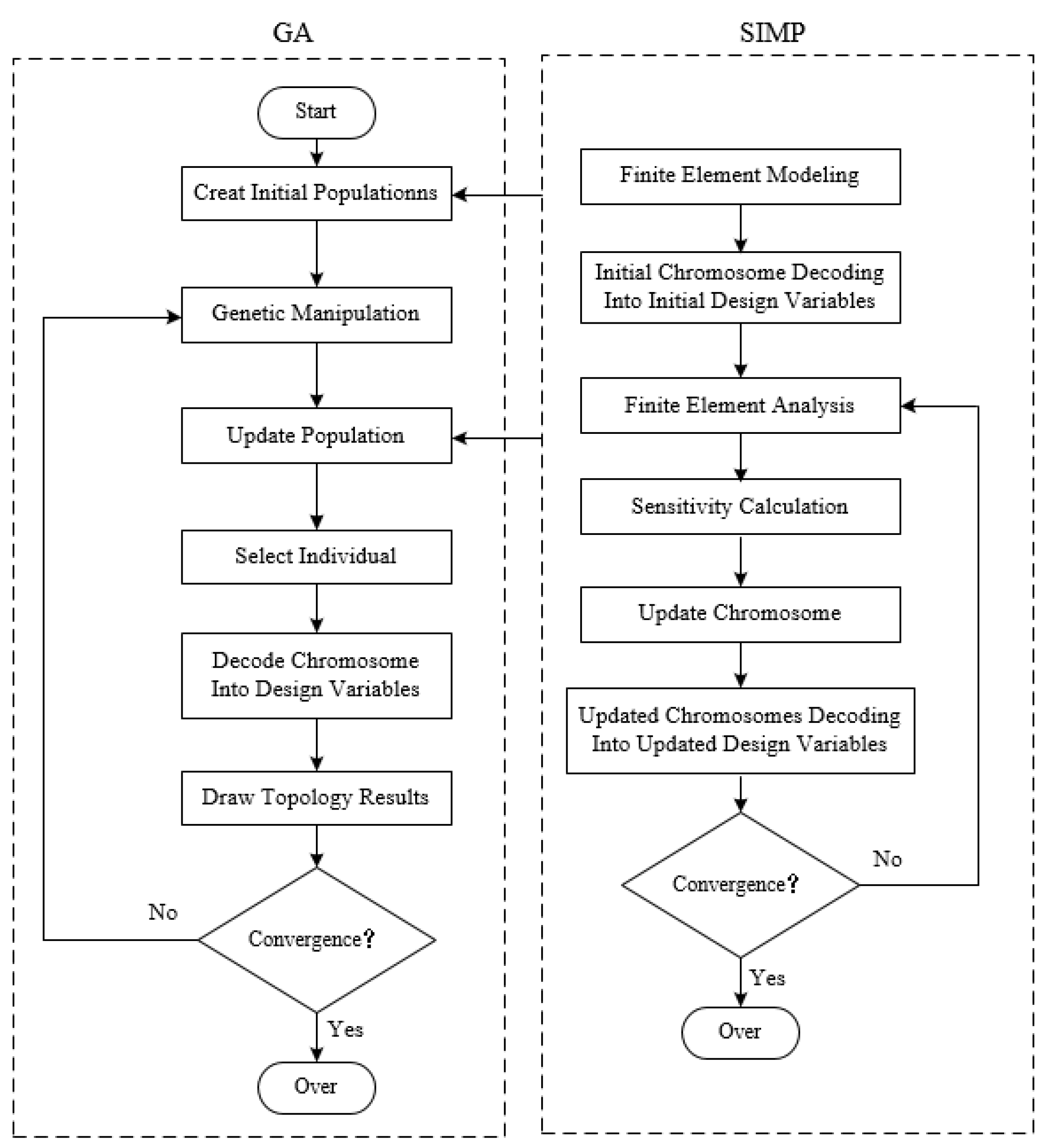
3. Implementation of the SIMP-GA Method

The genetic algorithm is a multi-point search method. Using multi-point search, the genetic algorithm can find different local optimal solutions, and during the search process new search points can be generated and more local optimal solutions can be sought. Simultaneously, in order to prevent all search points from falling into the local extreme value, the genetic algorithm has a mutation mechanism to ensure that the search can jump out of the local extreme value. These characteristics of the genetic algorithm ensure that it has a stronger global search capability.

A drawback of using the genetic algorithm is the huge amount of calculation it requires. Parallel genetic algorithm or micro-genetic algorithm is usually used to address this issue. In this paper, we propose a new topology optimization method to overcome the calculation costs required by the genetic algorithm. This method uses the sensitivity in the SIMP method to update the chromosomes in the genetic algorithm, which can accelerate convergence. In the SIMP-GA method, the genetic algorithm is used for optimization, while the population is updated during the process of optimization through gradient-based SIMP method design variable update criteria (Figure 1).

The genetic algorithm process is shown on the left of Figure 1. It uses general genetic algorithms and is easy to implement, for example, in MATLAB. First, the initial population is established, and then genetic operations are performed, that is, population crossover, mutation, and selection processes occur. Simultaneously, to obtain the topology results, a process of chromosome decoding into design variables and mapping topology results is added to display the optimization results. On the right of Figure 1 is the chromosomes update process based on the gradient SIMP method. The difference of this process from the conventional SIMP method is that instead of design variables, the chromosomes are updated in the process. It mainly performs finite element analysis, carries out objective function calculation and sensitivity calculation, decodes chromosomes into design variables, and updates chromosomes.

4. Examples and Calculation Process

4.1. MBB Beam

MBB beam is a common example used in structural topology optimization, so, for comparison, we also selected MBB beam as a case study analysis, as shown in Figure 2.

To reduce the number of calculations required, only half of the MBB beams are usually analyzed using symmetry. First, a 120 × 40 grid beam was selected for analysis. The volume fractions were set to 0.6, and the filter radii were set to 2, 3, and 4.

The optimization calculation process for MBB beams with grid elements was divided into 160 × 40, with filter radius and volume fractions of 2 and 0.5, respectively. It can be seen in Figure 3 that the SIMP-GA method generally produces good layout results after 10 iterations, and the results stabilized after 20 iterations, after which the topology layout basically does not change (Figure 3). Therefore, The SIMP-GA method converges after around 20 iterations (Figure 4). The algorithm used in the SIMP-GA method is shown in Appendix A.

An MBB beam with a grid density of 120 × 40 was then selected for analysis. We set the filter radius and volume fraction to 3 and 0.6, respectively. After running the SIMP-GA method 10 times, we obtained the results shown in Figure 5.

It can be seen from the optimization results that the randomness of the genetic algorithm means there is some variation in the results of each operation. Nevertheless, the average results obtained by the SIMP-GA method are better than those obtained by the SIMP method (

Table 1. Comparison of MBB beam optimization results.

Optimization Method	SIMP-GA			SIMP
	Best	Worst	Mean
$\mathrm{c}$	161.7409	163.6455	162.5064	173.2377

).

We then considered optimization results under different grid accuracy conditions. The above structures were divided into grids of 60 × 20, 150 × 50, and 300 × 100. The volume fraction was kept at 0.6 and the filter radius was set to 0.04 times the beam width, that is, for three beams, the filter radii were 2.4, 6, and 12, respectively. The optimization results obtained using the SIMP-GA method are shown in Figure 6.

The results obtained by the three grid division methods were basically the same, albeit with some slight local differences. This shows that by properly setting the filtering radius, the SIMP-GA method can obtain good optimization results and ensure structural connectivity.

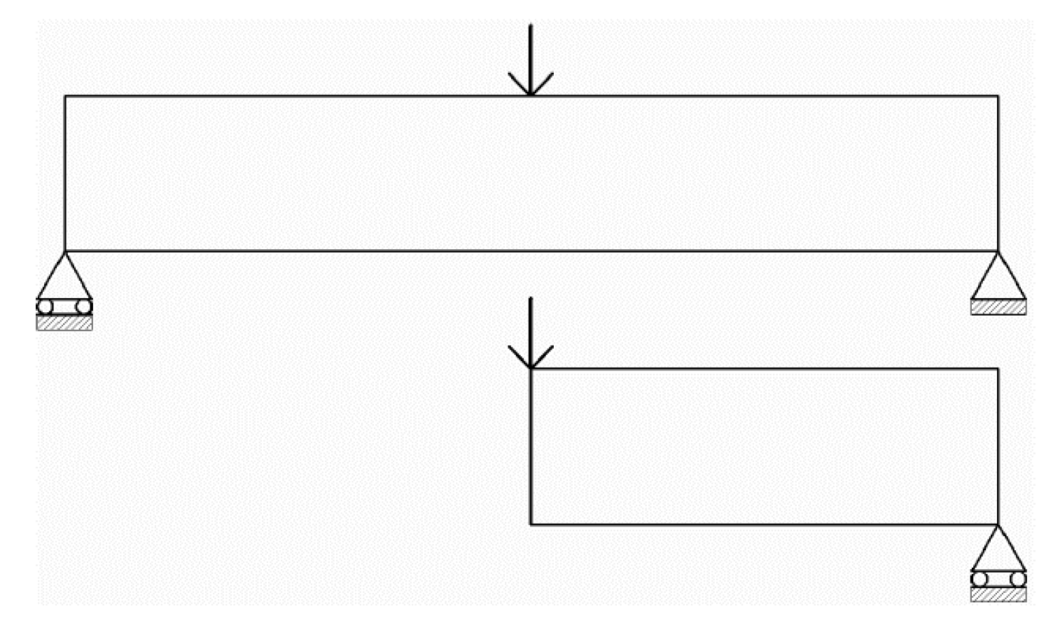
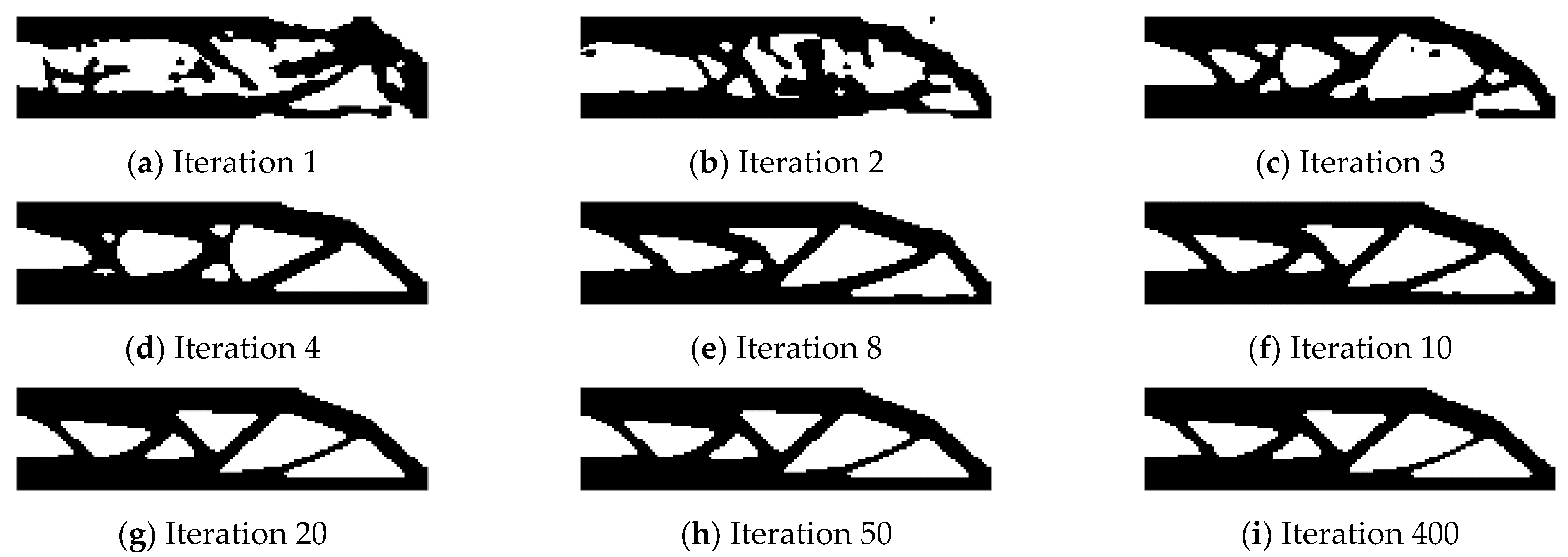
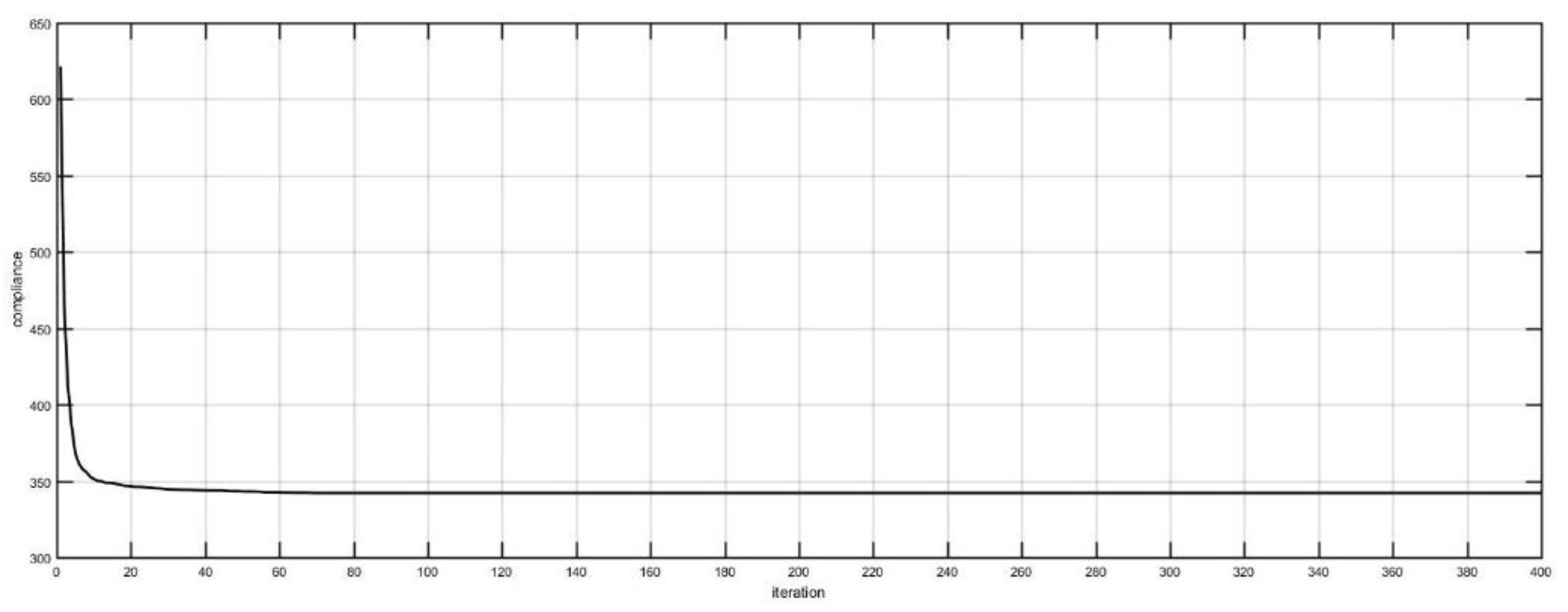
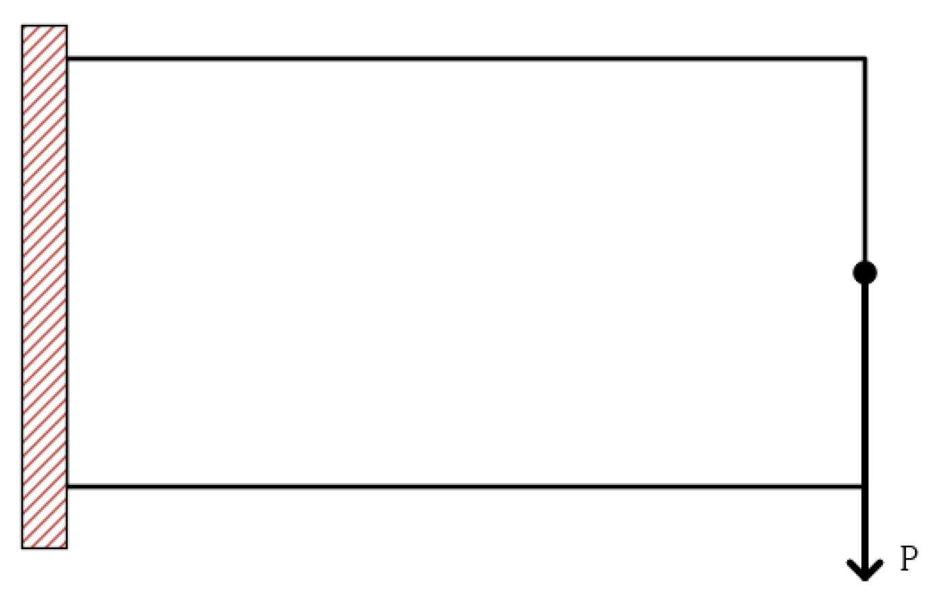
4.2. Cantilever Beam

The second example is a cantilever beam with an aspect ratio of 2:1, with the left end completely fixed and a vertical downward force acting on the right end at the midpoint. A simplified model of the cantilever beam is shown in Figure 7.

The results of 10 runs on the cantilever beam are shown in Figure 8. Of the 10 runs, the results from only two differed, while the layout for the other results was similar. However, compared with the SIMP method, the results obtained by the SIMP-GA method were better (

Table 2. Comparison of MBB beam optimization results.

Optimization Method	SIMP-GA			SIMP
	Best	Worst	Mean
$\mathrm{c}$	62.305	62.96	62.699	65.92

).

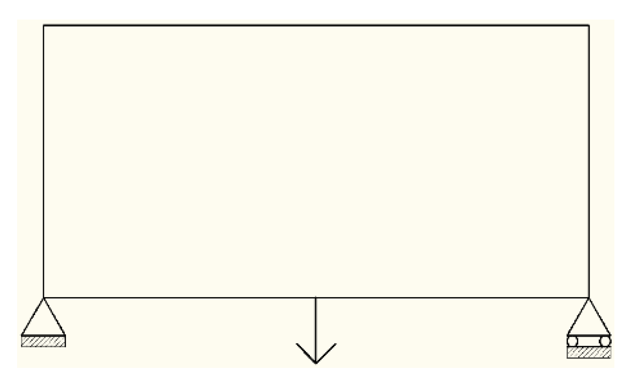
4.3. Half-Wheel Beam

A simplified model of a half-wheel beam is shown in Figure 9.

A cantilever beam with a grid density of 80 × 80 was then selected for analysis. We set the filtering radius and volume fraction to 3 and 0.6, respectively, and the SIMP-GA method was run 10 times. The results are shown in Figure 10.

5. Results and Comparison

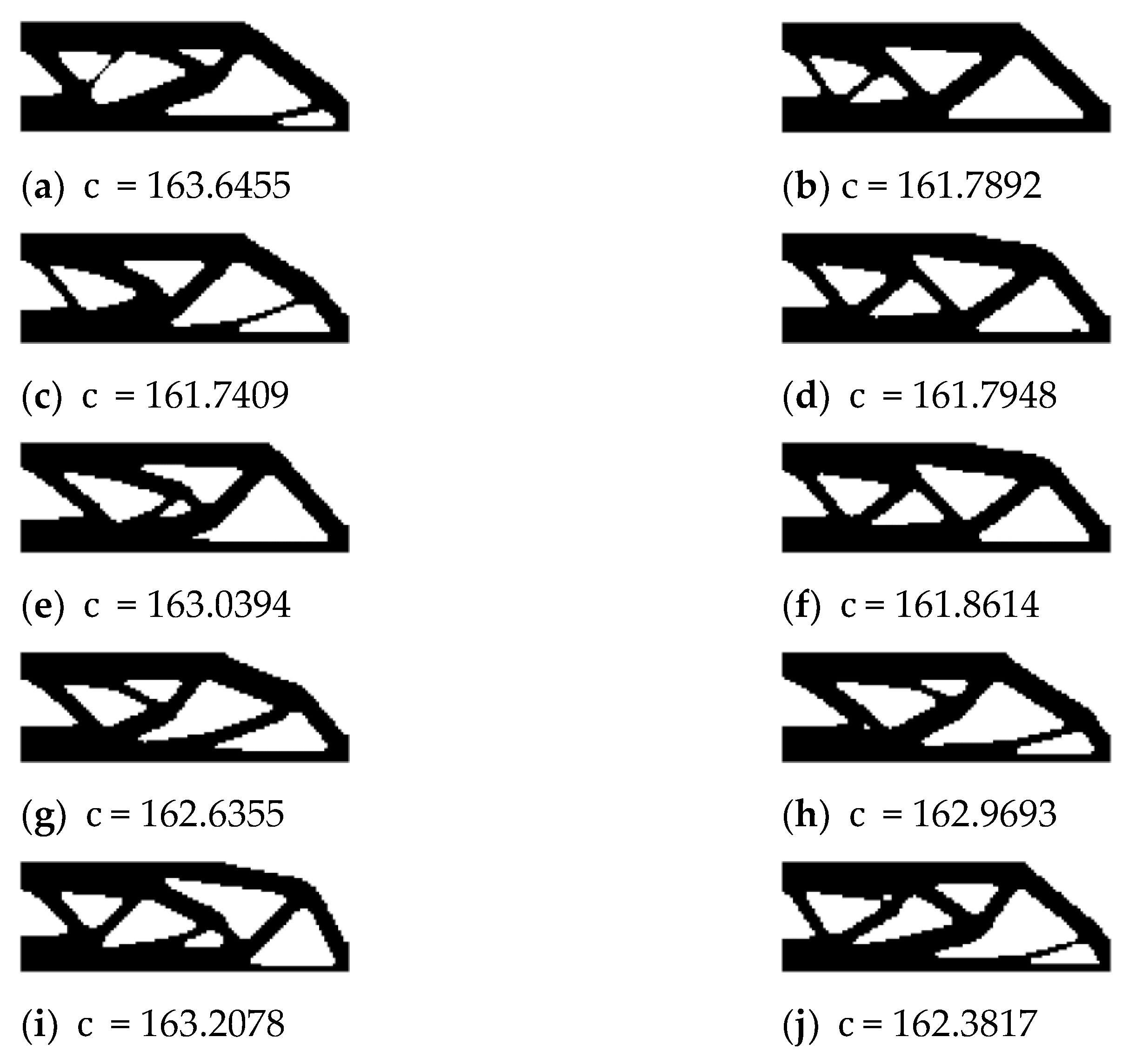
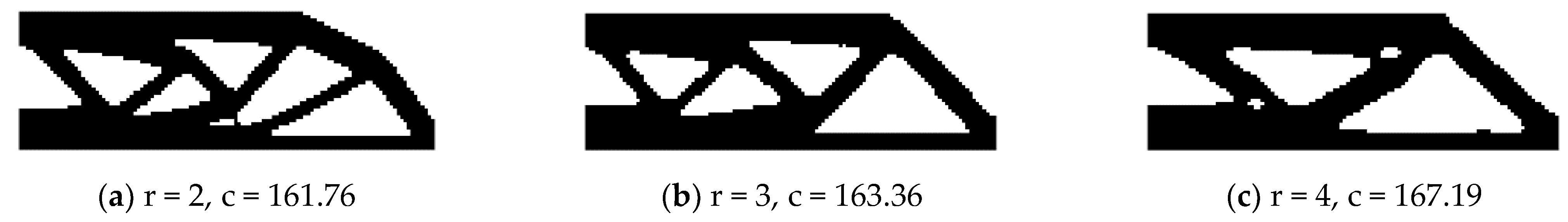
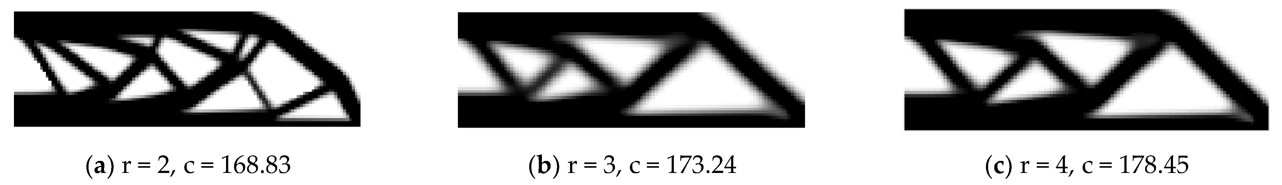
In this paper, the conventional genetic algorithm and SIMP method were combined. The conventional genetic algorithm and SIMP method program design are very mature, so this method is easy to implement and is conducive to commercialization. We utilized the code available in reference [29] and combined it with the MATLAB genetic algorithm toolbox to implement the program design documented in this paper.

5.1. MBB Beam

Using the SIMP-GA method, the structures shown in Figure 11 can be obtained.

In the SIMP method, the penalty factor is taken as 3, the volume fraction and the filtering radius are consistent with the above. The calculation results of the SIMP method are shown in Figure 12.

According to the optimization results, the objective function obtained by the SIMP-GA method is smaller and closer to the global optimal value. Simultaneously, because SIMP-GA does not directly update the design variables, the design variables are decoded by the chromosome into discrete 0 and 1 values, so there are no intermediate density elements in the optimized result, unlike if the SIMP method was used alone.

In the SIMP method, the geometric complexity of the optimization result can be controlled by a suitable filtering radius. The SIMP-GA method also inherits this characteristic. When the filtering radius is relatively small, the geometry obtained by SIMP-GA is more complex, but it is simpler than the SIMP method. When the filtering radius is appropriately increased, the results obtained by the SIMP-GA method are similar to those obtained by the SIMP method. As the filtering radius continues to increase, the geometric complexity of the optimization results obtained by the SIMP method remains effectively unchanged, but the structural geometry obtained by the SIMP-GA method is further simplified. Simultaneously, the intermediate density elements in the optimization results of the SIMP method also increase. If the filtering radius is too large, the intermediate density elements will fill the design area, making the optimization results unreliable. However, with the increase of the filtering radius, SIMP-GA can always obtain simpler geometric complexity results, as show in Figure 13.

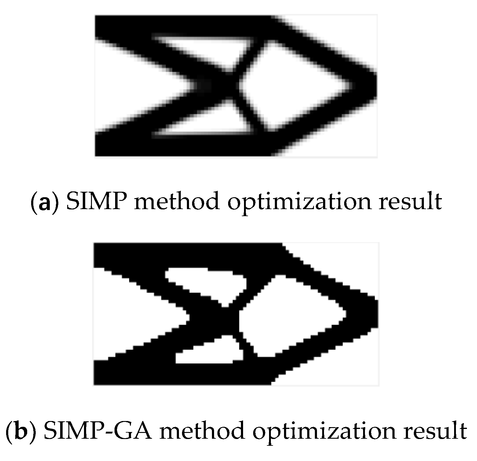
5.2. Cantilever Beam

The grid was divided into 80 × 40, giving a total of 3200 elements, the filtering radius was set to 2, and the volume fraction of the structure retention was 50%. The optimization results of the SIMP-GA method are shown in Figure 14b. The calculation results of the SIMP method are shown in Figure 14a.

Regarding the topological results, the results obtained by the five optimization methods [22,24,26] are similar. In the results obtained by conventional genetic algorithms, small-sized holes appeared [22,24]. The filtering methods were used in the SIMP-GA method, GA-BESO method, and SIMP method, which made the sensitivity function of the objective function smoother without mutation. Therefore, small-sized holes were suppressed, ensuring structural connectivity. Conventional genetic algorithms often require hundreds of generations of population to converge, and the calculation efficiency is low. It is not appropriate to use large-scale finite element meshes for calculations, so the topology results are not detailed enough. In the GA-BESO method, each element is an individual. When the finite element size is appropriate, the population size will not be too large and the calculation efficiency will be high. However, when the finite element mesh size is large the population size will increase and the calculation efficiency will be reduced. In the SIMP-GA method, a gene represents an element, and a certain number of populations can complete the calculation. Therefore, a large-scale grid can be used for calculation. At the same time, the SIMP-GA method uses the SIMP method to update the chromosomes, and compared with BESO, will update the population more efficiently. The GA-BESO method in reference [26] converged after 38 iterations, but in the SIMP-GA method, stable results were obtained after 20 iterations. Therefore, the calculation efficiency of the SIMP-GA method is higher than the conventional genetic algorithm and GA-BESO method.

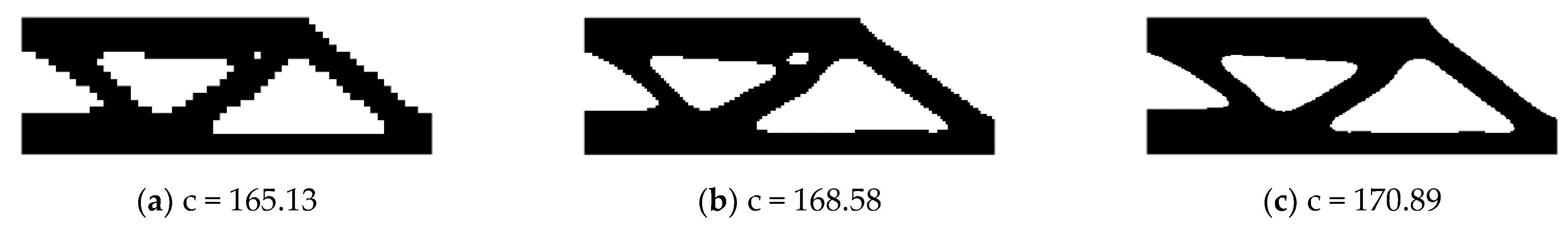
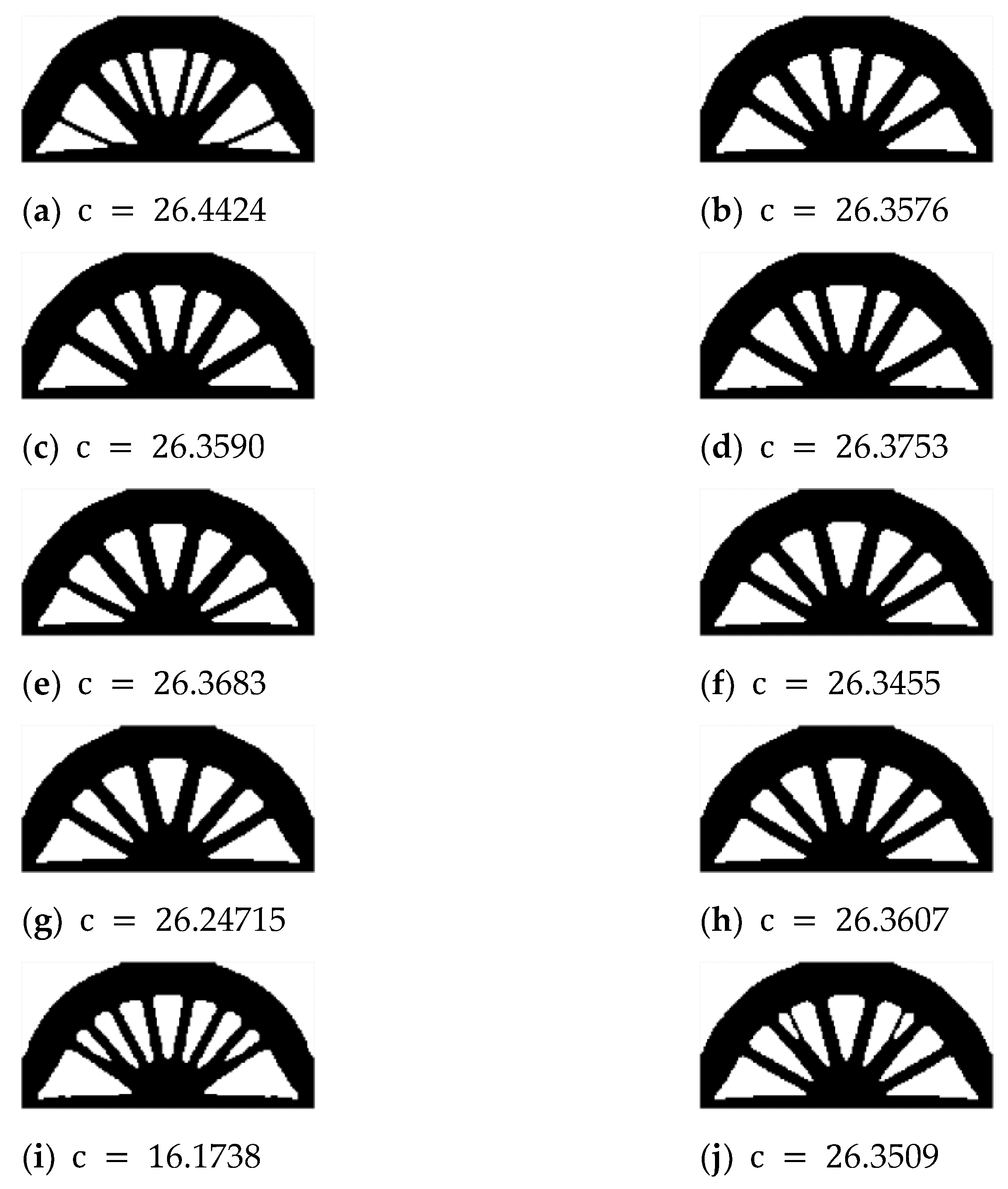
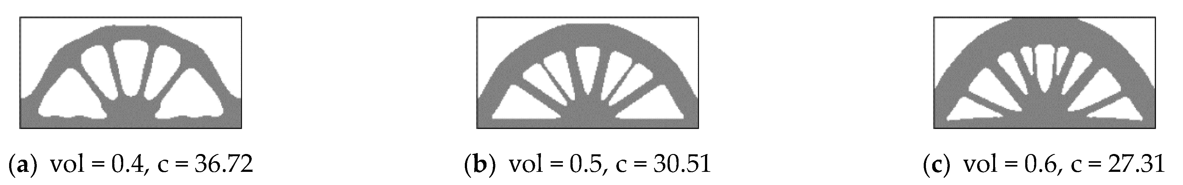
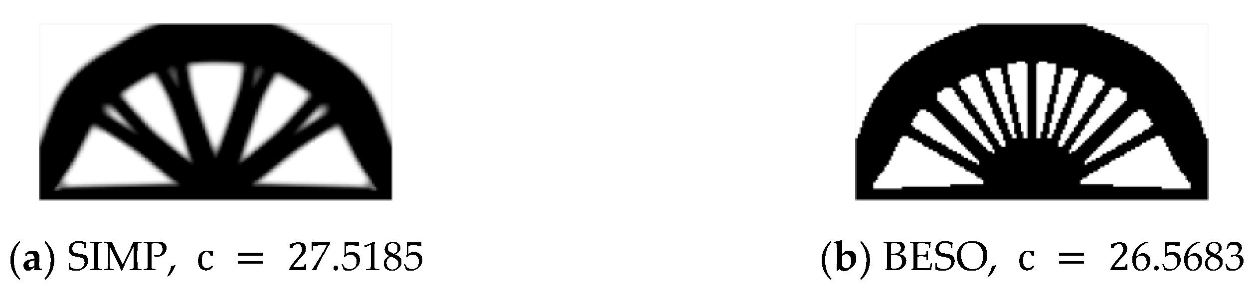
5.3. Half-Wheel Beam

For half-wheel beams, the optimization results under different volume fraction conditions using the SIMP-GA method are shown in Figure 15. The grid of the three half-wheel beams was divided into 100 × 100, the volume fractions were 0.4, 0.5, and 0.6, respectively, and the filter radius was 4.

The optimization results obtained using the SIMP and BESO methods are shown in Figure 16.

Using the SIMP-GA method over 10 runs, three results differed from the rest, which were all similar. In general, the objective function values obtained by the SIMP-GA method were smaller than those obtained by the SIMP and BESO methods (see in

Table 3. Comparison of half-wheel beam optimization results.

Optimization Method	SIMP-GA			SIMP	BESO
	Best	Worst	Mean
$\mathrm{c}$	26.1738	26.4424	26.3380	65.92	26.5683

). The geometric complexity of the results obtained by the three methods also slightly differed: The SIMP method had the lowest geometric complexity, while the BESO method had the highest, and the SIMP-GA method was intermediate.

5.4. Characteristics of Methods

Genetic algorithm has the ability of fast random search independent of the problem domain. It starts from the group, has potential parallelism, can compare multiple individuals at the same time, and has great robustness. The search uses evaluation function to inspire, its process is simple, and has scalability, so it is easy to combine with other algorithms. However, the programming implementation of genetic algorithm is more complex. First of all, we need to encode the problem, and then we need to decode the problem after finding the optimal solution. The search speed of the algorithm is relatively slow, and it takes more training time to get a more accurate solution. The algorithm has a certain dependence on the selection of the initial population, and can be improved by combining with some heuristic algorithms.

SIMP is essentially a simplified model of homogenization method. In the algorithm design, the direction of the material and the size of the hole are not considered, which reduces the number of design variables. The optimization algorithm has good convergence and simple sensitivity. The sensitivity calculation of discrete design based on finite element method can be carried out directly. It is suitable for combining more complex nonlinear structural topologies, such as geometric nonlinearity and material nonlinearity. However, the boundary of the topology optimized by simp method is not clear enough, especially when the filtering radius is large. These gray areas have no physical meaning, and the design cannot be directly used for manufacturing without post-processing.

The bi-directional evolutionary structural topology optimization method is proposed on the basis of the traditional evolutionary structural topology optimization method. This method is mainly used to solve topology optimization problems with certain material requirements. However, BESO method also has some problems, such as element deletion, chessboard form, mesh dependence, and so on.

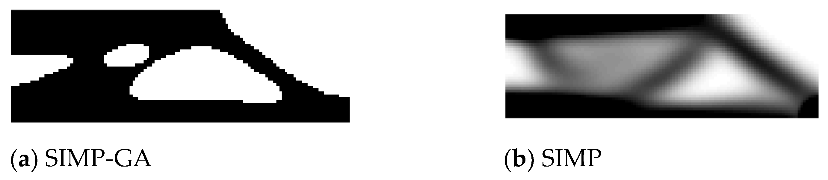
5.5. Comparison between Methods

From the previous examples, it can be seen that the SIMP-GA method does offer an advantage when searching for the global optimal solution. This is because the benefits of the SIMP method can be combined with those of the genetic algorithm. However, the genetic algorithm requires a large amount of calculation.

Under normal circumstances, compared with the SIMP method, the efficiency of the SIMP-GA method is relatively low. This is because SIMP-GA uses a multi-point search strategy, while the SIMP method is a single-point search method. Since the SIMP-GA method uses a multi-point search strategy, it can perform parallel calculations. When the parallel computing power is sufficient, the calculation efficiency of the SIMP-GA method can be improved.

5.6. Discussion

To compare the impact of parallel computing on the computational efficiency of the SIMP-GA method, we used a cantilever beam for analysis. The cantilever beam was divided into 120 $\times$ 75 grid elements, the population size was 50, and the number of iterations was 20. The CPU of the computer used was an i7-4790K, which has four working cores, and the single core clocked at 4 GHz. The calculation time consumed by the SIMP-GA method using different numbers of cores is shown in

Table 4. Influence of number of cores used on calculation efficiency when running the SIMP-GA method.

Number of cores	1	2	3
Calculating time (s)	173	95	72

.

The result showed that the calculation efficiency of the SIMP-GA method improved with the increasing number of working cores. In actual application, structural topology optimization method is often used in comparatively global structural design. As a kind of topology optimization method, SIMP-GA method will be used extensively in the lightweight structural design.

Although each different industry has its own structural specialty, they need a common topology optimized structure in production. They need a kind of topology optimized method to attain the goal. So the proposed SIMP-GA method can be as one of better choice. Such as in the geological exploration industry, the SIMP-GA method can be used to optimize the topology of the base of the drilling machine. In the automotive industry, the optimization principle of SIMP-GA method can be used to optimize the design of automotive engine components. In the aviation field, the SIMP-GA method can be used to optimize the flexible mechanism and trailing edge shape of the wing. As a structural topology optimization method, SIMP-GA method can be applied to more engineering fields in the future.

In the following research, based on the algorithm compilation of SIMA-GA, the efficiency of computation will improve significantly by introducing the genetic algorithm. In addition, simulated annealing algorithm and ant colony algorithm could also be introduced in the algorithm implementation of the SIMP-GA method and be sure to provide significant improvement in topology optimization.

6. Conclusions

In this paper, we proposed a novel topology optimization method to help lightweight design. We combined the SIMP method and genetic algorithm, and proposed a new topology optimization method, called SIMP-GA. By combining the two methods, SIMP-GA overcomes the shortcomings of the weak global search capability of SIMP and the large calculation requirements of the genetic algorithm. The material distribution of the optimized results obtained by the SIMP-GA method conforms to a 0–1 discrete distribution, which avoids the appearance of intermediate density elements that occur when using the SIMP method alone. The objective function value obtained by the SIMP-GA method is also lower than the values obtained by the SIMP and BESO methods. This shows that the optimization results obtained by SIMP-GA were better than those of the SIMP and BESO methods. Compared with the conventional genetic algorithm and GA-BESO method, the SIMP-GA method obtained similar topological results, but the SIMP-GA method has relatively high computing efficiency. The population size of the genetic algorithm in SIMP-GA is certain and will not increase with an increase in the number of grids, so large-scale grid computing can be adopted.

Obviously, with this method, it is easy to obtain a lighter weight structure. If this method is applied to various engineering fields, it can effectively realize the lightweight design of the structure and improve the performance of the structure.

References

1. Bendsøe, M.P.; Kikuchi, N. Generating optimal topologies in structural design using a homogenization method. Comput. Methods Appl. Mech. Eng. 1988, 71, 197–224. [Google Scholar] [CrossRef]
2. Bendsøe, M.P. Optimal shape design as a material distribution problem. Struct. Multidiscip. Optim. 1989, 1, 193–202. [Google Scholar] [CrossRef]
3. Mlejnek, H.P. Some aspects of the genesis of structures. Struct. Multidiscip. Optim. 1992, 5, 64–69. [Google Scholar] [CrossRef]
4. Stolpe, M.; Svanberg, K. An alternative interpolation scheme for minimum compliance optimization. Struct. Multidiscip. Optim. 2001, 22, 116–124. [Google Scholar] [CrossRef]
5. Xie, Y.M.; Steven, G.P. Basic Evolutionary Structural Optimization; Springer: Berlin/Heidelberg, Germany, 1997. [Google Scholar]
6. Young, V.; Querin, O.M.; Steven, G.P. 3D and multiple load case bi-directional evolutionary structural optimization (BESO). Struct. Optim. 1999, 18, 183–192. [Google Scholar] [CrossRef]
7. Querin, O.M.; Steven, G.P.; Xie, Y.M. Evolutionary structural optimisation (ESO) using a bidirectional algorithm. Eng. Comput. 1998, 15, 1031–1048. [Google Scholar] [CrossRef]
8. Querin, O.M.; Young, V.; Steven, G.P. Computational efficiency and validation of bi-directional evolutionary structural optimization. Comput. Methods Appl. Mech. Eng. 2000, 189, 559–573. [Google Scholar] [CrossRef]
9. Xia, Q.; Shi, T.L. Generalized hole nucleation through BESO for the level set based topology optimization of multi-material structures. Comput. Methods Appl. Mech. Eng. 2019, 355, 216–233. [Google Scholar] [CrossRef]
10. Sethian, J.A. Level Set Methods and Fast Marching Methods: Evolving Interfaces in Computational Geometry, Fluid Mechanics, Computer Vision, and Materials Science; Cambridge University Press: Cambridge, UK, 1999. [Google Scholar]
11. Wang, Y.; Kang, Z. Structural shape and topology optimization of cast parts using level set method. Int. J. Numer. Methods Eng. 2017, 111, 1252–1273. [Google Scholar] [CrossRef]
12. Holland, J.H. Adaptation in Natural and Artificial Systems; The University of Michigan Press: Ann Arbor, MI, USA, 1975. [Google Scholar]
13. Vaissier, B.; Pernot, J.P.; Chougrani, L.; Véron, P. Genetic-algorithm based framework for lattice support structure optimization in additive manufacturing. Comput. Aided Des. 2019, 110, 11–23. [Google Scholar] [CrossRef]
14. Goldberg, D.E.; Samtani, M.P. Engineering optimization via genetic algorithms. In Electronic Computation, Proceedings of the 9th Conference on Electronic Computation, Birmingham, UK, 23–26 February 1986; Amer Society of Civil Engineers: Reston, VA, USA, 1986. [Google Scholar]
15. Sigmund, O. A 99 line topology optimization code written in Matlab. Struct. Multidiscip. Optim. 2001, 21, 120–127. [Google Scholar] [CrossRef]
16. Zhu, B.; Skouras, M.; Chen, D.; Matusik, W. Two-scale topology optimization with microstructures. Acm Trans. Graph. 2017, 84, 1–19. [Google Scholar] [CrossRef] [Green Version]
17. Otomori, M.; Yamda, T.; Izui, K. Matlab code for a level set-based topology optimization method using a reaction diffusion equation. Struct. Multidiscip. Optim. 2015, 51, 1159–1172. [Google Scholar] [CrossRef] [Green Version]
18. Huang, X.; Xie, Y.M. Evolutionary topology optimization of continuum structures including design-dependent self-weight loads. Finite Elem. Anal. Des. 2011, 47, 942–948. [Google Scholar] [CrossRef]
19. Rozvany, G. A critical review of established methods of structural topology optimization. Struct. Multidiscip. Optim. 2009, 37, 217–237. [Google Scholar] [CrossRef]
20. Hajela, P.; Lee, E. Genetic algorithms in truss topological optimization. Int. J. Solids Struct. 1995, 32, 3341–3357. [Google Scholar] [CrossRef]
21. Wang, S.Y.; Tai, K. Structural topology design optimization using Genetic Algorithms with a bit-array representation. Comput. Methods Appl. Mech. Eng. 2005, 194, 3749–3770. [Google Scholar] [CrossRef]
22. Wang, S.Y.; Tai, K.; Wang, M.Y. An enhanced genetic algorithm for structural topology optimization. Int. J. Numer. Methods Eng. 2006, 65, 18–44. [Google Scholar] [CrossRef]
23. Jakiela, M.J.; Chapman, C.; Duda, J. Continuum structural topology design with genetic algorithms. Comput. Methods Appl. Mech. Eng. 2000, 186, 339–356. [Google Scholar] [CrossRef]
24. Fanjoy, D.W.; Crossley, W.A. Topology Design of planar cross-sections with a genetic algorithm: Part 1—Overcoming the obstacles. Eng. Optim. 2002, 34, 1–22. [Google Scholar] [CrossRef]
25. Liu, X.; Yi, W.J.; Li, Q.S. Genetic evolutionary structural optimization. Steel Constr. 2004, 64, 305–311. [Google Scholar] [CrossRef]
26. Zuo, Z.H.; Xie, Y.M.; Huang, X. Combining genetic algorithms with BESO for topology optimization. Struct. Multidiscip. Optim. 2009, 38, 511–523. [Google Scholar] [CrossRef]
27. Chen, Z.M.; Gao, L.; Qiu, H.B.; Shao, X.Y. Combining genetic algorithms with optimality criteria method for topology optimization. In Proceedings of the 2009 Fourth International on Conference on Bio-Inspired Computing, Beijing, China, 16–19 October 2009. [Google Scholar]
28. Qu, D.Y.; Huang, Y.Y.; Song, L.Y. Structural topology optimization based on improved genetic algorithm. In Proceedings of the 4nd International Conference on Mechanical Engineering and Green Manufacturing (MEGM2015), Guilin, China, 30–31 August 2015. [Google Scholar]
29. Andreassen, E.; Clausen, A.; Schevenels, M. Efficient topology optimization in MATLAB using 88 lines of code. Struct. Multidiscip. Optim. 2011, 43, 1–16. [Google Scholar] [CrossRef] [Green Version]
Figure 1. SIMP-GA algorithm flow.
Energies 14 04367 g001
Figure 2. The MBB beam.
Energies 14 04367 g002
Figure 3. Optimization results at different stages.
Energies 14 04367 g003
Figure 4. Variation of objective function with iteration steps.
Energies 14 04367 g004
Figure 5. Final results from 10 runs of the MBB beam.
Energies 14 04367 g005
Figure 6. Optimization results with different mesh sizes.
Energies 14 04367 g006
Figure 7. Cantilever beam model.
Energies 14 04367 g007
Figure 8. Final results from 10 runs of cantilever beam.
Energies 14 04367 g008
Figure 9. Simplified model of half-wheel beam.
Energies 14 04367 g009
Figure 10. Final results from 10 runs of half-wheel beam.
Energies 14 04367 g010
Figure 11. Optimization results of the SIMP-GA method.
Energies 14 04367 g011
Figure 12. Optimization results of the SIMP method.
Energies 14 04367 g012
Figure 13. Optimization result when r = 8.
Energies 14 04367 g013
Figure 14. Comparison of results obtained using different optimization methods: (a) SIMP method optimization result; (b) SIMP-GA method optimization result.
Energies 14 04367 g014
Figure 15. Optimization results of half-wheel beams with different volume fractions.
Energies 14 04367 g015
Figure 16. Optimization results of SIMP and BESO methods.
Energies 14 04367 g016