Energy and Exergy (2E) Analysis of an Optimized Solar Field of Linear Fresnel Reflectors for a Conceptual Direct Steam Generation Power Plant

Abstract

Direct steam generation is a promising alternative to conventional heat transfer fluids for solar thermal power plants using linear concentrators because water and steam do not have thermal and chemical stability problems. The novelty of this study, an energy and exergy (2E) analysis, was that it was performed on several configurations of a conceptual direct steam generation solar power plant with optimized Fresnel reflectors in Agua Prieta, Mexico coupled with a regenerative steam Rankine power cycle to quantify their efficiency and establish a reference for future implementation of this technology in concentrated solar power plants in Mexico. The thermal model was assumed to be a 1D steady-state flow and validated against results in the literature. It was then applied directly to a case study to determine the size of the solar field. The design point was the lowest solar irradiance day, and evaluating the solar multiple with the highest solar irradiance, taking care not to oversize the solar field, as suggested for solar plants without energy storage. Comparing the performance of the optimized Fresnel field against the FRESDEMO field of Plataforma Solar de Almería, a considerable decrease in the length of the loop has been demonstrated with a low reduction in thermal efficiency.

1. Introduction

In recent years, the towering environmental problems faced around the world have increased the urgency to incorporate technologies for harvesting renewable resources to satisfy energy demand. In 2018, the global energy demand was estimated to be 556 E, of which 88.3 EJ was for generating electricity [1]. As an alternative to fossil fuels, solar technologies such as concentrated solar power (CSP) have been added to the energy mix. CSP uses different mirror configurations to concentrate the incident solar radiation onto a smaller area called a receiver, where high heat is supplied to a heat transfer fluid (HTF) that is used to drive a heat engine and generate electric power.

Any attempts to optimize a process to increase its efficiency will directly influence the system’s energy inputs and outputs. The authors’ present work is focused on optimizing the configuration of the FRESDEMO field (demonstration module of a Linear Fresnel Collector) developed in the Plataforma Solar de Almeria (PSA), which is the reference field that uses linear Fresnel reflectors (LFRs) for direct steam generation (DSG) [2]. The considered optimization maintains similar parameters to the FRESDEMO field, which allows the amount of energy on the receiver to be increased [3].

DSG was introduced in the 1990s as an alternative to parabolic through collectors (PTC) driven steam Rankine cycles using an HTF, to reduce the system’s capital and maintenance costs [4,5], and several studies were performed to sort the problems associated with bending [6,7]. However, the absence of a storage system or an intermediate HTF results in adapting the intermittent nature of the solar energy limiting the controllability and stability of the whole installation, as demonstrated in the early 2000s [8,9].

Even though DSG has begun to gain popularity because of the reduced costs of the associated equipment, currently there are few commercial plants using DSG technology, in contrast to one of the objectives laid out by the International Energy Agency (IEA), which predicted that the introduction of DSG at the commercial level would occur by the late 2010s [10]. To date, there are about 110 operational plants [11], with an installed capacity of 6289 MW [12]. Of the total installed, just over 522 MW are obtained through DSG, of which the power towers make the greatest contribution with 90.9%, LFRs contribute 7.7%, and only the 5 MW Thai Solar Energy 1 plant uses PTC [11]. A brief review of the coupling of DSG and CSP is shown in

Table 1. Solar thermal plants operating with DSG Rankine cycle [11].

Name	Technology	Capacity (MW)	Storage/Back Up	Status
Greenway CSP Mersin (Turkey)	Power tower	1	Molten salt tank	Non-operational
Puerto Errado 1 (Spain)	LFR	1.4	Single thermocline tank	Operational
Sundrop (Australia)	Power tower	1.5	No storage	Operational
Lake Cargelligo (Australia)	Power tower	3	Graphite thermal storage	Non-operational
Liddell Power Station (Australia)	LFR	3	No storage	Non-operational
Thai solar one (Thailand)	PTC	5	No storage	Operational
Kimberlina (USA)	LFR	5	No storage	Non-operational
Sierra SunTower (USA)	Power tower	5	No storage	Non-operational
eLLO (France)	LFR	9	Steam drum	Operational
PS10 (Spain)	Power tower	11	Heat storage	Operational
Dadri ISCC Plant (India)	LFR	14	Not specified	Under construction
PS20 (Spain)	Power tower	20	Heat storage	Operational
Puerto Errado (Spain)	LFR	30	Single thermocline tank	Operational
Khi Solar One (Spain)	Power Tower	50	Steam drum	Operational
Shangyi Tower (China)	Power Tower	50	2 molten salt tanks	Under development
Zhangbei (China)	LFR	50	Solid-state formulated concrete	Non-operational
Zhangjiakou (China)	LFR	50	Solid-state formulated concrete	Under development
Huanghe Qinghai Delingha (China)	Power Tower	135	2 molten salt tanks	Non-operational
Ivanpah (USA)	Power Tower	392	No storage	Operational

.

While both DSG and LFRs have high implementation potential, their development has not yet reached the necessary maturity to make them commercially viable as PTCs using thermal oils as HTF. For this reason, an energy and exergy analysis (2E) of an optimized Fresnel field with DSG coupled to different configurations of Rankine cycles is needed to establish a reference for its future implementation in Mexico. The 2E analysis is necessary for objectively comparing any systems. Although the energy analysis is suitable for determining the efficiency of a system, it does not give information on the quality and locations of imperfections in the system. Exergy analysis serves as a tool for identifying the magnitude and location of irreversibilities in thermal systems [13,14,15,16].

One of the most representative thermal analyses on CSP with DSG was by Montes Pita [4], who considered different solar field configurations for varying operating conditions and materials. This work gives a starting point for the thermal analysis of LFRs for DSG. Giostri et al. [17] compared the thermal performance of two solar plants using thermal oil as the HTF with PTCs and with LFRs. Although they also simulated DSG with LFRs, this was not compared with the others. They proved that a solar field using DSG performs better than one using oil under the same operating conditions. Hirsch and Khenissi [18] demonstrated that superheating is a viable alternative at moderate temperatures (≤450 °C) and pressures lower than 14 bar in solar plants with 50 MW DSG. Although they did not explain what type of concentrator they used (PTC or LFR), the large number of parameters that were considered in their simulations indicates that their work can be used as a reference for operating conditions.

Sun et al. [19] numerically simulated a solar plant with PTCs in recirculation and performed a 2E analysis. However, their model does not specify the power output of the solar plant. Hakkarainen et al. [20] compared two configurations for DSG using PTCs and LFRs. They showed that the LFR field needs to be almost twice the size of the PTC field to achieve the same thermal power output for the solar plant, although they did note that LFRs provide better controllability than PTCs over DSG.

Although different groups have performed thermal analyses on LFR solar fields, the vast majority performed a 2E analysis on a single configuration or single power range, which limited the comparison of results to demonstrating the technical feasibility of using LFRs with DSG. Thus, the objective of the present study intends to describe a conceptual direct steam generation solar power plant for Agua Prieta, Mexico with different configurations for the solar field and a Rankine cycle, and compare the results with the FRESDEMO field.

A starting point was established by determining the configurations of 10 MW regenerative Rankine cycles and quantifying the required thermal power output of the optimized solar field. A thermo-hydraulic model was developed to consider different aspects of establishing the heat fluxes and surface temperatures of the elements involved in the receiver based on the methodology proposed by Adiutori [21], where the use of the heat transfer coefficient is omitted to avoid the iterative process involved in its determination. This allowed a direct solution to be obtained for all variables involved. The developed model is versatile and can be used to study the behavior of the system with different working fluids simply by changing the thermodynamic properties of the working fluid. Finally, configurations of the solar field were established to set the field dimensions for meeting the operating requirements of the proposed Rankine cycles. The solar multiple was determined for the conditions with the highest and lowest insolation.

2. Characterization of Thermodynamic Cycles

Even though the objective of this work was a 2E analysis of the LFR system, characterizing the thermodynamic cycle will allow the theoretical efficiency of the Rankine cycle configurations to be determined. Maximizing the work output (i.e., improving the thermal efficiency) depends on the available energy supplied as heat in the steam generator, the output of the system (turbine work), and the work required to operate the pumps that are part of the cycle. While increasing the work output, the entropy generation in the cycle is minimized as stated by the Guoy-Stodola theorem [22]. Thus, when considering the net power output of the system, the amount of heat needed in the steam generator can be quantified to define the size of the solar field, as described in Section 3. A Rankine cycle can have a reheating or regeneration configuration. For solar-only power plants, regeneration is preferred [23]. Under this premise, a regenerative steam Rankine cycle was the configuration used in the present study. The goal of the thermodynamic characterization was to establish the thermodynamic state of each flow of mass, energy, entropy, and exergy involved in the cycle to quantify the useful power output of the system and identify the irreversibilities in the power cycle [24,25].

2.1. Operating Parameters of the Regenerative Rankine Cycle

An important consideration for the analysis of power systems is determining the design points (i.e., boundary conditions), which are the settings under which the power block will be operating under nominal conditions. The following design points were identified for a power plant similar to the FRESDEMO project [15]: net power output of 10 MW, pressure of 100 bar, and temperature of 400 °C (673.15 K) of steam at the turbine inlet, and pressure of 0.08 bar at the turbine outlet. The turbine, which is the most important component of a thermoelectric plant, must be selected according to these design points. Considering the steam conditions and net power output of the system, a Siemens SST-200 turbine with a nominal isentropic efficiency of 80% [26] was selected because it can adequately handle the proposed power ranges and its characteristics are adapted to the standards of the simulations [27].

The number and location of extraction points for preheating the feed water in a given plant is a significant consideration. Although using many regenerators results in higher exergy efficiency, this leads to overly complicated operations and has a substantial impact on the installation costs [28]. The extraction of steam in the turbine reduces the nominal isentropic efficiency [29]. In the present work, two configurations were considered for the steam Rankine cycles: two and three steam extractions. Since the only given data were the pressures at the inlet and outlet of the turbine, the location of the extraction points in the system (extraction pressures) was optimized to maximize the efficiency of the power cycle, according to the criterion established in the literature to minimize the exergy destruction [28,30]. This made it possible to quantify the thermal energy necessary for the operation of the power cycles.

2.2. Analyzed Cycles

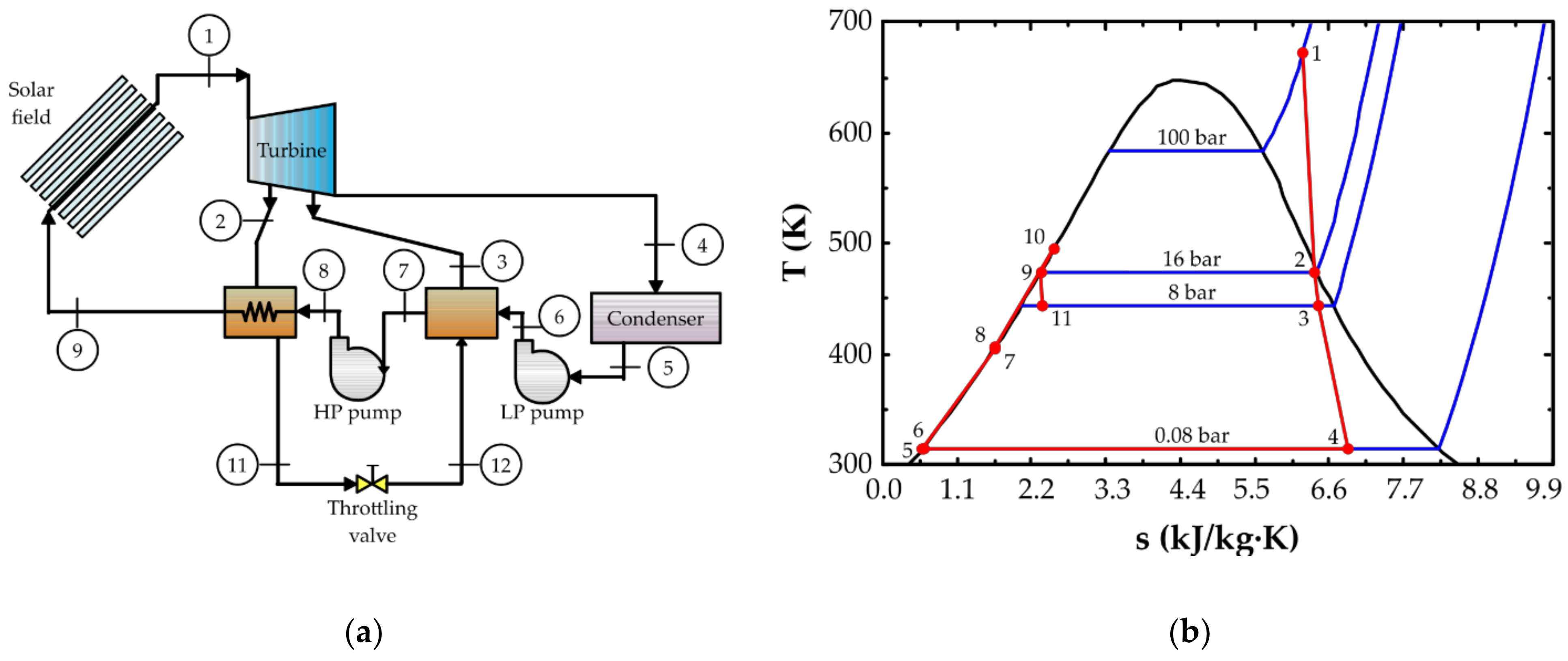
2.2.1. Regenerative Cycle with two Steam Extractions

Figure 1a shows a schematic of the configuration of the steam Rankine cycle. To define each thermodynamic state, the steam extraction pressure was determined in a sensitivity analysis. This sensitivity analysis was performed comparing the variation of the exergy efficiency in the power block (excluding the solar field) for different values of the extraction pressure. As a result, power block exergy efficiency was maximized around 8 bar. This pressure was used to characterize the cycle, as presented in

Table 2. Two steam extractions regenerative Rankine cycle thermodynamic characterization.

State	Ti(K)	Pi(bar)	hi(kJ/kg)	si(kJ/kg K)	bi(kJ/kg)	xi
1	673.2	100	3097.4580	6.2141	1249.2832	superheatedsteam
2	474.5	16	2775.6092	6.3837	876.8784	0.9911
3	443.6	8	2672.1738	6.4449	755.1900	0.9530
4	314.7	0.08	2153.1660	6.8829	105.5952	0.8239
5	314.7	0.08	173.8396	0.5925	1.7490	0
6	314.7	8	174.9044	0.5933	2.5616	liquid
7	404.6	8	552.4712	1.6497	65.1769	0
8	406.3	100	566.3182	1.6582	76.4810	liquid
9	496.1	100	959.3855	2.5312	209.2742	liquid
10	474.5	16	858.4440	2.3435	164.3041	0
11	443.6	8	858.4440	2.3858	160.6143	0.0672

and the T–s diagram of Figure 1b. A mass flux of 12.81 kg/s is required to achieve a net power output of 10 MW. The obtained results indicated an energy efficiency of 0.3652 (i.e., 36.52%) and exergy efficiency of 0.8247 (i.e., 82.47%).

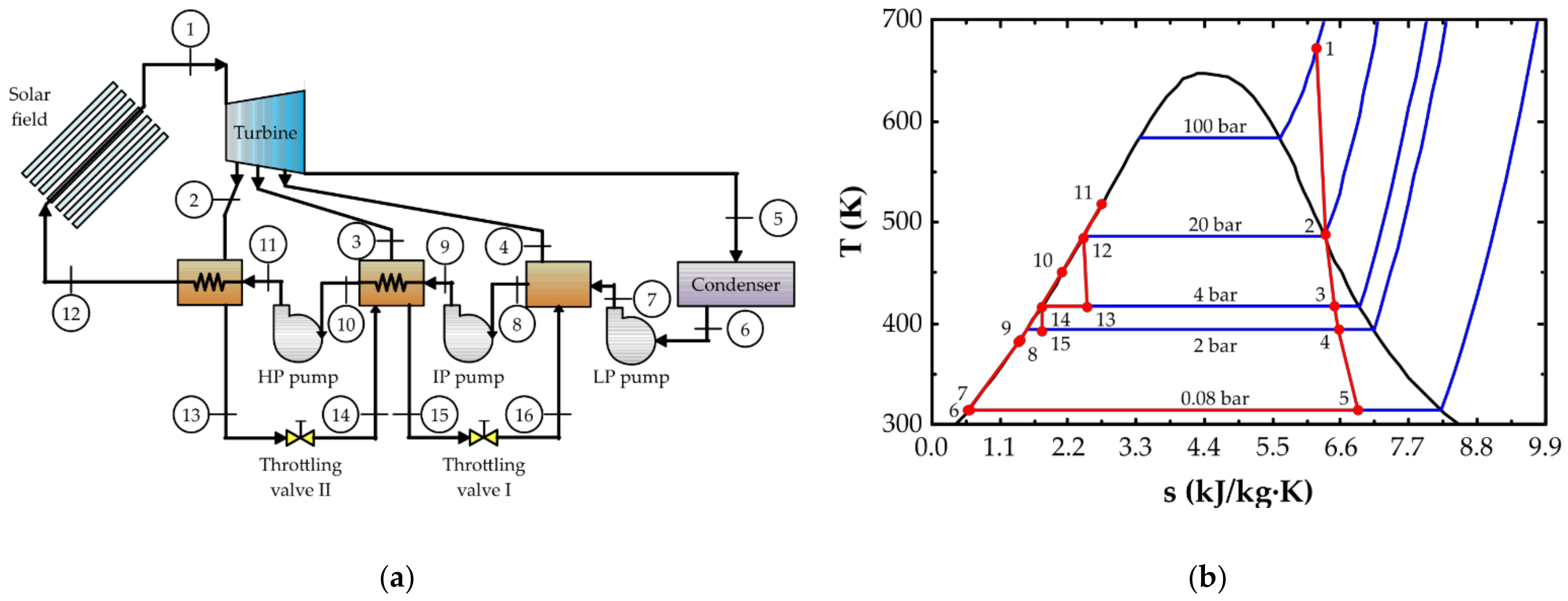
2.2.2. Regenerative Cycle with Three Steam Extractions

Figure 2a shows a schematic of the second configuration of the power cycle. Like the previous case, a sensitivity analysis was carried out to establish the extraction pressures that maximize the exergy efficiency of the power block. This maximization resulted in a pressure of 20 bar for the first extraction, 4 bar for the second extraction, and 2 bar for the last extraction. The thermodynamic states of the ith-flows are reported in

Table 3. Three steam extraction regenerative Rankine cycle thermodynamic characterization.

State	Ti(K)	Pi(bar)	hi(kJ/kg)	si(kJ/kg K)	bi(kJ/kg)	xi
1	673.2	100	3097.4580	6.2141	1249.2832	superheated steam
2	489.1	20	2809.6092	6.3622	917.2702	superheated steam
3	416.8	4	2576.3714	6.5075	640.7096	0.9242
4	393.4	2	2486.6878	6.5688	532.7680	0.9003
5	314.7	0.08	2147.8559	6.8660	105.3166	0.8217
6	314.7	0.08	173.8396	0.5925	1.7490	0
7	314.7	2	174.0977	0.5927	1.9460	liquid
8	382.1	2	456.7724	1.4067	41.9233	0
9	383.6	100	470.5577	1.4157	53.0272	liquid
10	451	100	758.2368	2.1063	134.8163	liquid
11	518.4	100	1062.9448	2.7353	251.9609	liquid
12	485.5	20	908.4743	2.4467	183.5490	0
13	416.8	4	908.4743	2.5055	166.0308	0.1424
14	416.8	4	604.6573	1.7765	79.5653	0
15	393.4	2	604.6573	1.7843	77.2359	0.0454

and the T–s diagram of Figure 2b. The results indicated an energy efficiency of 0.3706 (i.e., 37.06%) and an exergy efficiency of 0.8661 (i.e., 86.61%). A net power output of 10 MW requires 13.26 kg/s of water.

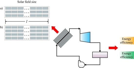
3. Solar Field: Linear Fresnel Reflector

Although the optical description of LFRs is simple, many parameters need to be considered for the design of LFR systems. However, very little data are available to describe an LFR field [31]. Based on the descriptions for different LFR designs, the FRESDEMO field located at Plataforma Solar de Almería in Spain was selected as a starting point.

The parameters of the FRESDEMO field were taken as a reference to perform an optical optimization for the city of Agua Prieta, Sonora, in northwest México. The optimization of the intercept factor resulted in an increase in the receiver height from 8 m to 15 m, and the compound parabolic concentrator (CPC) of the second stage of the cavity was modified to maintain the opening area of the receiver [3]. As a result of the performed optimization, the average optical concentration increases from 61.64 to 79.31. This increase will lead to a significant reduction in the loop length of the solar field.

Table 4. Description of the optically optimized LFR field for Agua Prieta, Sonora [3].

Parameter	Value
Number of primary mirrors	25
Solar field width (m)	21
Total length of the primary mirrors (m)	100
Width of the primary mirrors (m)	0.6
Filling factor	0.7143
Receiver height (m)	15
Receiver width (m)	0.5
Absorber tube outer diameter (m)	0.14
Absorber tube inner diameter (m)	0.125
Semi-angle acceptance of the CPC (°)	66.30
Intercept factor	0.7231
Geometric concentration of the CPC	1.1368
Geometric concentration of the entire field	34.105
Number of supports per module	17

describes the parameters of the optimized field. Figure 3 shows the incident angle modifiers (IAMs) that were determined for the optimized LFR; these represent the changes in optical efficiency for angles of incidence other than perpendicular. Figure 4 shows the relation between the variation in the average optical concentrator on the plane of the absorber and the IAMs.

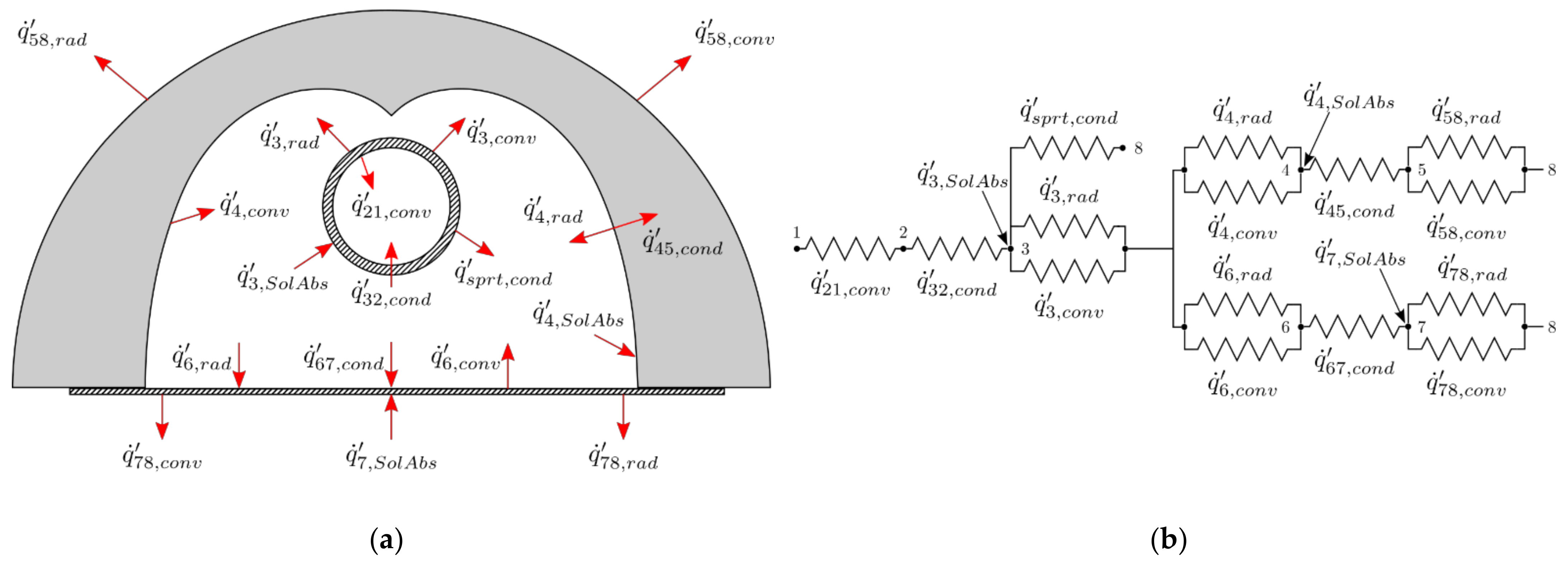
4. Thermo-Hydraulic Model Description and Validation

The thermo-hydraulic model is adapted as described by other researchers [15,32] to the Adiutori methodology [21], as described in previous work [33], and discussed below. Figure 5a shows a schematic of the heat fluxes involved in the surfaces of the receiver. Figure 5b shows the interaction of the involved fluxes in a thermal resistance model equivalent to the heat transfer in the receiver cavity. All the terms in Figure 5 are defined in

Table 5. Definition of heat fluxes in the cavity.

Heat Flux (W/m)	Heat Transfer Mode	Heat Transfer Path
		from	to
${{\dot{q}}^{\prime }}_{21,conv}$	Convection	Inner absorber tube	Heat transfer fluid
${{\dot{q}}^{\prime }}_{32,cond}$	Conduction	Outer absorber tube	Inner absorber tube
${{\dot{q}}^{\prime }}_{spt,cond}$	Conduction	Outer absorber tube	HCE supports
${{\dot{q}}^{\prime }}_{3,SolAbs}$	Absorption of solar radiation	Incident solar radiation	Outer absorber tube
${{\dot{q}}^{\prime }}_{3,rad}$	Radiation	Outer absorber tube	Cavity
${{\dot{q}}^{\prime }}_{3,conv}$	Convection	Outer absorber tube	Cavity
${{\dot{q}}^{\prime }}_{4,rad}$	Radiation	CPC surface	Cavity
${{\dot{q}}^{\prime }}_{4,conv}$	Convection	CPC surface	Cavity
${{\dot{q}}^{\prime }}_{4,SolAbs}$	Absorption of solar radiation	Incident solar radiation	CPC surface
${{\dot{q}}^{\prime }}_{45,cond}$	Conduction	CPC surface	Insulation
${{\dot{q}}^{\prime }}_{58,rad}$	Radiation	Insulation	Environment
${{\dot{q}}^{\prime }}_{58,conv}$	Convection	Insulation	Environment
${{\dot{q}}^{\prime }}_{6,rad}$	Radiation	Inner Pyrex surface	Cavity
${{\dot{q}}^{\prime }}_{6,conv}$	Convection	Inner Pyrex surface	Cavity
${{\dot{q}}^{\prime }}_{67,cond}$	Conduction	Inner Pyrex surface	Outer Pyrex surface
${{\dot{q}}^{\prime }}_{7,SolAbs}$	Absorption of solar radiation	Incident solar radiation	Outer Pyrex surface
${{\dot{q}}^{\prime }}_{78,rad}$	Radiation	Outer Pyrex surface	Environment
${{\dot{q}}^{\prime }}_{78,conv}$	Convection	Outer Pyrex surface	Environment

.

The thermal energy equations were determined by balancing the energy at each surface of the cross-section of the receiver cavity according to the resistance thermal model in Figure 5b and are given below by Equations (1)–(6). Equation (7) was added to balance the change in enthalpy of the HTF as it flows through the absorber tube.

$${{\dot{q}}^{\prime }}_{21,conv}={{\dot{q}}^{\prime }}_{32,cond},$$

(1)

$${{\dot{q}}^{\prime }}_{3,SolAbs}={{\dot{q}}^{\prime }}_{32,cond}+{{\dot{q}}^{\prime }}_{3,rad}+{{\dot{q}}^{\prime }}_{3,conv}+{{\dot{q}}^{\prime }}_{spt,cond},$$

(2)

$${{\dot{q}}^{\prime }}_{45,cond}={{\dot{q}}^{\prime }}_{4,SolAbs}+{{\dot{q}}^{\prime }}_{4,rad}+{{\dot{q}}^{\prime }}_{4,conv},$$

(3)

$${{\dot{q}}^{\prime }}_{45,cond}={{\dot{q}}^{\prime }}_{58,rad}+{{\dot{q}}^{\prime }}_{58,conv},$$

(4)

$${{\dot{q}}^{\prime }}_{67,cond}={{\dot{q}}^{\prime }}_{6,rad}+{{\dot{q}}^{\prime }}_{6,conv},$$

(5)

$${{\dot{q}}^{\prime }}_{7,SolAbs}+{{\dot{q}}^{\prime }}_{67,cond}={{\dot{q}}^{\prime }}_{78,rad}+{{\dot{q}}^{\prime }}_{78,conv},$$

(6)

$${{\dot{q}}^{\prime }}_{21,conv}=\frac{\dot{m}}{L_{HCE}}\left(h_{1out}-h_{1in}\right),$$

(7)

4.1. Solar Absorption

Although the solar radiation fluxes in opaque (such as the absorber) and semi-transparent materials (such as the glass cover) are volumetric phenomena, most of the absorption in the absorber occurs very close to the surface (approximately 6 Å) [34,35], and although solar absorption occurs throughout the thickness of the glass envelope, the absorptivity is relatively small (even for polarized radiation incident at a large angle [36]). These terms can be calculated as:

$${{\dot{q}}^{\prime }}_{3,SolAbs}={\tau }_{67}{\rho }_4{\alpha }_{23}{{\dot{q}}^{\prime }}_{inc,rec},$$

(8)

$${{\dot{q}}^{\prime }}_{4,SolAbs}={\tau }_{67}{\alpha }_{45}{{\dot{q}}^{\prime }}_{inc,rec},$$

(9)

$${{\dot{q}}^{\prime }}_{7,SolAbs}={\alpha }_{67}{{\dot{q}}^{\prime }}_{inc,rec},$$

(10)

where ${\tau }_{67}=0.967$, ${\rho }_4=0.97$, ${\alpha }_{23}=0.94$, ${\alpha }_{45}=0.03$, and ${\alpha }_{67}=0.035$. The incident solar radiation into the receiver (${{\dot{q}}^{\prime }}_{inc,rec}$) takes into account the reflectivity of the primary mirrors and the IAM. The optical parameters are: $\tau$ for the transmittance, $\alpha$ for absorptivity, and $\rho$ for reflectivity of each surface as defined in Table 5.

4.2. Convective Heat Fluxes

To calculate the heat transfer by convection between the three internal surfaces of the cavity, there is no direct methodology due to the geometry, which involves the relationship between unconventional surfaces; however, using a series of dimensionless groups it is possible to apply it to a great variety of cases with pertinent modifications.

The cavity is approximated as two concentric cylinders, as done by Veynandt [32], modyfing the Raithby and Hollands correlation [37], to define the convection for the surfaces (3: outer tube, 4: CPC surface, and 6: inner window) as:

$${{\dot{q}}^{\prime }}_{i,conv}=f\left(\mathrm{Ra}, \mathrm{Pr}\right)\left(T_i-T_c\right),$$

(11)

where $f\left(\mathrm{Ra}, \mathrm{Pr}\right)$ is the corrected Raithby and Hollands correlation to the average cavity temperature $T_c$ as defined by Veynandt [32]. The convection ${{\dot{q}}^{\prime }}_{58,conv}$ can be determined by the Churchill and Chu correlation [38] for free-convection, and for forced convection, the Churchill and Bernstein [39] or Žukauskas [40] correlation can be used. The convection ${{\dot{q}}^{\prime }}_{78,conv}$ can be estimated with McAdams correlation for free-convection, and Pohlhausen [41] or Chilton and Colburn [42] correlations for forced convection.

Internal convection (${{\dot{q}}^{\prime }}_{21,conv}$) is divided into two zones (involving the three fluid regimes): For single-phase fluids, the Gnielinski correlation is applied [42], and the Gungor and Winterton [43] correlation for the two-phase fluid.

4.3. Radiation Heat Fluxex

The radiation heat fluxes in the cavity are determined with the radiosity and the view factors for each surface (3: outer tube, 4: CPC surface, and 6: inner window) as:

$${{\dot{q}}^{\prime }}_{i,rad}={\epsilon }_i\sigma T_i^4+\left(1-{\epsilon }_i\right){\sum }_j{J}_j{F}_{i-j},$$

(12)

where ${\epsilon }_i$ is the emissivity, $T_i$ is the surface temperature, $J_j$ is the radiosity and $F_{i-j}$ is the view factor determined by the geometry of each surface ($F_{3-6}=0.2962$, $F_{3-4}=0.7038$, $F_{4-3}=0.9036$, $F_{4-6}=0.0964$, $F_{6-4}=0.1814$, $F_{6-3}=0.8186$). For the ${{\dot{q}}^{\prime }}_{58,rad}$ and ${{\dot{q}}^{\prime }}_{78,rad}$, the Stefan-Boltzmann equation is applied.

4.4. Conduction Heat Fluxes

Except for ${{\dot{q}}^{\prime }}_{spt,cond}$, which is modelled as a semi-infinite fin [44], all the terms are calculated with the appropriate Fourier equation for conduction (plane and circular wall).

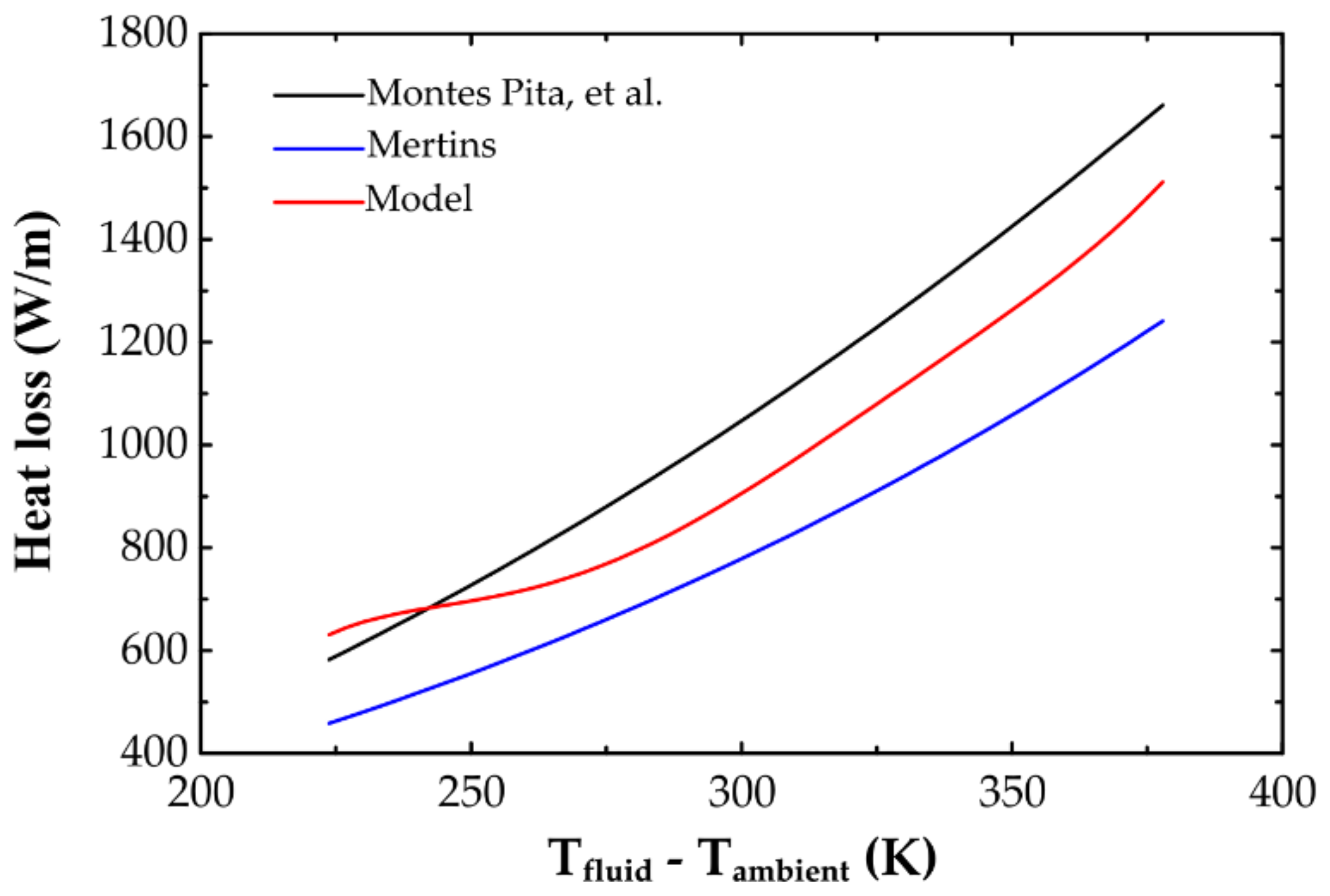
4.5. Thermal Model Validation

Although there are seven balance equations, the model consists of 29 Equations and 29 unknowns grouped into the final seven equations of Equations (1)–(7). The seven groups are defined below:

• Group 1: four solar absorption equations (${{\dot{q}}^{\prime }}_{3,SolAbs}$, ${{\dot{q}}^{\prime }}_{4,SolAbs}$, ${{\dot{q}}^{\prime }}_{5,SolAbs}$, ${{\dot{q}}^{\prime }}_{7,SolAbs}$).
• Group 2: four conduction equations (${{\dot{q}}^{\prime }}_{32,cond}$, ${{\dot{q}}^{\prime }}_{spt,cond}$, ${{\dot{q}}^{\prime }}_{45,cond}$, ${{\dot{q}}^{\prime }}_{67,cond}$).
• Group 3: six convection equations (${{\dot{q}}^{\prime }}_{21,conv}$, ${{\dot{q}}^{\prime }}_{3,conv}$, ${{\dot{q}}^{\prime }}_{4,conv}$, ${{\dot{q}}^{\prime }}_{58,conv}$, ${{\dot{q}}^{\prime }}_{6,conv}$, ${{\dot{q}}^{\prime }}_{78,conv}$).
• Group 4: five radiation equations (${{\dot{q}}^{\prime }}_{3,rad}$, ${{\dot{q}}^{\prime }}_{4,rad}$, ${{\dot{q}}^{\prime }}_{58,rad}$, ${{\dot{q}}^{\prime }}_{6,rad}$, ${{\dot{q}}^{\prime }}_{78,rad}$).
• Group 5: three radiosity equations.
• Group 6: seven balances (one per node).
• Group 7: fluid balance to calculate the enthalpy increase of the fluid.

To solve the non-linear model, the methodology proposed by Adiutori [21] was used to directly solve the temperatures and heat fluxes instead of an iterative method. With this methodology, the convective coefficients are transformed by the functional relations of the heat flow and temperatures, so solving by iterative methods was avoided, resulting in a fast computation with an appropriate convergence with high accuracy [21,45,46]. However, this does not exclude the numerical solution to each heat collection element (HCE) of 5.88 m [33].

To validate the model, the analysis parameters from Montes et al. [15] were tested, and the system of equations was solved to obtain the temperatures and heat fluxes involved in the receiver. The results were compared with the thermal losses of the FRESDEMO field determined by Montes et al. [15] and Mertins [47], as shown in Figure 6. The thermal losses of the proposed model were in between those obtained by Montes et al. [15] and Mertins [47], which demonstrated its validation. At the beginning of the loop, the proposed model showed a greater heat loss than those of Montes et al. [15] and Mertins [47]. This variation is because the present model considered the heat losses associated with the first support placed at the beginning of the loop. However, the error in this zone was less than 5%.

5. Thermo-Hydraulic Performance and Characterization of the System

Once the thermo-hydraulic model was validated, it was directly applied to a case study to establish the lengths of the loops comprising the solar field and to evaluate the energy and exergy efficiencies of the loops. Three characteristic simulation days were chosen: the design day (21 June), the day with the greatest insolation (21 May), and the day with the lowest insolation (21 September). Thus, the results could be generalized to any day of the year; the efficiency lay between the limits of the highest and lowest insolation. The software Meteonorm [48] was used to establish the initial climatological conditions for the model, which are summarized in

Table 6. Weather conditions for Agua Prieta, Sonora.

Parameter	21 June	21 May	21 September
Condition	Design day	Greatest insolation	Lowest insolation
Day of the year	172	141	264
Atmospheric pressure(bar)	0.886	0.884	0.885
Ambient temperature (K)	300.05	295.95	296.95
Effective sky temperature (K)	271.95	265.75	277.75
DNI (W/m2)	856.4815	889.6396	628.8580
Wind speed (m/d)	4	4.1	3.2

.

The simulations were divided into two groups corresponding to the two configurations of the power block described in Section 2. Both cycles were designed to obtain the same net power output (10 MW); however, the number of extractions, mass flow rate, and inlet temperature of the working fluid were modified. Varying these parameters affected the solution of the heat transfer model. Note that the usual operation mode of solar plants is recirculation, where an intermediate water/steam separator is between the preheating and superheating boiling zones [49]. In the present study, the once-through mode was adopted because the scope was limited to determine the thermal behavior of the system.

To solve the model, the mass flow needed to be divided into $N$ loops. The mass flow could not exceed 4.5 kg/s for each loop so that the HTF velocity is approximately the same as in PTC [15]. Thus, different configurations for the solar field can be determined depending on the number of loops that are used, which will affect the total length of the field [4]. The two-steam extraction cycle requires a total mass flow of 12.81 kg/s. Under this restriction, three loops of 4.27 kg/s and four loops of 3.20 kg/s are considered. The three-steam extraction cycle requires a total mass flow of 13.26 kg/s, so three loops of 4.42 kg/s and four loops of 3.32 kg/s are considered.

Therefore, each case was analyzed by considering three and four loops to ensure an adequate mass flow according to the specified limits. Figure 7 shows a diagram of the analysis cases, which resulted in a total of 12 simulations.

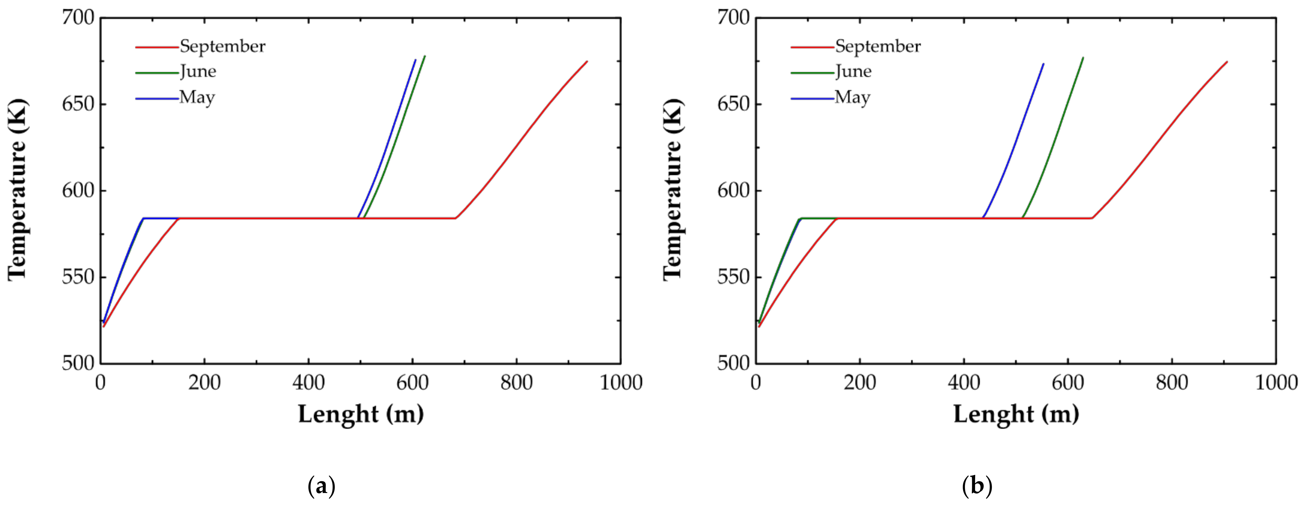
5.1. Three Loops Solar Fields

Figure 8 graphs the required lengths of the loops to heat steam up to 673.15 K on the three analyzed days for two steam extractions (Figure 8a) and for three steam extractions (Figure 8b).

Table 7. Three loop LFR solar field.

Section	Two Steam Extractions			Three Steam Extractions
	June	May	September	June	May	September
Pre-heating (m)	88.6	86.6	161.4	91.5	89.4	156.1
Evaporation (m)	423.9	408.1	479.8	456.6	425.7	533.4
Superheating (m)	111	105.6	264.7	119.5	111	245.9
Length per loop (m)	623.5	600.2	905.9	667.6	626.1	935.5
Total length 1 (km)	1.87	1.8	2.7	2	1.9	2.8

¹: Since the solar field consists of three loops, the total length is multiplied by 3.

summarizes the size of each section of the solar field.

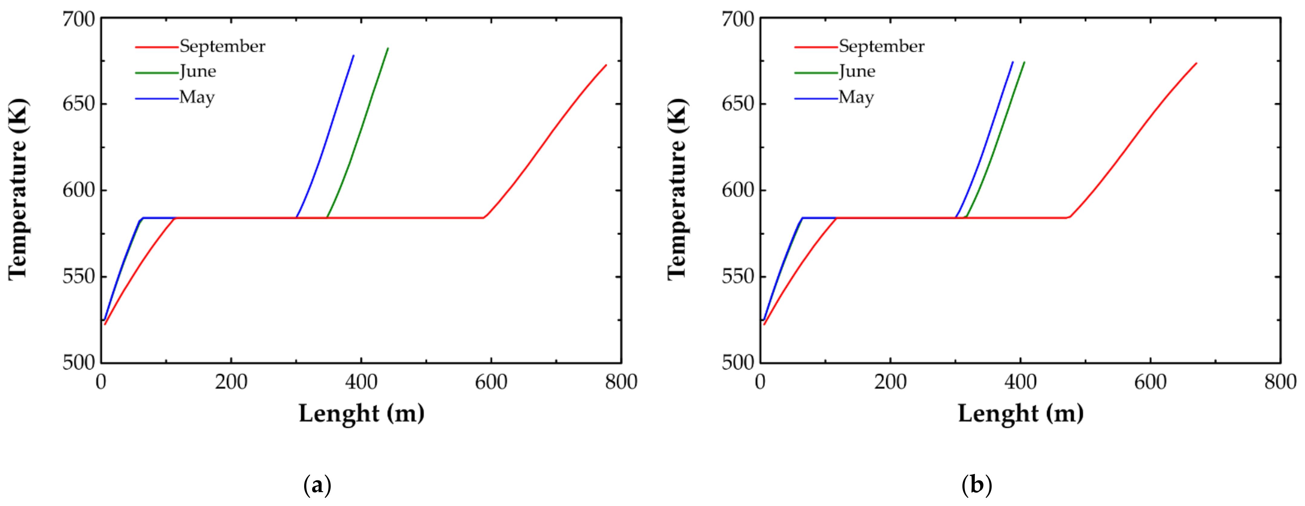
5.2. Four Loops Solar Fields

Figure 9 graphs the required lengths of the loops to heat steam up to 673.15 K on the three analyzed days for two steam extractions (Figure 9a) and for three steam extractions (Figure 9b).

Table 8. Three loop LFR solar field.

Section	Two Steam Extractions			Three Steam Extractions
	June	May	September	June	May	September
Pre-heating (m)	68.4	66.8	119.3	70.5	68.9	123.3
Evaporation (m)	274.8	239.6	476	247	233.8	353.1
Superheating (m)	93.8	81.8	181.1	83.9	81.2	190.3
Length per loop (m)	437	1.6	776.5	401.4	383.9	667.7
Total length 1 (km)	1.7	1.6	3.1	1.6	1.5	2.7

¹: Since the solar field consists of four loops, the total length is multiplied by 4.

summarizes the size of each section of the solar field.

5.3. Dimensions of the Solar Field Loops

The previous Figures show that the longest solar field was on 21 September because this day had the lowest insolation. This was defined as the minimum required length so that the solar plant can deliver the thermal power output required by the power block through the year and continuously operate under nominal conditions (i.e., design point). An important parameter associated with the size of the solar field and power output under nominal operating conditions is the ratio between the average real use and available capacity [49,50]. This ratio gives an idea of how oversized the solar field is relative to the power block and is known as the solar multiple. This is defined as the thermal power supplied by the solar field divided by the thermal power required by the power block to work under nominal conditions:

$$SM=\frac{{\dot{Q}}_{th, solar field}}{{\dot{Q}}_{th,power block}}$$

(13)

A solar multiple greater than unity can be chosen so that the turbine operates under stationary conditions for a longer time interval rather than if the field were sized to the required thermal power at a single point. Figure 10 shows the relationship between thermal power and time for the design and indicates the possible incorporation of an energy storage system.

5.4. Solar Field for a Two-Steam Extraction Regenerative Rankine Cycle Power Block

A solar field with three loops required a length of 935.5 m per loop (total length of 2.8 km), which implies a total concentration area ($A_{pm}$) of 0.059 km². Similarly, for a solar field with four loops required 776.5 m per loop (total length of 3.1 km), which implies a total concentration area of 0.065 km². Figure 11 shows schematic images of the condition.

5.5. Solar Field for a Three-Steam Extraction Regenerative Rankine Cycle Power Block

A solar field with three loops required a length of 905.9 m per loop (total length of 2.7 km), which implies a total concentration area of 0.057 km². Similarly, a solar field with four loops required 776.5 m per loop (total length of 3.1 km), which implies a total concentration area of 0.065 km². Figure 12 shows schematic images of the condition.

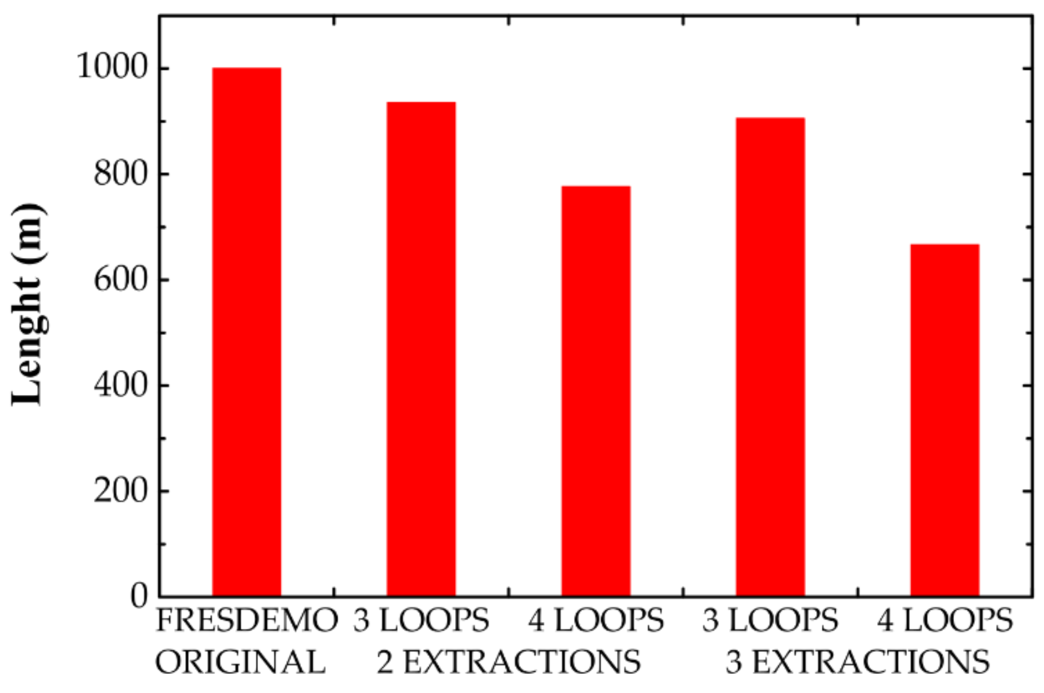
5.6. Solar Field Layout and Length

A shorter pipe system requires fewer of the elements discussed above. In general, a solar field has two possible configurations: the ‘H’ configuration (where the solar field is divided into four sections (north east, north west, south east, and south west) with the power block positioned in the center) for fields with a concentration area of greater than 400,000 m² (0.4 km²), and the ‘I’ configuration (where the solar field is divided into two sections (east and west) with the power block located in the center) for fields with a concentration area of less than 400,000 m² (0.4 km²) [4,49]. The length of each loop for the FRESDEMO field was limited to 1000 m. Together with that of mass flow, this restriction delimited the number of loops required by the solar field.

Simulations with three and four loops for September obtained maximum lengths of 935.5 m and 776.5 m, respectively, for two extractions. Similarly, maximum lengths of 905.9 m and 666.7 m, respectively, were obtained for three extractions. These were chosen as the design configurations, and the solar multiple was determined for the days with the greatest insolation, as summarized in

Table 9. Solar multiple.

Case	Two Steam Extractions			Three Steam Extractions
	June	May	September	June	May	September
Three loops	1.262	1.272	1	1.235	1.251	1
Four loops	1.269	1.277	1	1.251	1.253	1

.

In all cases, the solar multiple was not as excessive for systems without energy storage as reported in the literature, which makes these configurations acceptable, even though the dispatchability of energy is limited by the transient conditions, further studies must be carried out to determine the size and configuration of TES. As the field was relatively small, the loops were arranged in the ‘I’ configuration. Figure 13 compares the decreases in the loop length with the optical optimization.

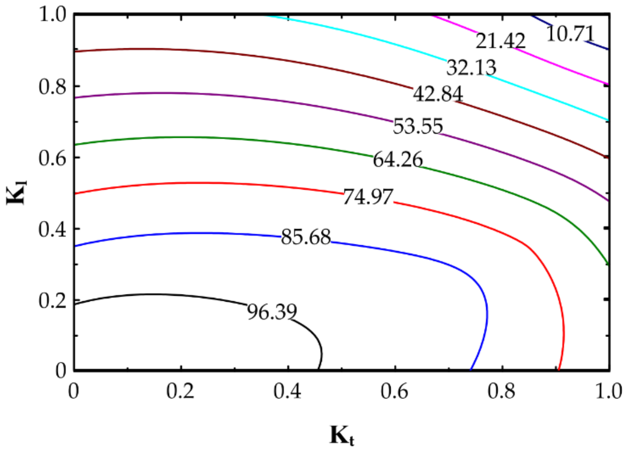
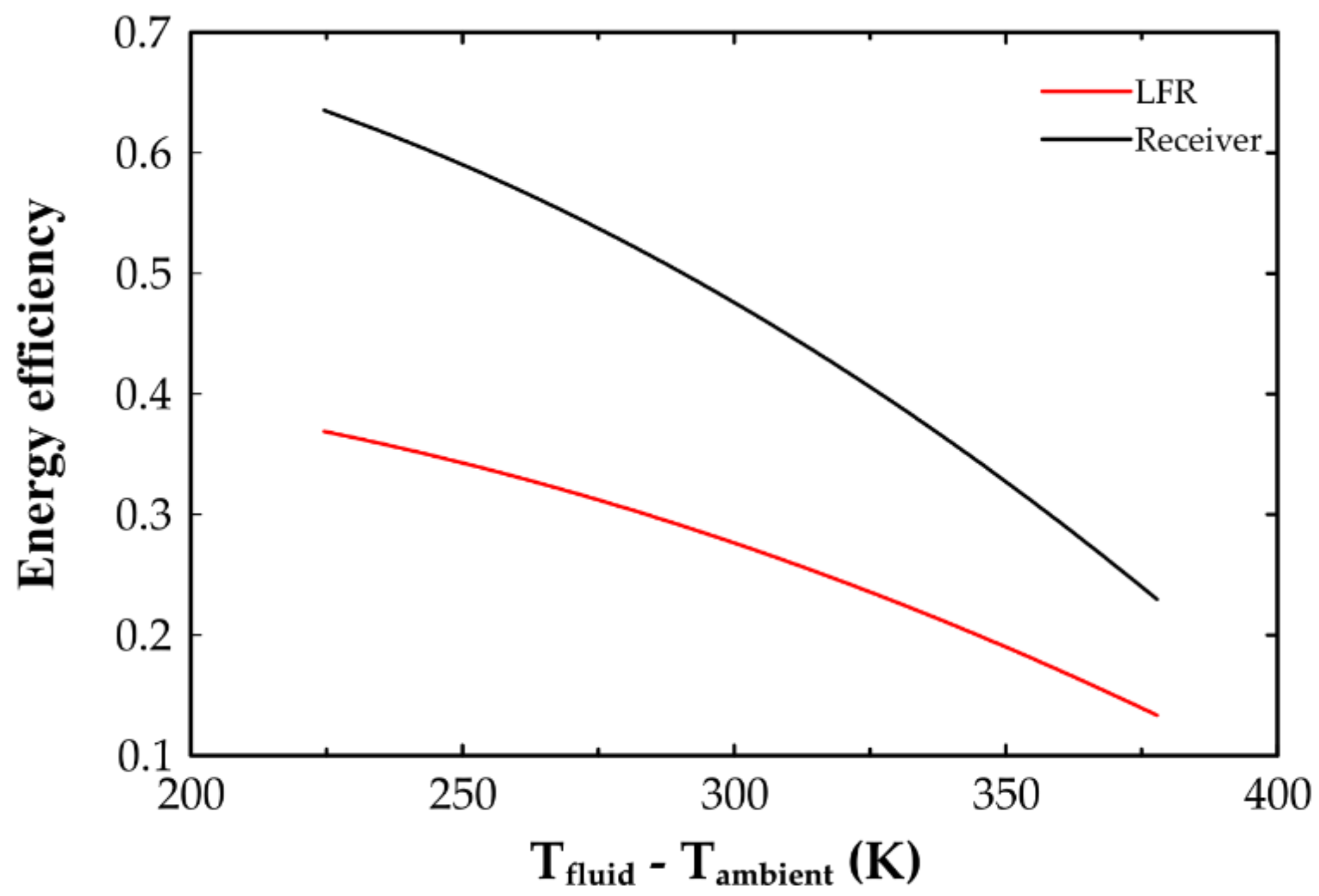
5.7. Energy and Exergy Efficiency

Once the loop length was determined, the energy and exergy efficiency were calculated for the receiver and whole LFR with Equations (14)–(17).

$${\eta }_{I,rec}=\frac{{\dot{Q}}_{HTF}}{{\dot{Q}}_{rec}}$$

(14)

$${\eta }_{I,LFR}=\frac{{\dot{Q}}_{HTF}}{{\dot{Q}}_{PM}}$$

(15)

$${\eta }_{II,rec}=\frac{{\dot{B}}_{HTF}}{{\dot{B}}_{rec}}$$

(16)

$${\eta }_{II,LFR}=\frac{{\dot{B}}_{HTF}}{{\dot{B}}_{PM}}$$

(17)

where ${\dot{Q}}_{HTF}$ is the heat gain rate of the HTF, ${\dot{Q}}_{rec}$ is the heat rate impinging the receiver, ${\dot{Q}}_{PM}$ is the heat rate captured by the primary mirrors, ${\dot{B}}_{HTF}$ is the exergy heat gain rate of the HTF, ${\dot{B}}_{rec}$ is the heat exergy rate impinging the receiver, and ${\dot{B}}_{PM}$ is the radiative exergy rate captured by the primary mirrors according to Parrot’s formulation [51].

The thermal efficiency analysis of the receiver and concentrator showed a significant decrease in efficiency after the phase change. In the first HCE, the efficiencies of the concentrator and receiver were 0.37 and 0.63, respectively; at the exit of the loop, these fall to 0.14 and 0.24, respectively. This decrease in energy efficiency is shown in Figure 14.

The exergy efficiency of the receiver behaved differently compared to the energy efficiency, but the exergy efficiency of the concentrator did not, as shown in Figure 15. This is because the energy efficiency decreases with an increased working temperature because of the increased heat loss, while the exergy efficiency increases with temperature but not as much at higher temperatures. In the first HCE, the exergy efficiencies of the concentrator and receiver were 0.60 and 0.14, respectively; at the exit of the loop, these became 0.23 and 0.19, respectively.

Figure 16a graphs the increase in heat loss per unit length against the difference in temperature between the fluid and environment. The heat losses increased too much once the superheated steam regime was reached. The pressure drop showed similar behavior (Figure 16b). In the superheated steam regime, the pressure loss became more evident and reached close to 0.1 bar.

With the computation of heat loss (Figure 16a) and pressure drop (Figure 16b) across the solar field, an important observation can be formulated comparing these two parameters. Bejan [22,52] has proposed the irreversibility distribution ratio, Equation (18), while Paoletti [53] defined the Bejan number, Equation (18), as dimensionless groups to compare the irreversibility between heat transfer and pressure drop. Alternatively, instead of the entropy generation terms in Equations (18) and (19), exergy destruction terms can be considered as shown, where the meaning of $\varphi$ and $\mathrm{Be}$ remains the same.

$$\varphi =\frac{{{\dot{S}}^{\prime }}_{gen,\mathsf{\Delta }p}}{{{\dot{S}}^{\prime }}_{gen,{\dot{Q}}_l^{\prime }}}=\frac{{\dot{B}}_{dest,\mathsf{\Delta }p}}{{\dot{B}}_{dest,{\dot{Q}}_l^{\prime }}}$$

(18)

$$\mathrm{Be}={\left(1+\varphi \right)}^{-1}$$

(19)

Accordingly, it can be concluded that when $\mathrm{Be}\to 1$, the heat transfer irreversibility dominates, while when $\mathrm{Be}\to 0$ the irreversibility is dominated by the pressure drop. The exergy destruction by heat loss and pressure drop can be quantified by:

$${\dot{B}}_{dest,\mathsf{\Delta }p}=T_{amb}\frac{1}{T_1}\frac{\dot{m}}{\rho }\mathsf{\Delta }p$$

(20)

$${\dot{B}}_{dest,{\dot{Q}}_l}=T_{amb}\frac{1}{T_1}{\dot{Q}}_l^{\prime }$$

(21)

where $T_{amb}=300 \mathrm{K}$ is the ambient temperature, $T_1$ is the HTF temperature, $\dot{m}$ is the mass flow rate, $\mathsf{\Delta }p$ is the pressure drop, and ${\dot{Q}}_l^{\prime }$ is the heat loss rate. For the optimized field, $\mathrm{Be}=0.9975$, so the heat losses dominate the irreversibilities across the solar field.

5.8. Comparison of the Optimized Field and FRESDEMO

With the previous data, a comparison regarding the 2E analysis performed on the optimized field and the reported values for FRESDEMO by Montes et al. [15] is described in

Table 10. Comparison of 2E analysis between FRESDEMO [15] and the optimized field.

Parameter	FRESDEMO	Optimized Field
Energy efficiency	67%	64%
Exergy efficiency	63%	60%
Bejan number	0.9901 1	0.9975
Maximum length (m)	1000	935
Maximum SM	−	1.27

¹: This parameter was not determined by Montes et al. [15], but determined with the reported data.

.

6. Conclusions

A novel study of the design of a solar power plant is discussed. The solar plant can supply the required thermal power through a regenerative Rankine cycle with two and three steam extractions. The power cycles were determined under the assumption that the exergetic efficiency of the entire system should be optimized, which implies that the largest amount of useful energy can be used. Thus, a sensibility analysis was performed to optimize the extraction pressures of the turbine to minimize the total destroyed exergy.

Once the required thermal power output of the solar field was determined, the number of loops was established for power cycles with two and three steam extractions considering the maximum (4.5 kg/s) and minimum mass flows (2 kg/s) of LFRs plants. Two alternatives were considered for each case: three and four loops. The analysis was performed for the average day (21 June), day of greatest insolation (21 May), and day of lowest insolation (21 September), to determine both the surface temperature and length of each loop applying Adiutori’s methodology [21] to solve the thermal model.

The length of each loop was limited to the length of the FRESDEMO field (1000 m). This restriction together with the mass flow restriction delimited the number of loops required by the solar field. The simulation results showed that the maximum loop length for three and four loops on 21 September was 905.9 m and 776.5 m, respectively, for two extractions, and 935.5 m and 667.6 m, respectively, for three extractions. As stated above, it was expected that using an optically optimized field would reduce the length of the loops. Under the cases analyzed, the decrease in length varies from 6.45% to 33.3%; while keeping a solar multiple between 1.25 and 1.27.

These were chosen as the design configurations, and the solar multiple was determined for the day with the highest insolation. In all cases, the solar multiple did not exceed that for systems without energy storage as reported in the literature. Thus, these configurations are ideal for future implementation.

Contrary to what is thought, when a concentration system is optically optimized, thermal efficiency is negatively affected [50,54]. Comparing the results of the optimized Field with FRESDEMO [15], the optimized field presents an increase in optical efficiency of 28%, resulting in thermal efficiency decreases of less than 5%; with the advantage that the length of the loop has decreased; while the irreversibility across the solar field presents a similar behavior between the pressure drop and the heat loss.

When comparing the decrease in thermal efficiency against the decrease in the length of the loop, it may be beneficial to sacrifice a little thermal efficiency since the system costs would go down. Future studies could fruitfully explore this issue further by comparing the behavior of the optimized Fresnel reflector and a parabolic through solar field in order to establish a criterion for future implementation.

References

1. BP. Statistical Review of World Energy. 2018. Available online: https://www.bp.com/en/global/corporate/energy-economics/statistical-review-of-world-energy.html (accessed on 15 February 2019).
2. Bernhard, R.; Laabs, H.-J.; de LaLaing, J.; Eickhoff, M. Linear Fresnel Collector Demonstration on the PSA, Part I—Design, Construction and Quality Control. In Proceedings of the International Symposium on Concentrated Solar Power and Chemical Energy Technologies, Casablanca, Morroco, 2–5 October 2008; Available online: https://www.researchgate.net/publication/225000351_Linear_Fresnel_Collector_Demonstration_on_the_PSA_Part_I_-_Design_Construction_and_Quality_Control (accessed on 10 July 2021).
3. González-Mora, E.; Durán García, M.D. Methodology for an Opto-Geometric Optimization of a Linear Fresnel Reflector for Direct Steam Generation. Energies 2020, 13, 355. [Google Scholar] [CrossRef] [Green Version]
4. Montes Pita, M.J. Análisis Y Propuestas De Sistemas Solares De Alta Exergía Que Emplean Agua Como Fluido Calorífero. Ph.D. Thesis, Universidad Politécnica de Madrid, Madrid, Spain, 2008. [Google Scholar]
5. Almanza, R.; Lentz, A. Electricity production at low powers by direct steam generation with parabolic troughs. Sol. Energy 1998, 64, 115–120. [Google Scholar] [CrossRef]
6. Almanza, R.; Lentz, A.; Jiménez, G. Receiver behavior in direct steam generation with parabolic troughs. Sol. Energy 1997, 61, 275–278. [Google Scholar] [CrossRef]
7. Cui, W.; Li, H.; Li, L.; Liao, Q. Thermal stress analysis of DSG solar absorber tube in stratified two-phase regime. AIP Conf. Proc. 2013, 1558, 2217–2220. [Google Scholar]
8. Eck, M.; Zarza, E.; Eickhoff, M.; Rheinländer, J.; Valenzuela, L. Applied research concerning the direct steam generation in parabolic troughs. Sol. Energy 2003, 74, 341–351. [Google Scholar] [CrossRef]
9. Zarza Moya, E. Generación Directa de Vapor con Colectores Solares Cilindro Parabólicos. Proyecto DIrect Solar Steam (DISS). Ph.D. Thesis, Universidad de Sevilla, Sevilla, Spain, 2003. [Google Scholar]
10. IEA. Technology Roadmap-Solar Thermal Electricity; IEA: Paris, France, 2014.
11. NREL. Concentrating Solar Power Projects. Available online: https://solarpaces.nrel.gov/ (accessed on 20 March 2020).
12. IRENA. Solar Energy. Available online: https://www.irena.org/solar (accessed on 27 February 2021).
13. Elsafi, A.M. Exergy and exergoeconomic analysis of sustainable direct steam generation solar power plants. Energy Convers. Manag. 2015, 103, 338–347. [Google Scholar] [CrossRef]
14. Schenk, H.; Hirsch, T.; Fabian Feldhoff, J.; Wittmann, M. Energetic comparison of linear Fresnel and parabolic trough collector systems. J. Sol. Energy Eng. 2014, 136, 041015. [Google Scholar] [CrossRef]
15. Montes, M.J.; Barbero, R.; Abbas, R.; Rovira, A. Performance model and thermal comparison of different alternatives for the Fresnel single-tube receiver. Appl. Therm. Eng. 2016, 104, 162–175. [Google Scholar] [CrossRef]
16. Hakkarainen, E.; Tähtinen, M.; Mikkonen, H. Dynamic model development of linear Fresnel solar field. In Proceedings of the ASME 2015 Power and Energy Conference, New York, NY, USA, 2–28 July 2015. [Google Scholar]
17. Giostri, A.; Binotti, M.; Silva, P.; Macchi, E.; Manzolini, G. Comparison of two linear collectors in solar thermal plants: Parabolic trough versus Fresnel. J. Sol. Energy Eng. 2013, 135, 011001. [Google Scholar] [CrossRef]
18. Hirsch, T.; Khenissi, A. A systematic comparison on power block efficiencies for CSP plants with direct steam generation. Energy Procedia 2013, 49, 1165–1176. [Google Scholar] [CrossRef] [Green Version]
19. Sun, J.; Liu, Q.; Hong, H. Numerical study of parabolic-trough direct steam generation loop in recirculation mode: Characteristics, performance and general operation strategy. Energy Convers. Manag. 2015, 96, 287–302. [Google Scholar] [CrossRef]
20. Hakkarainen, E.; Kannari, L. Dynamic Modelling of Concentrated Solar Field for Thermal Energy Storage Integration. In Proceedings of the 9th International Renewable Energy Storage Conference (IRES 2015), Düsseldorf, Germany, 9–11 March 2015. [Google Scholar]
21. Adiutori, E. The New Engineering, 3rd ed.; Ventuno Press: Naples, FL, USA, 2017; ISBN 978-0-9626220-4-5. [Google Scholar]
22. Bejan, A. Entropy Generation Minimization: The Method of Thermodynamic Optimization of Finite-Size Systems and Finite-Time Processes; Mechanical and Aerospace Engineering Series; Taylor & Francis: Boca Raton, FL, USA, 1995; ISBN 978-0-84939-651-9. [Google Scholar]
23. Ying, Y.; Hu, E.J. Thermodynamic advantages of using solar energy in the regenerative Rankine power plant. Appl. Therm. Eng. 1999, 19, 1173–1180. [Google Scholar] [CrossRef]
24. Moran, M.J.; Shapiro, H.N.; Boettner, D.D.; Bailey, M.B. Fundamentals of Engineering Thermodynamics, 8th ed.; Wiley: Hobooken, NJ, USA, 2014; ISBN 978-1-118-41293-0. [Google Scholar]
25. Balmer, R.T. Modern Engineering Thermodynamics, 1st ed.; Academic Press: Cambridge, MA, USA, 2011; ISBN 008-096-1738. [Google Scholar]
26. Siemens. Efficiency Turns Less into More; Siemens: Munich, Germany, 2017. [Google Scholar]
27. Coco-Enríquez, L.; Muñoz-Antón, J.; Martínez-Val, J.M. Innovations on direct steam generation in linear Fresnel collectors. In Proceedings of the SolarPACES2013, Las Vegas, NV, USA, 17–20 September 2013; p. 45721. [Google Scholar]
28. Bejan, A. Advanced Engineering Thermodynamics, 1st ed.; Wiley: Hoboken, NJ, USA, 2016; ISBN 978-0-47090-037-6. [Google Scholar]
29. Bartlett, R.L. Steam Turbine Performance and Economics, 1st ed.; McGraw-Hill: New York, NY, USA, 1958. [Google Scholar]
30. Tabatabaian, M.; Post, S.; Rajput, R.K. Advanced Thermodynamics; Mercury Learning Series; Mercury Learning & Information: Herndon, VA, USA, 2017; ISBN 978-1-93642-027-8. [Google Scholar]
31. Boito, P.; Grena, R. Optimization of the geometry of Fresnel linear collectors. Sol. Energy 2016, 135, 479–486. [Google Scholar] [CrossRef]
32. Veynandt, F. Cogénération Héliothermodynamique avec Concentrateur Linéaire de Fresnel: Modélisation de L’ensemble du Procédé. Ph.D. Thesis, Université de Toulouse, Toulouse, France, 2011. [Google Scholar]
33. González-Mora, E.; Durán García, M.D. Energy and Exergy (2E) Analysis of an Optimized Linear Fresnel Reflector for a Conceptual Direct Steam Generation Power Plant. In Proceedings of the ISES Solar World Congress 2019, Santiago, Chile, 4–7 November 2019; International Solar Energy Society: Freiburg, Germany, 2019; pp. 907–918. [Google Scholar]
34. Özışık, M.N. Radiative Transfer and Interactions with Conduction and Convection, 1st ed.; Wiley: Hoboken, NJ, USA, 1973; ISBN 978-0-47165-722-4. [Google Scholar]
35. Howell, J.R.; Menguc, M.P.; Siegel, R. Thermal Radiation Heat Transfer, 6th ed.; CRC Press: Boca Raton, FL, USA, 2015; Volume 92, ISBN 978-1-49875-774-4. [Google Scholar]
36. Rabl, A. Active Solar Collectors and Their Applications; Oxford University Press: Oxford, UK, 1985; ISBN 978-0-19536-521-4. [Google Scholar]
37. Raithby, G.D.; Hollands, K.G.T. A General Method of Obtaining Approximate Solutions to Laminar and Turbulent Free Convection Problems. Adv. Heat Transf. 1975, 11, 265–315. [Google Scholar]
38. Churchill, S.W.; Chu, H.H.S. Correlating equations for laminar and turbulent free convection from a horizontal cylinder. Int. J. Heat Mass Transf. 1975, 18, 1049–1053. [Google Scholar] [CrossRef]
39. Churchill, S.W.; Bernstein, M. A Correlating Equation for Forced Convection From Gases and Liquids to a Circular Cylinder in Crossflow. J. Heat Transf. 1977, 99, 300–306. [Google Scholar] [CrossRef]
40. Žukauskas, A. Heat Transfer from Tubes in Crossflow. Adv. Heat Transf. 1972, 8, 93–160. [Google Scholar]
41. Pohlhausen, E. Der Wärmeaustausch zwischen festen Körpern und Flüssigkeiten mit kleiner reibung und kleiner Wärmeleitung. ZAMM J. Appl. Math. Mech. Z. Angew. Math. Mech. 1921, 1, 115–121. [Google Scholar] [CrossRef] [Green Version]
42. Bergman, T.L.; Lavine, A.S.; Incropera, F.P.; Dewitt, D.P. Fundamentals of Heat and Mass Transfer, 7th ed.; John Wiley & Sons, Inc.: Hoboken, NJ, USA, 2011; ISBN 978-0-47050-197-9. [Google Scholar]
43. Gungor, K.E.; Winterton, R.H.S. A general correlation for flow boiling in tubes and annuli. Int. J. Heat Mass Transf. 1986, 29, 351–358. [Google Scholar] [CrossRef]
44. Forristall, R. Heat Transfer Analysis and Modeling of a Parabolic Trough Solar Receiver Implemented in Engineering Equation Solver; National Renewable Energy Lab.: Golden, CO, USA, 2003. [Google Scholar]
45. Adiutori, E.F. A Critical Examination of Correlation Methodology Widely Used in Heat Transfer and Fluid Flow. In Proceedings of the ASME 2004 Heat Transfer/Fluids Engineering Summer Conference ASMEDC, Charlotte, NC, USA, 11–15 July 2004; Volume 1, pp. 929–934. [Google Scholar]
46. Adiutori, E.F. Why Conventional Engineering Science should be Abandoned, and the New Engineering Science that should Replace It. Am. J. Mech. Eng. 2020, 9, 1–6. [Google Scholar] [CrossRef]
47. Mertins, M. Technische und Wirtschaftliche Analyse von Horizontalen Fresnel-Kollektoren. Ph.D. Thesis, Universität Karlsruhe, Baden-Württemberg, Gremany, 2009. [Google Scholar]
48. Meteotest Meteonorm; Version 7.2; METEOTEST: Bern, Switzerland, 2018.
49. Wang, Z. Design of Solar Thermal Power Plants; Elsevier Science: Amsterdam, The Netherlands, 2019; ISBN 978-0-12815-613-1. [Google Scholar]
50. Lovegrove, K.; Stein, W. Chapter 1-Introduction to concentrating solar power technology. In Concentrating Solar Power Technology; Lovegrove, K., Stein, W.B.T.-C.S.P.T., Eds.; Woodhead Publishing Series in Energy; Woodhead Publishing: Cambridge, UK, 2021; pp. 3–17. ISBN 978-0-12-819970-1. [Google Scholar]
51. Parrott, J.E. Theoretical upper limit to the conversion efficiency of solar energy. Sol. Energy 1978, 21, 227–229. [Google Scholar]
52. Bejan, A. Entropy Generation through Heat and Fluid Flow; Wiley: Hoboken, NJ, USA, 1982; Volume 1, ISBN 0-471-09438-2. [Google Scholar]
53. Paoletti, S.; Rispoli, F.; Sciubba, E. Calculation of exergetic losses in compact heat exchanger passages. In Proceedings of the ASME AES, San Francisco, CA, USA, 10–15 December 1989; Volume 10, pp. 21–29. [Google Scholar]
54. Blanco, M.J.; Miller, S. 1-Introduction to concentrating solar thermal (CST) technologies. In Advances in Concentrating Solar Thermal Research and Technology; Elsevier: Amsterdam, The Netherlands, 2017; pp. 3–25. [Google Scholar]
Figure 1. Regenerative Rankine cycle with two steam extractions: (a) Schematic diagram; (b) T–s diagram.
Energies 14 04234 g001
Figure 2. Regenerative Rankine cycle with three steam extractions: (a) Schematic diagram; (b) T–s diagram.
Energies 14 04234 g002
Figure 3. Incidence angle modifiers for the longitudinal (Kl) and transverse (Kt) directions [3].
Energies 14 04234 g003
Figure 4. Average optical concentration on the receiver plane [3].
Energies 14 04234 g004
Figure 5. Heat transfer model in the cavity in the receiver: (a) Cross section of a single tube Fresnel receiver; (b) Thermal resistance model for single tube Fresnel receiver.
Energies 14 04234 g005
Figure 6. Comparison between the thermal losses calculated by the thermal model of Montes et al. [15]; thermal model of Mertins [47], and proposed model.
Energies 14 04234 g006
Figure 7. Simulation cases.
Energies 14 04234 g007
Figure 8. Water/steam temperature along an LFR with three loops in once-through operation mode: (a) Two steam extractions; (b) Three steam extractions.
Energies 14 04234 g008
Figure 9. Water/steam temperature along an LFR with four loops in once-through operation mode: (a) Two steam extractions; (b) Three steam extractions.
Energies 14 04234 g009
Figure 10. Effects of sizing the solar field with different solar multiples.
Energies 14 04234 g010
Figure 11. Solar multiple for two steam extractions: (a) Three loops; (b) Four loops.
Energies 14 04234 g011
Figure 12. Solar multiple for two steam extractions: (a) Three loops; (b) Four loops.
Energies 14 04234 g012
Figure 13. Comparison of the length of the simulated loops.
Energies 14 04234 g013
Figure 14. Thermal efficiency of the LFR and the receiver.
Energies 14 04234 g014
Figure 15. Exergy efficiency: (a) Receiver; (b) LFR.
Energies 14 04234 g015
Figure 16. General losses in the solar field: (a) Heat loss; (b) Pressure drop.
Energies 14 04234 g016