State-Space Model of Quasi-Z-Source Inverter-PV Systems for Transient Dynamics Studies and Network Stability Assessment

Abstract

Photovoltaic (PV) power systems are increasingly being used as renewable power generation sources. Quasi-Z-source inverters (qZSI) are a recent, high-potential technology that can be used to integrate PV power systems into AC networks. Simultaneously, concerns regarding the stability of PV power systems are increasing. Converters reduce the damping of grid-connected converter systems, leading to instability. Several studies have analyzed the stability and dynamics of qZSI, although the characterization of qZSI-PV system dynamics in order to study transient interactions and stability has not yet been properly completed. This paper contributes a small-signal, state-space-averaged model of qZSI-PV systems in order to study these issues. The model is also applied to investigate the stability of PV power systems by analyzing the influence of system parameters. Moreover, solutions to mitigate the instabilities are proposed and the stability is verified using PSCAD time domain simulations.

1. Introduction

Photovoltaic (PV) systems have become some of the most popular renewable generation sources [1,2,3]. They can have different configurations based on centralized or multiple inverters with single- or two-stage topologies [4,5]. The flexibility and efficiency of two-stage voltage source inverter (VSI) topologies have led to their widespread use; however, single-stage topologies based on impedance-source networks with a centralized inverter [6,7,8,9] or micro-inverters [10,11] are increasing in popularity as simple and economical configurations that can overcome the shortcomings of two-stage VSI topologies. Reviews of single-stage impedance-based converters (including the main topologies, modeling, control and cutting-edge techniques) are presented in [6,7,8]. An analytical comparison of the passive components and semiconductor stress of the previous inverters and multilevel buck–boost inverters is presented in [9]. Single-stage impedance-based converters such Z-source and quasi-Z-source inverters (qZSIs) are currently used for the integration of renewables and grids [6,9]. A review of the use of micro-inverters as a rising technology in PV systems is also presented in [10,11]. In particular, qZSIs are promising because buck–boost voltage is efficiently and reliably generated in a single-stage operation [6,7,8,9,12,13,14,15,16,17]. A traditional qZSI with a semiconductor and impedance network between the DC energy source and the AC grid inverter is investigated in [6,7,8,9,12,13,14]. Four improved qZSIs are theoretically studied in [15], while a three-level NPC qZSI, which provides high energy density, short circuit immunity and voltage regulation (step-down and step-up) capability, is examined in [16,17].

Grid integration of PV power systems can lead to stability problems because the damping of power conversion systems connected to the grid is reduced by power electronics. Many studies have dealt with this issue in PV power systems based on traditional two-stage converter topologies by means of small-signal state-space (SS) models. Specifically, the impacts of PV power system variables (e.g., solar irradiance and temperature [18,19]) and control parameters [3] on stability have been investigated. Other works have looked at qZSI-PV system stability, but most only have provided qZSI dynamic models to analyze qZSI stability and derive general conclusions about qZSI-PV system stability [6,7,8,12,13,14,17]. The qZSI control methods and their influence on qZSI stability are explored in [6,14], while qZSI design guides are given from these dynamic models in [12,13]. Exhaustive operating range studies on the impacts of converter variables on the transient response of different Z-source inverters such as qZSIs are also performed in [7,8]. Moreover, qZSI modeling for analysis of qZSI controls is applied in [17]. It is worth noting that very few studies have provided dynamic models of a complete qZSI-PV system [20,21,22,23,24,25]. Such studies have mainly explored the influence of an AC network on DC-side stability [20,23,24] and qZSI dynamics [21,22]. On the other hand, dynamic interactions between AC and DC networks have not been fully studied yet. Recently, two qZSI-PV system simulation models based on PSCAD and Simulink were introduced in [25], and these dynamic interactions and qZSI-PV system stability were studied from the proposed models; however, these models (and their corresponding studies) are limited by the features of the PSCAD and Simulink tools, and a qZSI-PV system model based on the small-signal state-space equation is required to have more flexibility in the qZSI-PV system dynamic simulations and stability analysis.

This paper extends the work in [25] and contributes a fully developed small-signal state-space averaged (SSA) equation of qZSI-PV systems for implementation in customized codes of time domain simulation and stability studies. The equation is systematically and rigorously obtained by considering the main qZSI-PV system controls, i.e., maximum power point (MPP) tracking (MPPT), PV voltage, grid current and qZSI duty cycle controls. The models in [25] only allow Simulink and PSCAD dynamic studies of qZSI-PV system behavior to be performed, while our model enables the use of different software programs (e.g., Simulink and MATLAB environments), increasing the possibility to carry out qZSI-PV system dynamics studies, such as the following:

• PV system stability studies in the frequency domain;
• Participation factor (PF) assessments and analytical studies of the influence of PV system parameters on stability;
• AC grid-connected PV system dynamics studies based on a single Simulink model of qZSI-PV systems derived from the proposed model.

Here, the contributions to the knowledge of the following stability issues are presented through the application of the proposed equation:

• Impacts of qZSI-PV system parameters on stability;
• Proposals for stability improvement from PFs and analysis of qZSI-PV system damping parameters.

All of these contributions, which are numerically validated by PSCAD simulations, can be used together as a valuable transient modeling tool and in qZSI-PV system stability studies.

2. State-Space Modeling of PV Power Systems

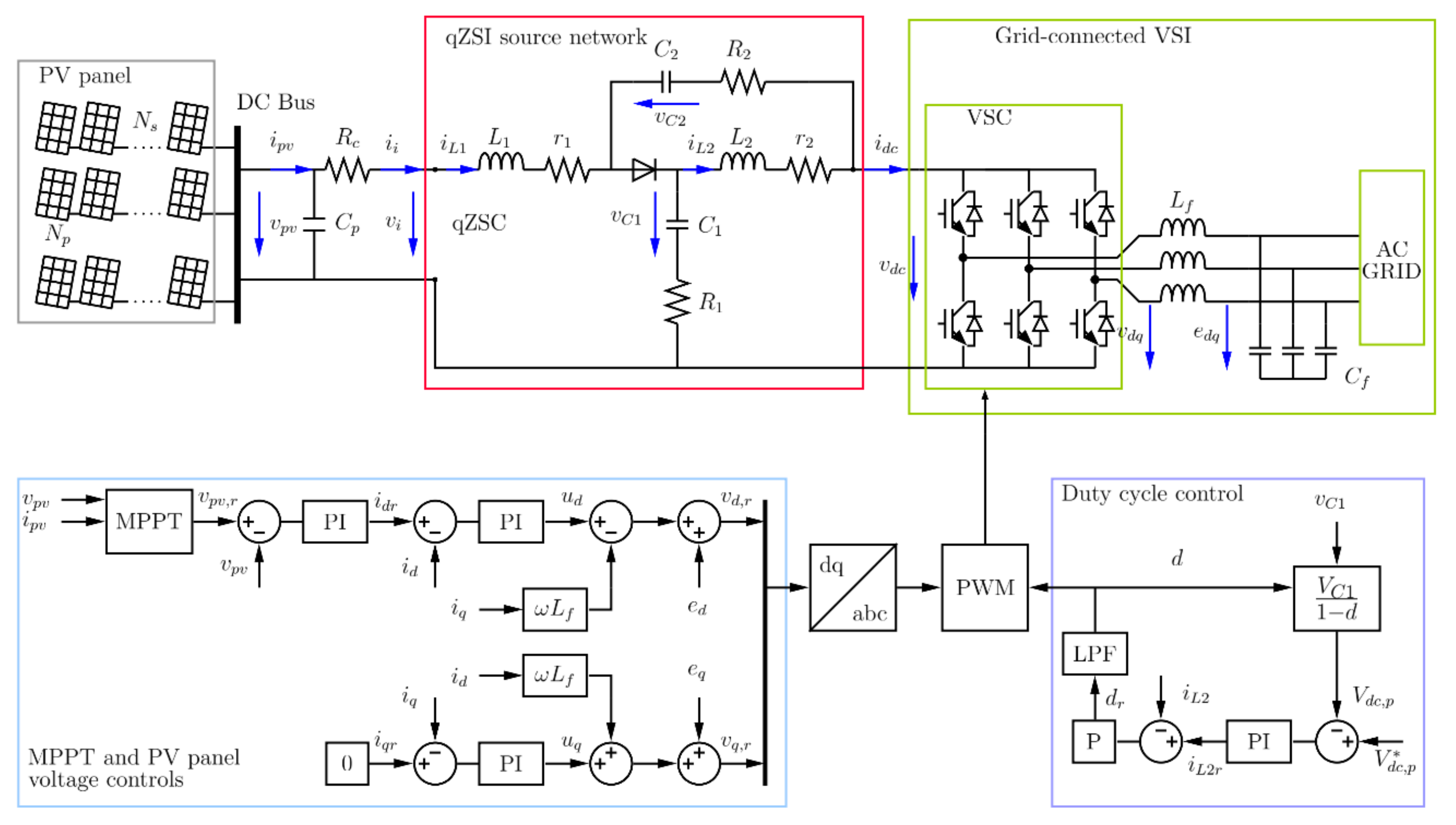
In order to evaluate the qZSI-PV system stability, SSA modeling of the circuit in Figure 1 is presented based on the following state-space equation:

$$\frac{d\mathrm{\Delta }\mathbf{x}}{dt}=A\mathrm{\Delta }x+B_1\mathrm{\Delta }{u}_1+B_2\mathrm{\Delta }{u}_2\hspace{1em}\hspace{1em}\mathrm{\Delta }y=C\mathrm{\Delta }x+E_1\mathrm{\Delta }{u}_1+E_2\mathrm{\Delta }{u}_2,$$

(1)

where x, u₁, u₂ and y are the state, internal input, external input and output vectors, respectively, while the small-signal variables are denoted by the symbol Δ.

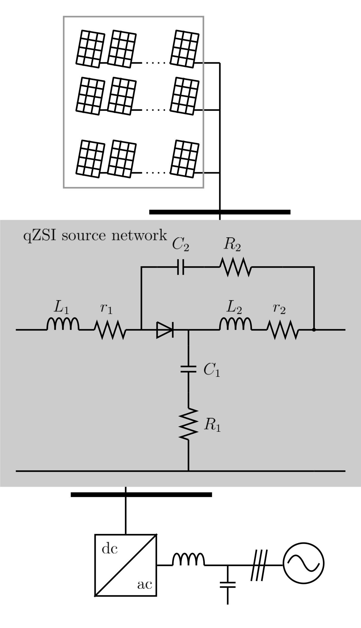
Broadly speaking, qZSI-PV systems have a PV installation supplying the qZSI (i.e., the N_p × N_s PV panel, the capacitor C_p and the DC conductor resistance R_c), which allows the output voltage v_dc to be boosted at the VSI terminals. The N_p × N_s PV panel has N_p strings in parallel with N_s PV cells in series.

To fully extract the PV panel’s maximum power, an MPPT algorithm and the voltage control of the PV panel are used. The VSI current control loop fixes the power that the VSI delivers to the grid. The DC peak voltage v_dc,p is adjusted using the qZSI duty cycle control. The pulse width modulation (PWM) block generates the trigger signals of the IGBTs (i.e., the shoot-through states of the qZSI) from the grid dq-frame reference voltage v_dqr and the duty cycle d by means of the carrier-based sinewave pulse width modulation method, referred to as simple boost control (see Chapter 4 in [6]). The dynamic behavior of the qZSI-PV system components is dictated by their SS equations, while the averaging approach for these equations used for characterizing the two qZSI states is also applied for qZSI modeling. The development of SSA equations is well documented in [25], so only a summary is presented in the following subsections. All qZSI-PV system component equations are turned into a single SSA equation that characterizes the qZSI-PV system dynamics. This equation is validated using PSCAD simulations.

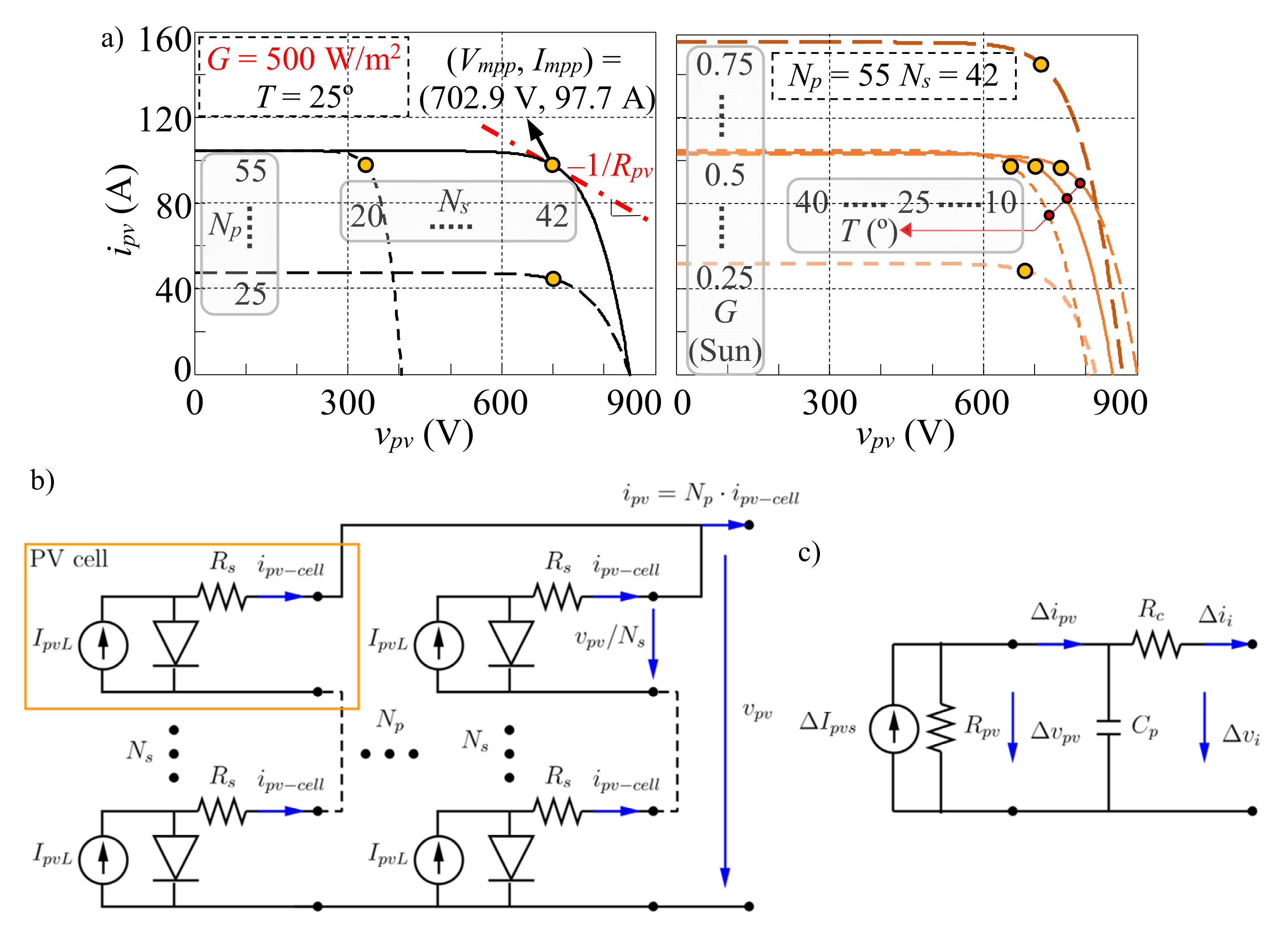
2.1. Model of the PV Installation

The SS equation for the PV installation is presented in this subsection. A typical I–V plot of a PV panel is shown to highlight the different parameter values in Figure 2a, where the MPPs of the different I–V plots are labelled with dots. The panel has an N_p × N_s 60 W PV Solarex MSX60 module (see specifications in [2]). It is noted that for a constant irradiance level G and temperature T, an increase in the number of PV panels in series N_s leads to an increase in the voltage of the PV panel v_pv, while the same is true for the number of PV panels in parallel N_p and the current of the PV panel i_pv. This I–V plot of a PV panel is expressed as [2,4,25]:

$$i_{pv}=N_p\left\{I_{pvL}-I_{pv0}\left\{\exp \left(\frac{v_{pv}/N_s+R_s{i}_{pv}/N_p}{n{V}_T}-1\right)\right\}\right\},$$

(2)

where I_pvL and I_pv0 are the photovoltaic and saturation currents of the PV cell, R_s is the equivalent series resistance of the PV cell, n is the diode quality factor, V_T = k·T/q is the thermal constant of the PV cell, k is the Boltzmann constant (1.38 × 10⁻²³ J/K), q is the Coulomb constant (1.602 × 10⁻¹⁹ C) and T is the PV cell temperature in Kelvin. The photovoltaic current I_pvL is proportional to the irradiance level G and is usually referred to as the rated irradiation (i.e., G = 1 Sun = 1000 W/m²). The photovoltaic and saturation currents, I_pvL and I_pv0, also depend on the temperature T, which is 25 °C. The influence of both parameters is illustrated on the right side of Figure 2a.

The I-V plots of PV panels are modeled with the equivalent circuit in Figure 2b, which is deduced from the linearization of the I-V Equation in (2) around the MPP (V_pv = V_mpp and I_pv = I_mpp, see plot on the left in Figure 2a) [4,25]:

$$i_{pv}=I_{pvs}-\frac{1}{R_{pv}}{v}_{pv},$$

(3)

where:

$$I_{pvs}=I_{pv}+\frac{V_{pv}}{R_{pv}}\hspace{1em}\hspace{1em}{R}_{pv}=-{\left.\frac{d{v}_{pv}}{d{i}_{pv}}\right|}_{(V_{pv},I_{pv})}=\frac{N_s}{N_p}\underset{R_{pv\_cell}}{\underbrace{\frac{n{V}_T}{I_{pv0}\exp \left(\frac{V_{pv}/N_s+R_s{I}_{pv}/N_p}{n{V}_T}-1\right)}+R_s}}.$$

(4)

The PV panel’s small-signal circuit derived from the linearization of the I-V plots near the PV panel operating point (3), the DC conductor and the shunt capacitor are shown in Figure 2c, while the SS model is represented by:

$$\frac{d}{dt}\left[\mathrm{\Delta }{v}_{pv}\right]=\underset{A_{pv}}{\underbrace{\left[-\frac{1}{C_p{R}_{pv}}\right]}}\left[\mathrm{\Delta }{v}_{pv}\right]+\underset{B_{1pv}}{\underbrace{\left[-\frac{1}{C_p}\right]}}\left[\mathrm{\Delta }{i}_i\right]+\underset{B_{2pv}}{\underbrace{\left[\frac{1}{C_p}\right]}}\left[\mathrm{\Delta }{I}_{pvs}\right]\hspace{1em}\hspace{1em}\left[\mathrm{\Delta }{v}_i\right]=\underset{C_{pv}}{\underbrace{\left[1\right]}}\left[\mathrm{\Delta }{v}_{pv}\right]+\underset{E_{1pv}}{\underbrace{\left[-R_c\right]}}\left[\mathrm{\Delta }{i}_i\right].$$

(5)

The MPPT control generates the PV panel reference voltage with the maximum instantaneous power p_pv = v_pv·i_pv, i.e., the voltage at the MPP. According to [25], the SS model of the MPPT control is characterized by:

$$\frac{d}{dt}\left[\mathrm{\Delta }{\varphi }_{pvs}\right]=\underset{B_{1mp}}{\underbrace{\left[1\right]}}\left[\mathrm{\Delta }{v}_{pv}\right]\hspace{1em}\hspace{1em}\left[\mathrm{\Delta }{v}_{pvr}\right]=\underset{C_{mp}}{\underbrace{\left[k_i^m{k}_m\right]}}\left[\mathrm{\Delta }{\varphi }_{pvs}\right]+\underset{E_{1mp}}{\underbrace{\left[k_p^m{k}_m\right]}}\left[\mathrm{\Delta }{v}_{pv}\right].$$

(6)

where the variable ϕ_pvs is the state-space variable characterizing the dynamic behavior of the MPPT PI control [25]. This variable does not have a particular physical meaning but it facilitates the development of the state-space model and has the same dimensions as the magnetic flux.

The SS model of the MPPT control and the PV installation is derived from (5) and (6) and represented by:

$$\begin{gathered} \frac{d}{dt}\left[\begin{array}{c}\mathrm{\Delta }{v}_{pv}\\ \mathrm{\Delta }{\varphi }_{pvs}\end{array}\right]=\underset{{\mathbf{A}}_{\mathbf{p}\mathbf{v}\mathbf{m}}}{\underbrace{\left[\begin{array}{cc}{\mathbf{A}}_{\mathbf{p}\mathbf{v}}& 0_{1x1}\\ {\mathbf{B}}_{1\mathbf{m}\mathbf{p}}& 0_{1x1}\end{array}\right]}}\left[\begin{array}{c}\mathrm{\Delta }{v}_{pv}\\ \mathrm{\Delta }{\varphi }_{pvs}\end{array}\right]+\underset{{\mathbf{B}}_{\mathbf{1}\mathbf{p}\mathbf{v}\mathbf{m}}}{\underbrace{\left[\begin{array}{c}{\mathbf{B}}_{\mathbf{1}\mathbf{p}\mathbf{v}}\\ 0_{1x1}\end{array}\right]}}\left[\mathrm{\Delta }{i}_i\right]+\underset{{\mathbf{B}}_{\mathbf{2}\mathbf{p}\mathbf{v}\mathbf{m}}}{\underbrace{\left[\begin{array}{c}{\mathbf{B}}_{\mathbf{2}\mathbf{p}\mathbf{v}}\\ 0_{1x1}\end{array}\right]}}\left[\mathrm{\Delta }{I}_{pvs}\right] \\ \left[\mathrm{\Delta }{v}_{pvr}\right]=\underset{{\mathbf{C}}_{\mathbf{p}\mathbf{v}\mathbf{m}}}{\underbrace{\left[\begin{array}{cc}{\mathbf{C}}_{\mathbf{p}\mathbf{v}}& 0_{1x1}\\ {\mathbf{E}}_{\mathbf{1}\mathbf{m}\mathbf{p}}& {\mathbf{C}}_{\mathbf{m}\mathbf{p}}\end{array}\right]}}\left[\begin{array}{c}\mathrm{\Delta }{v}_{pv}\\ \mathrm{\Delta }{\varphi }_{pvs}\end{array}\right]+\underset{{\mathbf{E}}_{\mathbf{1}\mathbf{p}\mathbf{v}\mathbf{m}}}{\underbrace{\left[\begin{array}{c}{\mathbf{E}}_{\mathbf{1}\mathbf{p}\mathbf{v}}\\ 0_{1x1}\end{array}\right]}}\left[\mathrm{\Delta }{i}_i\right]. \end{gathered}$$

(7)

2.2. Model of the PV Panel Control and Grid-Connected VSI

The set composed of the voltage control loop of the PV panel, the VSI current control and the grid-connected VSI is presented. The PI control loop of the PV panel voltage generates the grid d reference current i_dr of the dq-frame VSI current control from the PV panel reference voltage (Figure 1). This VSI current control is represented as a PI-based control, which outputs the grid dq-frame reference voltage v_dqr to the VSI space vector modulation. The grid q-reference current i_qr of the dq-frame VSI current control is fixed to zero by assuming that the power factor of the inverter operation is the unity [5,6]. The influence of the inverter PLL on the system dynamics is disregarded.

The small-signal relationship of the grid d-reference current is:

$$i_{dr}=-\left(k_p^{pv}+\frac{k_i^{pv}}{s}\right)(v_{pvr}-v_{pv})\hspace{1em}\Rightarrow \mathrm{\Delta }{i}_{dr}=k_p^{pv}(v_{pv}-v_{pvr})+k_i^{pv}\mathrm{\Delta }{\varphi }_{pv}\hspace{1em}\hspace{1em}s\mathrm{\Delta }{\varphi }_{pv}=\mathrm{\Delta }{v}_{pv}-\mathrm{\Delta }{v}_{pvr},$$

(8)

where $k_p^{pv}$ and $k_i^{pv}$ are the proportional and integral gains, respectively. The variable ϕ_pv is the state-space variable characterizing the dynamic behavior of the PV voltage PI control. This variable does not have a particular physical meaning but it facilitates the development of the state-space model and has the same dimensions as the magnetic flux. According to (8), the SS model of the voltage control of the PV panel is represented by:

$$\frac{d}{dt}\left[\mathrm{\Delta }{\varphi }_{pv}\right]=\underset{B_{1pv\_c}}{\underbrace{\left[\begin{array}{cc}1& -1\end{array}\right]}}\left[\begin{array}{c}\mathrm{\Delta }{v}_{pv}\\ \mathrm{\Delta }{v}_{pvr}\end{array}\right]\hspace{1em}\hspace{1em}\hspace{1em}\left[\mathrm{\Delta }{v}_{pvr}\right]=\underset{C_{pv\_c}}{\underbrace{\left[k_i^{pv}\right]}}\left[\mathrm{\Delta }{\varphi }_{pv}\right]+\underset{E_{1pv\_c}}{\underbrace{\left[\begin{array}{cc}{k}_p^{pv}& -k_p^{pv}\end{array}\right]}}\left[\begin{array}{c}\mathrm{\Delta }{v}_{pv}\\ \mathrm{\Delta }{v}_{pvr}\end{array}\right].$$

(9)

The small-signal relationship of the VSC current control output d-voltage is written as:

$$u_d=\left(k_p^{cc}+\frac{k_i^{cc}}{s}\right)(i_{dr}-i_d)\hspace{1em}\Rightarrow \mathrm{\Delta }{u}_d=k_p^{cc}(\mathrm{\Delta }{i}_{dr}-\mathrm{\Delta }{i}_d)+k_i^{cc}\mathrm{\Delta }{q}_{cc}\hspace{1em}s\mathrm{\Delta }{q}_{cc}=\mathrm{\Delta }{i}_{dr}-\mathrm{\Delta }{i}_d,$$

(10)

where $k_p^{cc}$ and $k_i^{cc}$ are the compensator’s proportional and integral gains, respectively. The variable q_cc is the state-space variable characterizing the dynamic behavior of the VSC current PI control. This variable does not have a particular physical meaning but it facilitates the development of the state-space model and has the same dimensions as the electric charge; therefore, the SS model of the VSC current control output d-voltage (10) is expressed as:

$$\frac{d}{dt}\left[\mathrm{\Delta }{q}_{cc}\right]=\underset{B_{1cc}}{\underbrace{\left[1\right]}}\left[\mathrm{\Delta }{i}_{dr}\right]+\underset{B_{2cc}}{\underbrace{\left[-1\right]}}\left[\mathrm{\Delta }{i}_d\right]\hspace{1em}\hspace{1em}\hspace{1em}\left[\mathrm{\Delta }{u}_d\right]=\underset{C_{cc}}{\underbrace{\left[k_i^{cc}\right]}}\left[\mathrm{\Delta }{q}_{cc}\right]+\underset{E_{1cc}}{\underbrace{\left[k_p^{cc}\right]}}\left[\mathrm{\Delta }{i}_{dr}\right]+\underset{E_{2cc}}{\underbrace{\left[-k_p^{cc}\right]}}\left[\mathrm{\Delta }{i}_d\right].$$

(11)

The SS model of the grid-connected VSI is derived as [25]:

$$\left.\begin{array}{l}{v}_d=L_{f}s{i}_d-L_f{\omega }_1{i}_q+e_d\\ v_{dr}=u_d-L_f{\omega }_1{i}_q+e_d\end{array}\right\}\hspace{1em}\stackrel{v_d=v_{dr}}{{\displaystyle \Rightarrow }}\hspace{1em}\mathrm{\Delta }{i}_d=\frac{1}{L_f}\mathrm{\Delta }{\varphi }_{ds}\hspace{1em}s\mathrm{\Delta }{\varphi }_{ds}=\mathrm{\Delta }{u}_d,$$

(12)

With L_f being the converter filter inductance (the inner resistance of the inductor is neglected). The variable ϕ_ds is the state-space variable characterizing the dynamic behavior of the SS model of the grid-connected VSI. This variable does not have a particular physical meaning but it facilitates the development of the state-space model and has the same dimensions as the magnetic flux; thus, the SS model of the grid-connected VSI is:

$$\frac{d}{dt}\left[\mathrm{\Delta }{\varphi }_{ds}\right]=\underset{B_{1g}}{\underbrace{\left[1\right]}}\left[\mathrm{\Delta }{u}_d\right]\hspace{1em}\hspace{1em}\hspace{1em}\left[\mathrm{\Delta }{i}_d\right]=\underset{C_g}{\underbrace{\left[1/L_f\right]}}\left[\mathrm{\Delta }{\varphi }_{ds}\right].$$

(13)

It must be noted that the converter filter capacitor C_f does not appear in the SS model of the grid-connected VSI, meaning this capacitor does not affect the qZSI-PV system model or dynamics. It is considered as a component of the grid in the stability studies of grid-connected qZSI-PV systems.

The SS model of the PV panel voltage, VSI current control and the grid-connected VSI is derived from (9), (11) and (13) and expressed as:

$$\begin{array}{l}\frac{d}{dt}\left[\begin{array}{c}\mathrm{\Delta }{\varphi }_{pv}\\ \mathrm{\Delta }{q}_{cc}\\ \mathrm{\Delta }{\varphi }_{ds}\end{array}\right]=\underset{A_{pv\_vsc}}{\underbrace{\left[\begin{array}{cc}{0}_{1x1}& 0_{1x2}\\ \left[\begin{array}{c}{B}_{1cc}\\ B_{1g}{E}_{1cc}\end{array}\right]C_{pv\_c}& \left[\begin{array}{cc}{0}_{1x1}& B_{2cc}{C}_g\\ B_{1g}{C}_{cc}& B_{1g}{E}_{2cc}{C}_g\end{array}\right]\end{array}\right]}}\left[\begin{array}{c}\mathrm{\Delta }{\varphi }_{pv}\\ \mathrm{\Delta }{q}_{cc}\\ \mathrm{\Delta }{\varphi }_{ds}\end{array}\right]+\underset{B_{1pv\_vsc}}{\underbrace{\left[\begin{array}{c}{B}_{1pv\_c}\\ \left[\begin{array}{c}{B}_{1cc}\\ B_{1g}{E}_{1cc}\end{array}\right]E_{1pv\_c}\end{array}\right]}}\left[\begin{array}{c}\mathrm{\Delta }{v}_{pv}\\ \mathrm{\Delta }{v}_{pvr}\end{array}\right]\\ \left[\mathrm{\Delta }{i}_d\right]=\underset{C_{pv\_vsc}}{\underbrace{\left[\begin{array}{cc}{0}_{1x2}& C_g\end{array}\right]}}\left[\begin{array}{c}\mathrm{\Delta }{\varphi }_{pv}\\ \mathrm{\Delta }{q}_{cc}\\ \mathrm{\Delta }{\varphi }_{ds}\end{array}\right].\end{array}$$

(14)

2.3. Model of the qZSI

The SSA model of the qZSI in Figure 1, which considers the parasitic resistances r of the inductors and series resistances R of the capacitors is outlined in this subsection. The qZSI has two different operational states within one switching cycle, i.e., the shoot-through and the non-shoot-through states during T₀ (the inverter behaves as a short circuit) and T₁ (the inverter behaves as a current source representing VSI consumption), respectively [6,14,25]. The former is identified by the duty cycle d = T₀/T and the latter by T₁/T = 1 − d. The qZSI control is also plotted in Figure 1, where the duty cycle is obtained to adjust the DC peak voltage v_dc,p [6,14].

2.3.1. Model of the Power Circuit

The SSA model of the qZSI is expressed from the SS equations of the qZSI operational states (i.e., shoot- and non-shoot-through states) according to Figure 1 as [6,25]:

$$\begin{array}{}\frac{d}{dt}\left[\begin{array}{c}\mathrm{\Delta }{i}_{L1}\\ \mathrm{\Delta }{i}_{L2}\\ \mathrm{\Delta }{v}_{C1}\\ \mathrm{\Delta }{v}_{C2}\end{array}\right]=\left[\begin{array}{cccc}-\frac{R+r}{L_1}& 0& \frac{d-1}{L_1}& \frac{d}{L_1}\\ 0& -\frac{R+r}{L_2}& \frac{d}{L_2}& \frac{d-1}{L_2}\\ \frac{1-d}{C_1}& -\frac{d}{C_1}& 0& 0\\ -\frac{d}{C_2}& \frac{1-d}{C_2}& 0& 0\end{array}\right]\left[\begin{array}{c}\mathrm{\Delta }{i}_{L1}\\ \mathrm{\Delta }{i}_{L2}\\ \mathrm{\Delta }{v}_{C1}\\ \mathrm{\Delta }{v}_{C2}\end{array}\right]+\left[\begin{array}{cc}\frac{1}{L_1}& R(1-d)\\ 0& R(1-d)\\ 0& d-1\\ 0& d-1\end{array}\right]\left[\begin{array}{c}\mathrm{\Delta }{v}_i\\ \mathrm{\Delta }{i}_{dc}\end{array}\right]\\ \left[\begin{array}{c}\mathrm{\Delta }{i}_i\\ \mathrm{\Delta }{v}_{dc}\end{array}\right]=\left[\begin{array}{cccc}1& 0& 0& 0\\ R(1-d)& R(1-d)& 1-d& 1-d\end{array}\right]\left[\begin{array}{c}\mathrm{\Delta }{i}_{L1}\\ \mathrm{\Delta }{i}_{L2}\\ \mathrm{\Delta }{v}_{C1}\\ \mathrm{\Delta }{v}_{C2}\end{array}\right].\end{array}$$

(15)

Finally, the SSA model of the qZSI is expressed from (15) as [6,25]:

$$\begin{array}{c}\frac{d}{dt}\left[\begin{array}{c}\mathrm{\Delta }{i}_{L1}\\ \mathrm{\Delta }{i}_{L2}\\ \mathrm{\Delta }{v}_{C1}\\ \mathrm{\Delta }{v}_{C2}\end{array}\right]=\underset{{\mathbf{A}}_{\mathbf{z}}}{\underbrace{\left[\begin{array}{cccc}-\frac{(R+r)}{L_1}& 0& \frac{(D-1)}{L_1}& \frac{D}{L_1}\\ 0& \frac{-(R+r)}{L_2}& \frac{D}{L_2}& \frac{(D-1)}{L_2}\\ \frac{1-D}{C_1}& \frac{-D}{C_1}& 0& 0\\ \frac{-D}{C_2}& \frac{1-D}{C_2}& 0& 0\end{array}\right]}}\left[\begin{array}{c}\mathrm{\Delta }{i}_{L1}\\ \mathrm{\Delta }{i}_{L2}\\ \mathrm{\Delta }{v}_{C1}\\ \mathrm{\Delta }{v}_{C2}\end{array}\right]+\underset{{\mathbf{B}}_{\mathbf{l}\mathbf{z}}}{\underbrace{\left[\begin{array}{cc}\frac{1}{L_1}& \frac{R(1-D)}{L_1}\\ 0& \frac{R(1-D)}{L_2}\\ 0& \frac{D-1}{C_1}\\ 0& \frac{D-1}{C_2}\end{array}\right]}}\left[\begin{array}{c}\mathrm{\Delta }{v}_i\\ \mathrm{\Delta }{i}_{dc}\end{array}\right]+\underset{{\mathbf{B}}_{2_z}}{\underbrace{\left[\begin{array}{c}\frac{V_1}{L_1}\\ \frac{V_1}{L_2}\\ \frac{I_1}{C_1}\\ \frac{I_1}{C_2}\end{array}\right]}}[\mathrm{\Delta }d]\\ \left[\begin{array}{c}\mathrm{\Delta }{i}_i\\ \mathrm{\Delta }{v}_{dc}\end{array}\right]=\underset{\underset{{\mathbf{C}}_{\mathbf{z}}}{⏟}}{\left[\begin{array}{cccc}1& 0& 0& 0\\ R(1-D)& R(1-D)& 1-D& 1-D\end{array}\right]}\left[\begin{array}{c}\mathrm{\Delta }{i}_{L1}\\ \mathrm{\Delta }{i}_{L2}\\ \mathrm{\Delta }{v}_{C1}\\ \mathrm{\Delta }{v}_{C2}\end{array}\right]+\underset{\underset{{\mathbf{E}}_{\mathrm{l}\mathrm{z}}}{⏟}}{\left[\begin{array}{cc}0& 0\\ 0& -2R(1-D)\end{array}\right]}\left[\begin{array}{c}\mathrm{\Delta }{v}_i\\ \mathrm{\Delta }{i}_{dc}\end{array}\right]+\underset{\underset{{\mathbf{E}}_{2\mathrm{z}}}{⏟}}{\left[\begin{array}{c}0\\ V_2\end{array}\right]}[\mathrm{\Delta }d],\end{array}$$

(16)

where D is the steady-state duty cycle, while V₁ = V_C1 + V_C2 − R·I_dc, I₁ = I_dc − I_L1 − I_L2, V₂ = −V₁ + R·I₁ and X_z = [I_L1 I_L2 V_C1 V_C2]^T and U_1z = [V_i I_dc]^T are the state and input vectors in steady state, respectively. The steady-state voltages and currents are determined by imposing dx/dt = 0 in the SSA model of the qZSI, (1) and (15) [6].

The qZSI input vector (i.e., the qZSI input voltage v_i and output current i_dc) is obtained from the SS model of the PV installation (2–5) and the power balance in the VSI, respectively. Assuming a lossless VSI, the AC and DC instantaneous power balance in the circuit of Figure 1 can be written as [25]:

$$\begin{array}{l}{v}_{dc}{i}_{dc}=v_d{i}_d+v_q{i}_q\hspace{1em}\Rightarrow \hspace{1em}{V}_{dc}\mathrm{\Delta }{i}_{dc}+I_{dc}\mathrm{\Delta }{v}_{dc}=V_d\mathrm{\Delta }{i}_d+I_d\mathrm{\Delta }{v}_d+V_q\mathrm{\Delta }{i}_q+I_q\mathrm{\Delta }{v}_q\\ \underset{V_d>>V_q}{\overset{I_q=0}{{\displaystyle \Rightarrow }}}\hspace{1em}\mathrm{\Delta }{i}_{dc}=m_{d0}\mathrm{\Delta }{i}_d-\frac{1}{m_{d0}}{G}_{dc}\mathrm{\Delta }{v}_d+G_{dc}\mathrm{\Delta }{v}_{dc},\end{array}$$

(17)

where m_d0 = V_d/V_dc is the modulation function’s steady-state operation point, G_dc = 1/R_dc = −P/$V_{dc}^2$, with P being the active power delivered from DC to AC (see Figure 1) and V_d, V_dc and I_dc being the inverter output voltage, the qZSI voltage and the current in steady state, respectively.

The power balance’s small-signal relationship in (17) can be rewritten with (5), (10) and (12) as follows:

$$\mathrm{\Delta }{i}_{dc}=m_{d0}\mathrm{\Delta }{i}_d-G_{dcm}(\mathrm{\Delta }{u}_d+\mathrm{\Delta }{e}_d)+G_{dc}\mathrm{\Delta }{v}_{dc}=\mathrm{\Delta }{i}_{dc0}+G_{dc}\mathrm{\Delta }{v}_{dc},$$

(18)

where G_dcm = G_dc/m_d0 and:

$$\mathrm{\Delta }{i}_{dc0}=(m_{d0}+k_p^{cc}{G}_{dcm})\mathrm{\Delta }{i}_d-G_{dcm}\mathrm{\Delta }{e}_d-G_{dcm}\left(k_p^{cc}{k}_i^{pv}\mathrm{\Delta }{q}_{pv}+k_i^{cc}\mathrm{\Delta }{q}_{cc}+k_p^{cc}{k}_p^{pv}(\mathrm{\Delta }{v}_{pv}-\mathrm{\Delta }{v}_{pvr})\right).$$

(19)

It must be highlighted that the virtual conductance G_dc relates the current i_dc and the voltage v_dc, while the negative value of this conductance for the VSI inverter operation (P > 0) causes the VSI non-passive behavior on the DC side. This may lead to system instability at certain resonances.

Any factor increasing the VSI input flow of the active power P (e.g., the number of PV or the irradiance level) affects the qZSI-PV power system’s stability (see Section 3). On the other hand, any factor reducing the value of G_dc (e.g., a higher steady-state qZSI output voltage V_dc) improves the qZSI-PV system’s stability (see Section 3). Nevertheless, it must be considered that increasing the qZSI output voltage V_dc could lead to higher switch stress and a lower voltage utilization ratio.

2.3.2. Model of the Duty Cycle Control

The qZSI control in Figure 1 adjusts the DC peak voltage v_dc,p by using the duty cycle d. The DC voltage PI control loop imposes the DC peak voltage reference $V_{dc,p}^{*}$, while the inductor-L₂ current loop imposes the inductor-L₂ current reference i_L2 through a proportional controller to improve the dynamic response of the control [6,14]. A low-pass filter (LPF) with a corner frequency f_c = 25 Hz (i.e., a bandwidth ω_c = 2πf_c) smooths the reference duty cycle supplied to the qZSI.

According to [25], the SS model of the duty cycle control is characterized by:

$$\begin{array}{l}\frac{d}{dt}\left[\mathrm{\Delta }{q}_{dc}\right]=\underset{B_{1dc}}{\underbrace{\left[\begin{array}{cc}0& \frac{1}{1-D}\end{array}\right]}}\left[\begin{array}{c}\mathrm{\Delta }{i}_{L2}\\ \mathrm{\Delta }{v}_{C1}\end{array}\right]+\underset{B_{2dc}}{\underbrace{\left[\frac{V_{dc,\hspace{0.17em}p}}{1-D}\right]}}\left[\mathrm{\Delta }d\right]\\ \left[\mathrm{\Delta }{d}_r\right]=\underset{C_{dc}}{\underbrace{\left[-k_p^L{k}_i^{dc}\right]}}\left[\mathrm{\Delta }{q}_{dc}\right]+\underset{E_{1dc}}{\underbrace{\left[\begin{array}{cc}-k_p^L& \frac{k_p^L{k}_p^{dc}}{D-1}\end{array}\right]}}\left[\begin{array}{c}\mathrm{\Delta }{i}_{L2}\\ \mathrm{\Delta }{v}_{C1}\end{array}\right]+\underset{E_{2dc}}{\underbrace{\left[\frac{k_p^L{k}_p^{dc}}{D-1}{V}_{dc,\hspace{0.17em}p}\right]}}\left[\mathrm{\Delta }d\right],\end{array}$$

(20)

where $k_p^{dc}$ and $k_i^{dc}$ are the proportional and integral gains of the DC voltage controller and $k_p^L$ is the proportional gain of the inductor-L₂ controller. The SS model of the LPF is characterized by:

$$\frac{d}{dt}\left[\mathrm{\Delta }d\right]=\underset{A_f}{\underbrace{\left[-{\omega }_c\right]}}\left[\mathrm{\Delta }d\right]+\underset{B_{1f}}{\underbrace{\left[{\omega }_c\right]}}\left[\mathrm{\Delta }{d}_r\right]\hspace{1em}\hspace{1em}\left[\mathrm{\Delta }d\right]=\underset{C_f}{\underbrace{\left[1\right]}}\left[\mathrm{\Delta }d\right].$$

(21)

The SSA model of the duty cycle control is written from (20) and (21) as:

$$\begin{array}{c}\frac{d}{dt}\left[\begin{array}{c}\mathrm{\Delta }{q}_{dc}\\ \mathrm{\Delta }d\end{array}\right]=\underset{{\mathbf{A}}_{\mathbf{d}}}{\underbrace{\left[\begin{array}{cc}{\mathbf{0}}_{\mathbf{1}\mathbf{x}\mathbf{1}}& {\mathbf{B}}_{\mathbf{2}\mathbf{d}\mathbf{c}}\\ {\mathbf{B}}_{\mathbf{1}\mathbf{f}}{\mathbf{C}}_{\mathbf{d}\mathbf{c}}& {\mathbf{A}}_{\mathbf{f}}+{\mathbf{B}}_{\mathbf{1}\mathbf{f}}{\mathbf{E}}_{\mathbf{2}\mathbf{d}\mathbf{c}}\end{array}\right]}}\left[\begin{array}{c}\mathrm{\Delta }{q}_{dc}\\ \mathrm{\Delta }d\end{array}\right]+\underset{{\mathbf{B}}_{\mathbf{1}\mathbf{d}}}{\underbrace{\left[\begin{array}{ccc}{\mathbf{0}}_{\mathbf{1}\mathbf{x}\mathbf{1}}& {\mathbf{B}}_{\mathbf{1}\mathbf{d}\mathbf{c}}& {\mathbf{0}}_{\mathbf{1}\mathbf{x}\mathbf{1}}\\ {\mathbf{0}}_{\mathbf{1}\mathbf{x}\mathbf{1}}& {\mathbf{B}}_{\mathbf{1}\mathbf{f}}{\mathbf{E}}_{\mathbf{1}\mathbf{d}\mathbf{c}}& {\mathbf{0}}_{\mathbf{1}\mathbf{x}\mathbf{1}}\end{array}\right]}}\left[\begin{array}{c}\mathrm{\Delta }{i}_{L1}\\ \mathrm{\Delta }{i}_{L2}\\ \mathrm{\Delta }{v}_{C1}\\ \mathrm{\Delta }{v}_{C2}\end{array}\right]\\ [\mathrm{\Delta }d]=\underset{{\mathbf{C}}_{\mathbf{d}}}{\underbrace{\left[\begin{array}{l}0\hspace{1em}1\end{array}\right]}}\left[\begin{array}{c}\mathrm{\Delta }{q}_{dc}\\ \mathrm{\Delta }d\end{array}\right].\end{array}$$

(22)

2.3.3. Complete Model of the qZSI

The SSA model of the qZSI in Figure 1 is derived from (16) and (22) and represented by:

$$\frac{d}{dt}\left[\begin{array}{c}\mathrm{\Delta }{i}_{L1}\\ \mathrm{\Delta }{i}_{L2}\\ \mathrm{\Delta }{v}_{C1}\\ \mathrm{\Delta }{v}_{C2}\\ \mathrm{\Delta }{q}_{dc}\\ \mathrm{\Delta }d\end{array}\right]=\underset{{\mathbf{A}}_{\mathbf{q}z}}{\underbrace{\left[\begin{array}{cc}{\mathbf{A}}_{\mathbf{z}}& {\mathbf{B}}_{\mathbf{2}\mathbf{z}}{\mathbf{C}}_{\mathbf{d}}\\ {\mathbf{B}}_{\mathbf{1}\mathbf{d}}& {\mathbf{A}}_{\mathbf{d}}\end{array}\right]}}\left[\begin{array}{c}\mathrm{\Delta }{i}_{L1}\\ \mathrm{\Delta }{i}_{L2}\\ \mathrm{\Delta }{v}_{C1}\\ \mathrm{\Delta }{v}_{C2}\\ \mathrm{\Delta }{q}_{dc}\\ \mathrm{\Delta }d\end{array}\right]+\underset{{\mathbf{B}}_{{\mathbf{1}}_{\mathbf{q}z}}}{\underbrace{\left[\begin{array}{c}{\mathbf{B}}_{\mathbf{1}\mathbf{z}}\\ {\mathbf{0}}_{\mathbf{2}\mathbf{x}\mathbf{2}}\end{array}\right]}}\left[\begin{array}{c}\mathrm{\Delta }{v}_i\\ \mathrm{\Delta }{i}_{dc}\end{array}\right]\left[\begin{array}{c}\mathrm{\Delta }{i}_i\\ \mathrm{\Delta }{v}_{dc}\end{array}\right]=\underset{{\mathbf{C}}_{\mathbf{q}z}}{\underbrace{\left[\begin{array}{l}{\mathbf{C}}_{\mathbf{z}}\hspace{1em}{\mathbf{E}}_{\mathbf{2}\mathbf{z}}{\mathbf{C}}_{\mathbf{d}}\end{array}\right]}}\left[\begin{array}{c}\mathrm{\Delta }{i}_{L1}\\ \mathrm{\Delta }{i}_{L2}\\ \mathrm{\Delta }{v}_{C1}\\ \mathrm{\Delta }{v}_{C2}\\ \mathrm{\Delta }{q}_{dc}\\ \mathrm{\Delta }d\end{array}\right]+\underset{{\mathbf{E}}_{{\mathrm{l}}_{\mathrm{q}z}}}{\underbrace{\left[{\mathbf{E}}_{\mathbf{1}\mathbf{z}}\right]}}\left[\begin{array}{c}\mathrm{\Delta }{v}_i\\ \mathrm{\Delta }{i}_{dc}\end{array}\right].$$

(23)

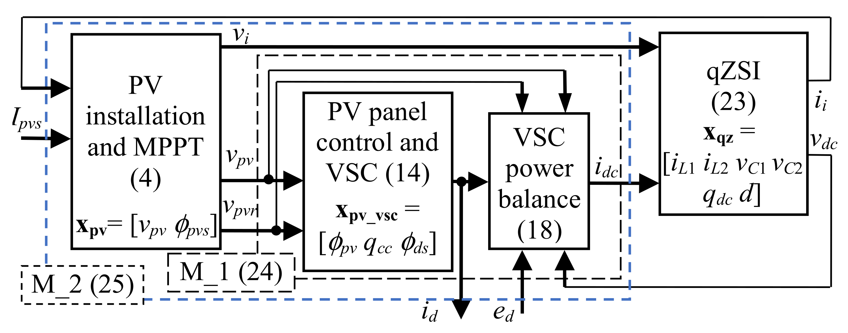
2.4. Model of the qZSI-PV System

The diagram of the qZSI-PV system with the small-signal models of all the components is presented in Figure 3, according to the previous sections. The SSA models (1) of the qZSI-PV system modules before obtaining the complete qZSI-PV system are shown in this subsection.

• Module #1 (M_1 in Figure 3): The PV panel control and grid-connected VSI (14), including the VSI power balance (18), are expressed as:

  $$\begin{array}{c}\frac{d}{dt}\left[\begin{array}{c}\mathrm{\Delta }{\varphi }_{pv}\\ \mathrm{\Delta }{q}_{cc}\\ \mathrm{\Delta }{\varphi }_{ds}\end{array}\right]=\underset{{\mathbf{A}}_{{\mathbf{M}}_{-}\mathbf{1}}}{\underbrace{\left[{\mathbf{A}}_{{\mathbf{p}\mathbf{v}}_{-}\mathrm{v}\mathrm{s}\mathrm{c}}\right]}}\left[\begin{array}{c}\mathrm{\Delta }{\varphi }_{pv}\\ \mathrm{\Delta }{q}_{cc}\\ \mathrm{\Delta }{\varphi }_{ds}\end{array}\right]+\underset{{\mathbf{B}}_{1\mathbf{M}\mathbf{-}\mathbf{1}}}{\underbrace{\left[\begin{array}{l}{\mathbf{B}}_{\mathbf{1}\mathbf{p}{\mathbf{v}}_{\mathbf{v}}\mathbf{v}\mathbf{s}\mathbf{c}}\hspace{1em}{\mathbf{0}}_{\mathbf{3}\mathbf{x}\mathbf{1}}\end{array}\right]}}\left[\begin{array}{c}\mathrm{\Delta }{v}_{pv}\\ \mathrm{\Delta }{v}_{pvr}\\ \mathrm{\Delta }{v}_{dc}\end{array}\right]\\ \left[\begin{array}{c}\mathrm{\Delta }{i}_{dc}\\ \mathrm{\Delta }{i}_d\end{array}\right]={\mathbf{C}}_{{\mathbf{M}}_{\mathbf{-}}\mathbf{1}}\left[\begin{array}{c}\mathrm{\Delta }{\varphi }_{pv}\\ \mathrm{\Delta }{q}_{cc}\\ \mathrm{\Delta }{\varphi }_{ds}\end{array}\right]+{\mathbf{E}}_{1{\mathbf{M}}_{\mathbf{-}}\mathbf{1}}\left[\begin{array}{c}\mathrm{\Delta }{v}_{pv}\\ \mathrm{\Delta }{v}_{pvr}\\ \mathrm{\Delta }{v}_{dc}\end{array}\right]+\underset{{\mathbf{E}}_{\mathbf{2}{\mathbf{M}}_{\mathbf{-}}\mathbf{1}}}{\underbrace{\left[\begin{array}{c}-G_{dcm}\\ 0\end{array}\right]}}\left[\mathrm{\Delta }{e}_d\right]\\ {\mathbf{C}}_{\mathbf{M}\mathbf{\_}\mathbf{1}}=\left[\begin{array}{c}\left(m_{d0}+G_{dcm}{k}_p^{cc}\right){\mathbf{C}}_{\mathbf{p}{\mathbf{v}}_{\mathbf{-}}\mathbf{v}\mathbf{s}\mathbf{c}}\\ {\mathbf{C}}_{\mathbf{p}{\mathbf{v}}_{\mathbf{-}}\mathbf{v}\mathbf{s}\mathbf{c}}\end{array}\right]-G_{dcm}\left[\begin{array}{ccc}{k}_p^{cc}{k}_i^{pv}& k_i^{cc}& 0\\ 0& 0& 0\end{array}\right]{\mathbf{E}}_{1\mathbf{M}\mathbf{-}\mathbf{1}}=\left[\begin{array}{ccc}-G_{dcm}{k}_p^{cc}{k}_p^{pv}& G_{dcm}{k}_p^{cc}{k}_p^{pv}& G_{dc}\\ 0& 0& 0\end{array}\right].\end{array}$$

  (24)
• Module #2 (M_2 in Figure 3): The PV installation (4) and the PV panel control, grid-connected VSI and VSI power balance (24) are represented by:

  $$\begin{array}{l}\frac{d}{dt}\left[\begin{array}{c}\Delta v_{pv}\\ \Delta {\varphi }_{pvs}\\ \Delta {\varphi }_{pv}\\ \Delta q_{cc}\\ \Delta {\varphi }_{ds}\end{array}\right]=\underset{A_{M\_2}}{\underbrace{\left[\begin{array}{cc}{A}_{pvm}& 0_{2x3}\\ B_{1M\_1}{H}_A& A_{M\_1}\end{array}\right]}}\left[\begin{array}{c}\Delta v_{pv}\\ \Delta {\varphi }_{pvs}\\ \Delta {\varphi }_{pv}\\ \Delta q_{cc}\\ \Delta {\varphi }_{ds}\end{array}\right]+\underset{B_{1M\_2}}{\underbrace{\left[\begin{array}{cc}{B}_{1pvm}& 0_{2x1}\\ B_{1M\_1}{H}_B{E}_{1pvm}& B_{1M\_1}{I}_{001}^{\mathrm{T}}\end{array}\right]}}\left[\begin{array}{c}\Delta i_i\\ \Delta v_{dc}\end{array}\right]+\underset{B_{2M\_2}}{\underbrace{\left[\begin{array}{cc}{B}_{2pvm}& 0_{2x1}\\ 0_{3x1}& 0_{3x1}\end{array}\right]}}\left[\begin{array}{c}\Delta I_{pv}\\ \Delta e_d\end{array}\right]\\ \left[\begin{array}{c}\Delta v_i\\ \Delta i_{dc}\end{array}\right]=\underset{C_{M\_2}}{\underbrace{\left[\begin{array}{cc}{I}_{10}{C}_{pvm}& 0_{1x3}\\ I_{10}{E}_{1M\_1}{H}_A& I_{10}{C}_{M\_1}\end{array}\right]}}\left[\begin{array}{c}\Delta v_{pv}\\ \Delta {\varphi }_{pvs}\\ \Delta {\varphi }_{pv}\\ \Delta q_{cc}\\ \Delta {\varphi }_{ds}\end{array}\right]+\underset{E_{1M\_2}}{\underbrace{\left[\begin{array}{cc}{I}_{10}{E}_{1pvm}& 0_{1x1}\\ I_{10}{E}_{1M\_1}{H}_B{E}_{1pvm}& I_{10}{E}_{1M\_1}{I}_{001}^{\mathrm{T}}\end{array}\right]}}\left[\begin{array}{c}\Delta i_i\\ \Delta v_{dc}\end{array}\right]+\underset{E_{2M\_2}}{\underbrace{\left[\begin{array}{cc}{0}_{1x1}& 0_{1x1}\\ 0_{1x1}& I_{10}{E}_{2M\_1}\end{array}\right]}}\left[\begin{array}{c}\Delta I_{pv}\\ \Delta e_d\end{array}\right],\end{array}$$

  (25)

  where

  $$\begin{array}{l}{H}_A=I_{100}^{\mathrm{T}}{I}_{10}+I_{010}^{\mathrm{T}}{I}_{01}{C}_{pvm}=\left[\begin{array}{cc}1& 0\\ 0& 0\\ 0& 0\end{array}\right]+\left[\begin{array}{cc}0& 0\\ 0& 1\\ 0& 0\end{array}\right]C_{pvm}\hspace{1em}\hspace{1em}{H}_B=I_{010}^{\mathrm{T}}{I}_{01}=\left[\begin{array}{cc}0& 0\\ 0& 1\\ 0& 0\end{array}\right]\\ I_{10}=\left[\begin{array}{cc}1& 0\end{array}\right]\hspace{1em}\hspace{1em}{I}_{01}=\left[\begin{array}{cc}0& 1\end{array}\right]\hspace{1em}\hspace{1em}{I}_{100}=\left[\begin{array}{ccc}0& 1& 0\end{array}\right]\hspace{1em}\hspace{1em}{I}_{010}=\left[\begin{array}{ccc}0& 1& 0\end{array}\right].\end{array}$$

  (26)

Finally, the SSA model of the qZSI-PV system is obtained from (23) and (25) as:

$$\begin{array}{l}\frac{d\Delta x_s}{dt}=A_s\Delta x_s+B_{2s}\Delta u_{s2}\Delta y_s=C_s\Delta x_s\\ A_s=\left[\begin{array}{cc}{A}_{s,11}& A_{s,12}\\ A_{s,21}& A_{s,22}\end{array}\right]B_{2s}=\left[\begin{array}{c}{B}_{1M\_2}\cdot T·E_{1qz}·E_{2M\_2}+B_{2M\_2}\\ B_{1qZ}\cdot (E_{1M\_2}·T·E_{1qz}+I_{2x2})·E_{2M\_2}\end{array}\right]C_s=\left[\begin{array}{ccc}{0}_{1x3}& \frac{1}{L_f}& 0_{1x6}\end{array}\right],\end{array}$$

(27)

where x_s = [Δv_pv Δϕ_pvs Δϕ_pv Δq_cc Δϕ_ds Δi_L1 Δi_L2 Δv_C1 Δv_C2 Δϕ_dc Δd]^T, u_2s = [ΔI_pv Δe_d]^T, y_s = [Δi_d] and I_2×2 is the 2 × 2 identity matrix.

Unlike the Simulink and PSCAD models in [25], the SSA model in (27) can be custom programmed to create a software tool for studying qZSI-PV system dynamics in time and Laplace domains. This is a relevant contribution in assessing qZSI-PV system dynamic behavior.

2.5. Validation of the qZSI-PV System Model

The SSA model (27) of the qZSI-PV system shown in Figure 1 involving the data shown in

Table 1. The qZSI-based PV power system parameters.

Circuit and Control	Parameters	Data
PV array	Np × Ns	55 × 42
	G, T	500 W/m2, 25 °C
PV installation	Rc, Cp	0.0667 Ω, 10 mF
qZSI source network	L1 = L2, r1 = r2	0.3 mH, 0.011 Ω
	C1 = C2, R1 = R2	3 mF, 0.006 Ω
	fsw	10 kHz
VSI	Rf, Lf, Cf	≈0 Ω, 0.4 mH, 100 ĉF
MPPT control	$k_p^m, k_i^m$	0.01 Ω, 0.5 Ω/s
PV control	$k_p^{\mathit{pv}}, k_i^{\mathit{pv}}$	1.8 Ω−1, 75 Ω−1/s
CC control	$k_p^{\mathit{cc}}, k_i^{\mathrm{cc}}$	0.424 Ω−1, 150 Ω−1/s
D control	$V_{\mathit{dc},p}^{*}$	800 V
	$k_p^{\mathit{dc}}, k_i^{\mathit{dc}}$	0.016 V−1, 125 V−1/s
	$k_p^L$	10−4 A−1

is validated in Figure 4. The PV panel delivers 1 kV 140 kW to a DC power system connected to an ideal 0.4 kV AC network. In the validation, the PV panel has a 55 × 42 60 W PV Solarex MSX60 module [2] with an irradiance level of G = 500 W/m² and a temperature T = 25 °C, while the qZSI works with a duty cycle D = 0.06.

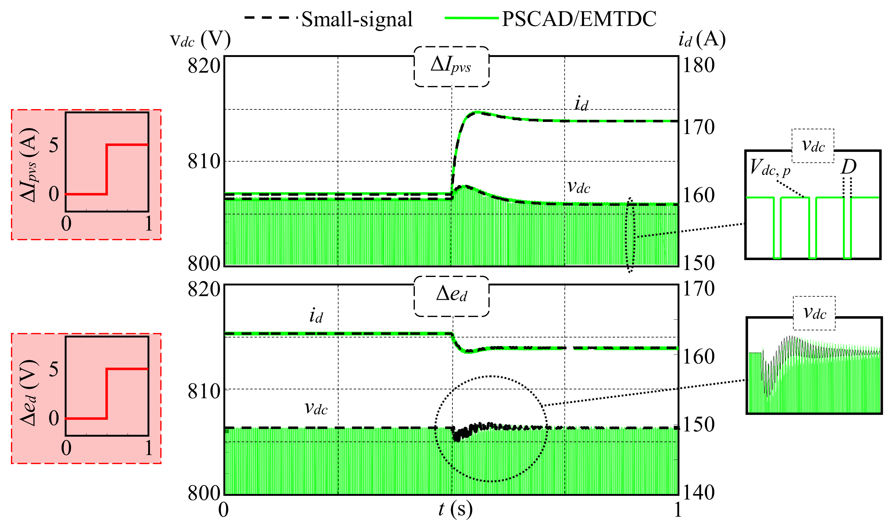
The transient performance of the DC peak voltage v_dc and the grid d-current i_d is studied when a small perturbation of 5 A and 5 V around the operating point values of the PV panel current I_pvs (94 A) and the grid d-voltage e_d (400 V) is introduced (see red plots in Figure 4). 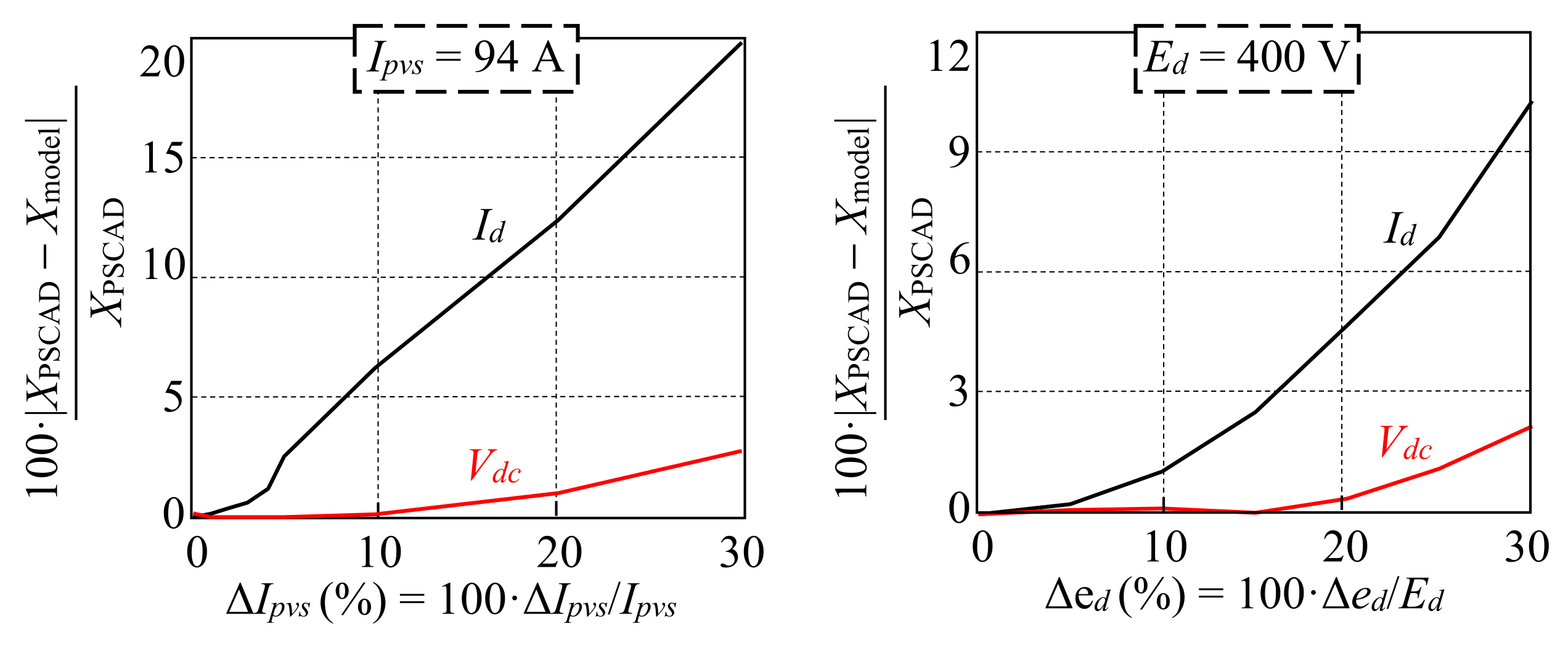The fair accuracy of the qZSI-PV system model is validated by comparing its dynamic response to PSCAD/EMTDC simulations obtained with the circuit in Figure 1. It must be noted that the qZSI-PV system model must be validated with a small perturbation around the operating point because it is a small-signal model that cannot reproduce the dynamics related to significant changes in the the qZSI-PV system operating point. In order to illustrate the previous comment, Figure 5 shows the stationary deviations (differences between PSCAD/EMTDC and the small-signal model results) of the DC peak voltage v_dc and the grid d-current i_d for different perturbations of I_pvs and e_d. It can be observed that the validity of the model highly depends on the variables of the model (e.g., an I_pvs perturbation of 20% leads to a non-acceptable error of 12% in the stationary value of the grid d-current). In general, the accuracy of the small-signal model is fair for perturbations smaller than 10%.

3. Examples

Stability problems in the qZSI-PV system shown in Figure 1 are analyzed with the data shown in Table 1 and using the proposed SSA model. Solutions to mitigate instabilities are also discussed. The PV panel delivers 1 kV 140 kW to a DC power system connected to an ideal 0.4 kV AC grid. Note that an ideal AC grid is considered in this study because we only analyze the qZSI-PV system dynamics and not the interaction between the qZSI-PV system and the grid. In such conditions, the VSI filter capacitor C_f does not affect the obtained results. If the dynamic interaction between the qZSI-PV system and the grid were to be studied, a weak AC grid should be considered. In this case, the capacitor Cf affects the system behavior. The usual range of 1–1.5 kV DC for large-scale PV power systems (P_pv > 10 kW) is considered in the application. This voltage level reduces the initial investment and total cabling required [6,19,24]. In the application, the PV panel is based on PV Solarex MSX60 modules and configured with 42 modules connected in series and 55 arrays connected in parallel. The module manufacturer data give the following information: V_oc = 21.0 V, I_sc = 3.7 A, V_max = 17.2 V, I_max = 3.6 A, P_max = 60.0 W at G = 1000 W/m² [2]. The voltage and current MPP values corresponding to G = 500 W/m² are V_mpp = 16.7 V and I_mpp = 1.8 A. These MPP values yield a PV panel voltage V_pv = 702.9 V, PV panel current I_pvs = 97.35 A and a power P_pv = 68.2 kW. The analyzed cases are based on these values. It is also worth noting that the IGBT switching frequency f_sw is set to 10 kHz as in [6,15,17].

The system stability is investigated using the SSA model of the qZSI-PV system in Section 2 and PSCAD and PSIM simulations in the following three cases:

• Case #1 (reference case): This is the stable operating point at steady state with N_p = 55, N_s = 42, G = 500 W/m² and T = 25 °C (V_mpp = 702.9 V, I_mpp = 97.7 A; see left of Figure 2a);
• Case #2: The influence of the irradiation level G on PV system stability is studied. The stability of the steady-state operating point in case #1 when the irradiation level increases to G = 800 W/m² (V_mpp = 712.3 V, I_mpp = 156.4 A; see right of Figure 2a) is analyzed;
• Case #3: The impact of the total number of PV arrays connected in parallel N_p on the PV system stability is studied. The stability of the steady-state operating point in case #1 when N_p increases to N_p = 100 (V_mpp = 702.9 V, I_mpp = 177.8 A; see left of Figure 2a) is analyzed.

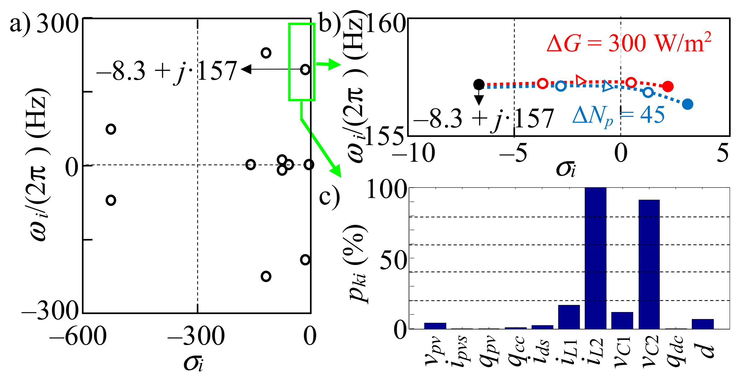
Case #1’s eigenvalues λ_i = σ_i + j·ω_i are derived from the SSA model of the qZSI-PV system, while the terms σ_i and ω_i/(2π) are shown in Figure 6. These eigenvalues verify the system stability because they are not in the right half-plane (RHP). Figure 6b shows the trajectories of the eigenvalues related to the unstable mode if the irradiance level G (case #2) or the number of PV panels in parallel (case #3) is varied. It is worth noting that as pointed out in Section 2.3.1, a higher irradiance level or number of PV arrays connected in parallel causes system instability because the eigenvalue of the oscillatory frequency f_i = ω_i/(2π) = 157 Hz moves into the RHP. This is illustrated in the PSCAD and PSIM time domain simulations of Figure 7, whereby the increase of G from 500 W/m² to 750 W/m² causes system instability. This increase carries from one PV power system operating point to another and the parameters of the PV power system model are updated accordingly. As an example, the resistance R_pv value of the PV installation small-signal equivalent circuit in Figure 2c is labelled in Figure 7 for the two irradiance levels. As the simulation programs used in the study do not include any PV panel model, the PV panel small-signal circuit derived from the linearization of the I-V plots near the PV panel MPP, shown in (3) and Figure 2c, is applied. According to this, the resistance R_pv value of the PV panel small-signal equivalent circuit in (4) is updated from the MPP values. These values are obtained from the I-V plot of a PV panel [4,25] and the MPPT control depending on the value of the PV panel variables (i.e., N_p, N_s, G and T in Figure 2a). The PV panel tries to supply the rated power of the PV power system after the irradiance level steps up but the PV power system becomes unstable, while the frequency of unstable oscillations measured in the PSCAD and PSIM simulations (i.e., ≈150 Hz) approximately matches the oscillatory frequency of the eigenvalue. Note that although the time domain simulation of PSCAD and PSIM is not exactly the same, both simulations verify the previous results. The same is true for higher numbers of PV arrays connected in parallel, which are not shown here for the sake of time.

In order to obtain solutions to improve the qZSI-PV system stability, the PFs of each state-space variable k (see Figure 3) on each mode i are calculated as p_ki = φ_ki·ψ_ik, with φ_ki and ψ_ik being the components of the right and left eigenvectors, respectively. According to this, Figure 6c shows the PFs of the eigenvalue related to the unstable mode. 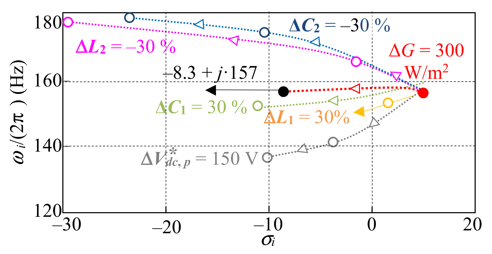The results indicate that the qZSI inductors (L₁ and L₂) and capacitors (C₁ and C₂) have the largest PFs for the unstable mode, suggesting that qZSI-PV system stability could be improved by modifying the above qZSI parameters. This possibility is verified with the trajectories of the eigenvalue related to the unstable mode when the qZSI-PV system is operating under case #2 conditions and the inductors and capacitors are varied (see Figure 8). It is noted that lower L₂ and C₂ and higher L₁ and C₁ lead to system stability because the eigenvalue moves out of the RHP.

In light of the above, qZSI-PV system stability should be considered in qZSI inductor and capacitor design; however, as these values are usually compromised by qZSI performance [6], it is interesting to look for other approaches to improve the qZSI-PV system stability by means of control or external variables. According to Section 2.3.1, the increase of the steady-state qZSI output voltage V_dc reduces the virtual conductance G_dc (18), improving the qZSI-PV system stability; thus, the peak voltage reference $V_{dc,p}^{*}$ seems to be a suitable candidate that can be used as an external variable to upgrade the qZSI-PV system stability. This solution is validated with the trajectory of the eigenvalue related to the unstable mode when the qZSI-PV system is operating under case #2 conditions and the DC peak voltage reference $V_{dc,p}^{*}$ increases from 800 to 950 V (see Figure 7b). This allows system stability to be obtained because the eigenvalue moves out of the RHP, although increasing the qZSI output voltage V_dc could lead to higher switch stress and a lower voltage utilization ratio.

The stability studies show that:

• The impacts of qZSI inductors and capacitors on qZSI dynamic behavior [8] are extended to qZSI-PV system transient performance;
• The qZSI-PV system operating points, particularly the active power P delivered to the AC grid and the steady-state qZSI output voltage V_dc, have an impact on instability. The study of the duty cycle in [21,22] is related to the previous impacts of voltage V_dc.

The PSCAD and PSIM simulations in Figure 7 verify the above conclusions. The decrease of L₂ from 0.3 mH to 0.24 mH (ΔL₂ = −20%) and the increase of $V_{dc,p}^{*}$ from 800 V to 950 V ($\mathrm{\Delta }{V}_{dc,p}^{*}$= 150 V) return the qZSI-PV system to stability after becoming unstable due to the growth in the irradiance level. Although not shown for the sake of space, the same is true for the above parameters.

4. Conclusions

The first part of the paper presents the SSA model of the qZSI-PV system in order to study the stability, considering all the main components and controls. This model allows the system stability to be analyzed via the system eigenvalues, PFs and time domain simulations. The accuracy of the proposed small-signal model is validated from PSCAD/EMTDC simulations. Acceptable results are obtained for perturbations smaller than 10%. The second part of the paper (Section 3) contributes the application of the proposed model to the qZSI-PV system stability assessment and studies the system parameter variation impacts on stability. The following conclusions are drawn:

• The most important factor associated with system stability is the operating point;
• The increase in the active power delivered to the AC grid can cause system instability;
• System stability is also affected by the DC peak voltage; that is, high DC peak voltage reference values reduce the impacts of the increase in the active power delivered to the AC grid but lead to high switch stress and low voltage utilization ratios;
• The qZSI component design (low values of L₂, C₂ and high values of L₁, C₁) is crucial in improving system stability.

The above contributions are validated using PSCAD time-domain simulations. The following further studies could be conducted using the model presented in this paper: (i) simplification of the proposed SSA model to analytically characterize the obtained conclusions; (ii) development and use of a frequency-based model for stability assessment of grid-connected PV power systems; (iii) study of the dynamic interactions between the qZSI-PV system, VSI filter capacitor and grid.