Demonstration Study of Voltage Control of DC Grid Using Energy Management System Based DC Applications

Abstract

This paper is about the development of the real-time direct current (DC) network analysis applications for the operation of DC power systems. The applications are located in the central energy management system (EMS) and provide the operator with the optimal solution for operation in real time. Developed DC applications are not limited by voltage level. Applications can be used at all DC voltage levels such as low voltage, medium voltage and high voltage. A program configuration and sequence for analyzing the DC distribution system are suggested. Algorithms of each program are presented and the differences when compared with the processes of the applications of the existing alternating current (AC) systems are analyzed. The DC grid demonstration site at the Korea Electric Power Corporation (KEPCO) power testing center is introduced. The details of EMS and applications installation are described. The developed DC applications were installed in the EMS of the demonstration site and verification tests have been carried out. The configuration of the test scenario for testing the voltage control of the DC network is described. The voltage control result is analyzed and the measured data and the results of the applications are verified for compatibility by comparing them with the results of an off-line simulation tool. Finally, the future direction of the development of technology for the operation of the DC grid is introduced.

1. Introduction

Direct current (DC) power system technology attracts attention as an interconnection solution for increasing DC-based distributed energy resources such as energy storage systems (ESS), photovoltaic systems (PV) and large DC consumers such as internet data centers. As the power conversion technology utilizing power semiconductors advances, conversion from AC to DC, stepping up/down of DC voltage have become possible and are now available for application in power system in various ways. Accordingly, research studies are underway globally on the design and operation of ways to reduce the losses occurring in the process of converting DC to AC by directly connecting DC sources to DC loads and to increase the capacity and distance of the power transmission. [1,2,3,4]

At the Korea Electric Power Corporation (KEPCO) Research Institute, teams are doing research for the commercialization of things ranging from core equipment to protection and operation technology for DC distribution, they have established a demonstration site and are carrying out operation tests. They have established real DC distribution lines for supplying long distance low load electric power in Gwangju that is currently in operation [5]. At the Gochang power testing center of KEPCO, a 6 km DC distribution demonstration site has been established and the necessary infrastructure for testing DC distribution equipment and operation technology is now available. Recently, a DC island which connects the renewable generators and loads in Seogeochado Island in Jindo County with 5 km DC lines was completed [6].

As the number of distributed energy resources and loads interconnected to the DC distribution network increases, the configuration of the distribution network is getting more complicated from the unidirectional radial lines to the mesh network. In such a mesh type DC grid, it is difficult to ensure stability only with the constant voltage operation of the reference converter. A solution is needed which informs the operator of the control that needs to be activated in case of a violation like an overvoltage in the system, so the importance of the energy management system (EMS) for the operation of the DC distribution network has grown.

In power transmission systems, many applications are installed and run in the EMS for the operation of large-scale networks and as distributed energy resources also increase in power distribution systems, research studies to secure the systems and applications to handle situations have been conducted. The DC power system is very different in the operation characteristics of the equipment and system parameters from the AC power system. Therefore, we need EMS and applications dedicated to and capable of analyzing the DC power system considering the characteristics of the DC power system and providing solutions for its operation. This paper describes items related to the development of the applications which are installed in the EMS for the operation of the DC distribution network or DC microgrid and can analyze the DC power system in real-time. The configuration and algorithm of DC power system analysis applications are suggested, and issues regarding the establishment of the DC distribution network are handled. Finally, details of the demonstration tests and results are presented and analyzed.

2. DC Power System Analysis Applications

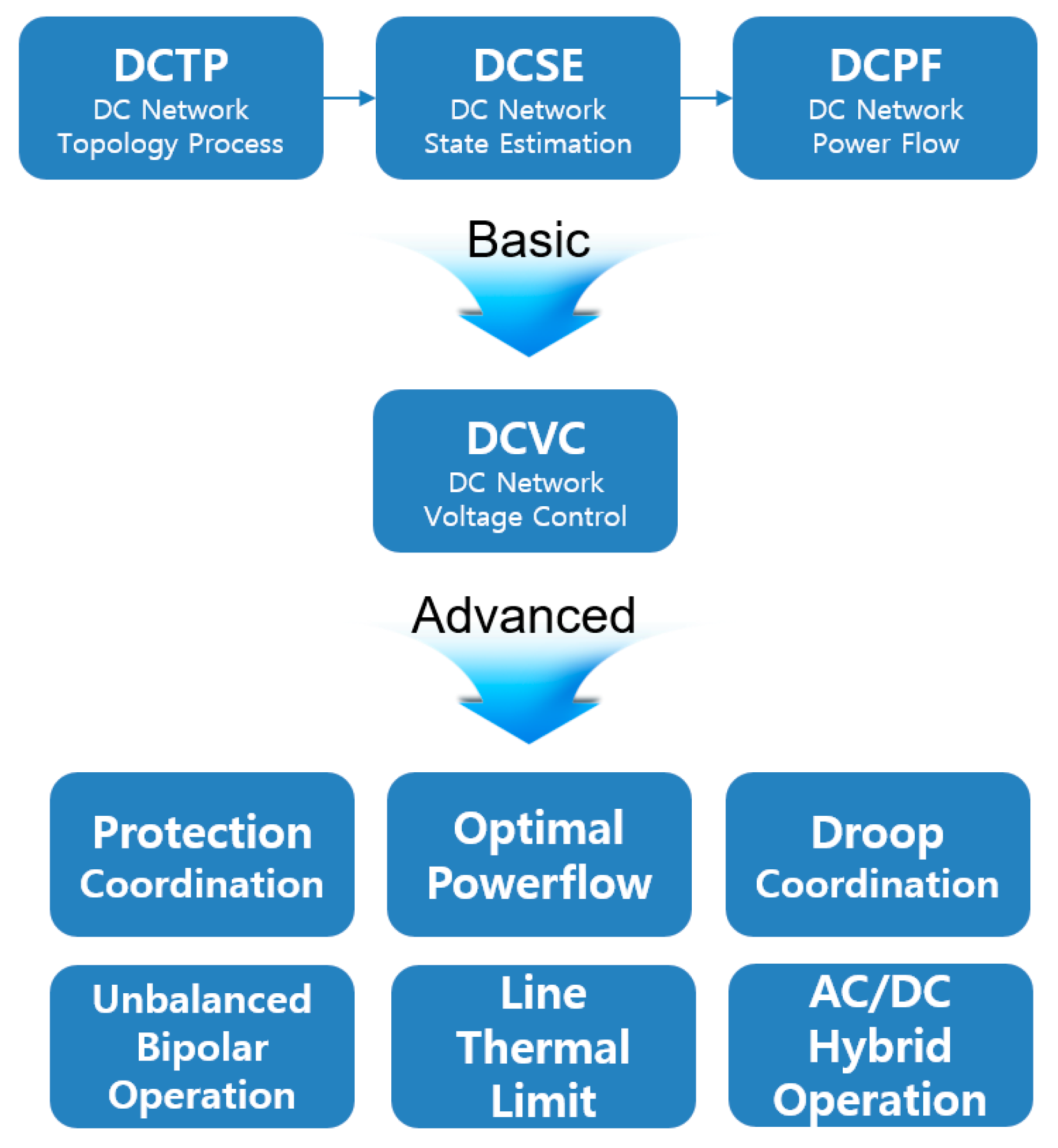
2.1. Program Configuration and Sequence

The typical network analysis applications used in the EMS for AC power systems are listed below [7,8,9,10,11,12,13,14]:

• Topology process (TP)
• State estimation (SE)
• Power flow (PF)
• Contingency analysis (CA)
• Short circuit analysis (SCA)
• Optimal power flow (OPF)

There are many EMS applications other than those mentioned above used in power system analysis. Especially in the case of transmission EMS for the operation of large-scale AC power systems, various applications for analyzing the stability of power systems have been developed and used and sometimes verified commercial applications from outside are used in connection with EMS in real-time. Recent research studies are focused on enhancing the stability of the distribution system by developing applications for power system analysis of distribution networks or microgrids.

The most essential ones among the program of network analysis are topology process and state estimation. These two programs shall be executed first for other power system analysis applications to run and the compatibility shall be ensured for the results of other applications to be reliable.

The topology process is the program generating the bus information by checking the connectivity of equipment and open/closed status of breakers by grouping the nodes [15,16]. There are nodes at both ends of all equipment such as circuit breakers, lines, etc. Equipment links are traced in the database based on nodes and bus numbers are given to the segments by nodes with the same voltage, and this process is called node-bus mapping. Figure 1 shows the topology process concept.

In Figure 1, on the left is a real system model and on the right is a mathematical model for power system analysis. This is the process in which bus and connection information, both of which are the input parameters for all power system analysis algorithms are determined and it is the power system analysis program that is executed first. This program uses the measurement data as input and it carries out various pre-processing operations such as topology error analysis.

Measured data include some errors because of various field situations such as the error of communication equipment and synchronization problems, therefore it is difficult to use the measured data as input to power system analysis without some processing. The program that generates the input data for power system analysis correcting such errors is the state estimation.

Figure 2 shows the conceptual diagrams for indicating the necessity for state estimation. If the graphs in Figure 2 are for power flow equations, all measured data shall be on the line of one power flow equation in ideal cases. However, in reality, the measured data includes some errors. Thus, it is impossible to derive a power flow equation that satisfies all measured data, so SE derives the power flow equation which minimizes errors and calculates the new SE data which exist on the line for that equation. The least squares method is used to minimize these errors. All the programs run after state estimation use the results of state estimation as input, not the measured data.

Topology process and state estimation are fundamental processes for power system analysis in applications executed in real-time. Applications executed thereafter are selectively installed and used according to the strategy of power system operation. As mentioned above, although the reference converter of the slack bus takes the role of balancing supply with demand in a DC power system, there may be regional voltage violation phenomena due to overload or overinjection. In the case of voltage violation, there are two ways to clear it. One is to adjust the output voltage of the reference converter, the other is to adjust the active power output of the distributed energy resources. In the power system with a variety of distributed energy resources and complicated mesh network structure, it is essential to have a voltage control program that provides an accurate solution that can clear the voltage violation in real-time.

In this study, three kinds of pre-processing applications (DC topology process, DC state estimation, DC power flow) and one DC voltage control application have been used for the DC power system analysis and these are named as indicated below.

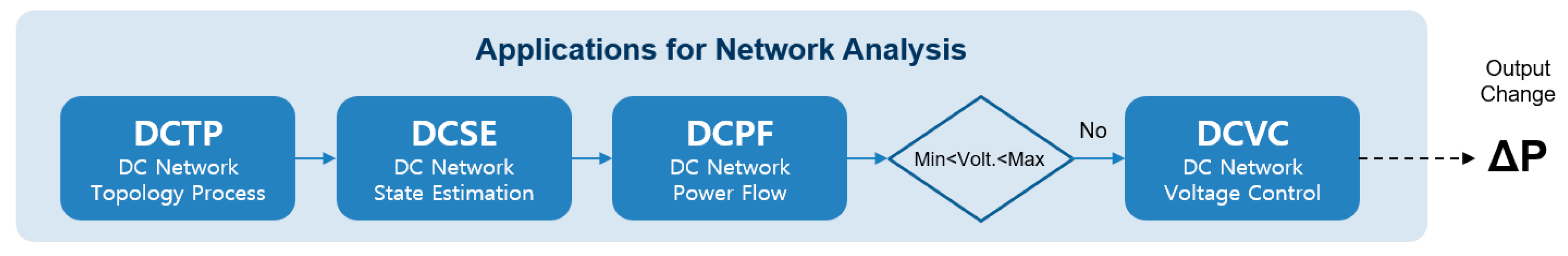
• DC network topology process (DCTP)
• DC network state estimation (DCSE)
• DC network power flow (DCPF)
• DC network voltage control (DCVC)

Figure 3 shows the operation sequence of four programs. DCTP, DCSE and DCPF are pre-processing applications and they process the measurement data so that DC power system analysis can be done. Thereafter, if a voltage violation occurs, the DCVC application provides the operator with the solution to control the voltage.

2.2. DC Power System Analysis Algorithm

Table 1. Analysis parameters of DC and AC networks.

Category	AC Network	DC Network
Variable	Frequency, Voltage, Current, Angle	Voltage, Current
Line parameter	Resistance, Inductance, Capacitance	resistance
Network topology	A, B, C, Neutral	(+), (−), N
Power balancing	Frequency	Voltage
Demand response	Constant voltage constant frequency (or Droop control)	Constant voltage (or Droop control)
grounding	Multi-grounding	Isolated terra
Voltage level	Transformer ►Integrated matrix (Per Unit method)	DC/DC converter ►Seperated matrix
Voltage control	Capacitor, Over load tap changer, Under load tap changer	Reference voltage control, Power output control
Approved voltage	Transmission system: ±5% distribution system: ±10%	±10% (Converter approved voltage)
Algorithm	Main algorithm of state estimation and power flow

shows the difference between AC and DC power systems from the viewpoint of power system analysis.

There is no frequency and reactive power in DC power systems. Also, instead of transformers, there are DC/DC converters in DC power systems which makes it difficult to handle the impedance, unlike the case of AC transformers, so while power systems with different voltage levels can be analyzed using one matrix with a per unit system in AC power systems, different voltage levels shall be analyzed using a separate matrix in DC power systems. That is, power systems with different voltage levels shall be considered as separate islands and they must be analyzed separately too.

Basic algorithms of individual processes such as state estimation and power flow for AC power systems are introduced in many books and articles. In this paper, things to be considered for applying such processes to DC power systems and any differences in formulas are mainly described.

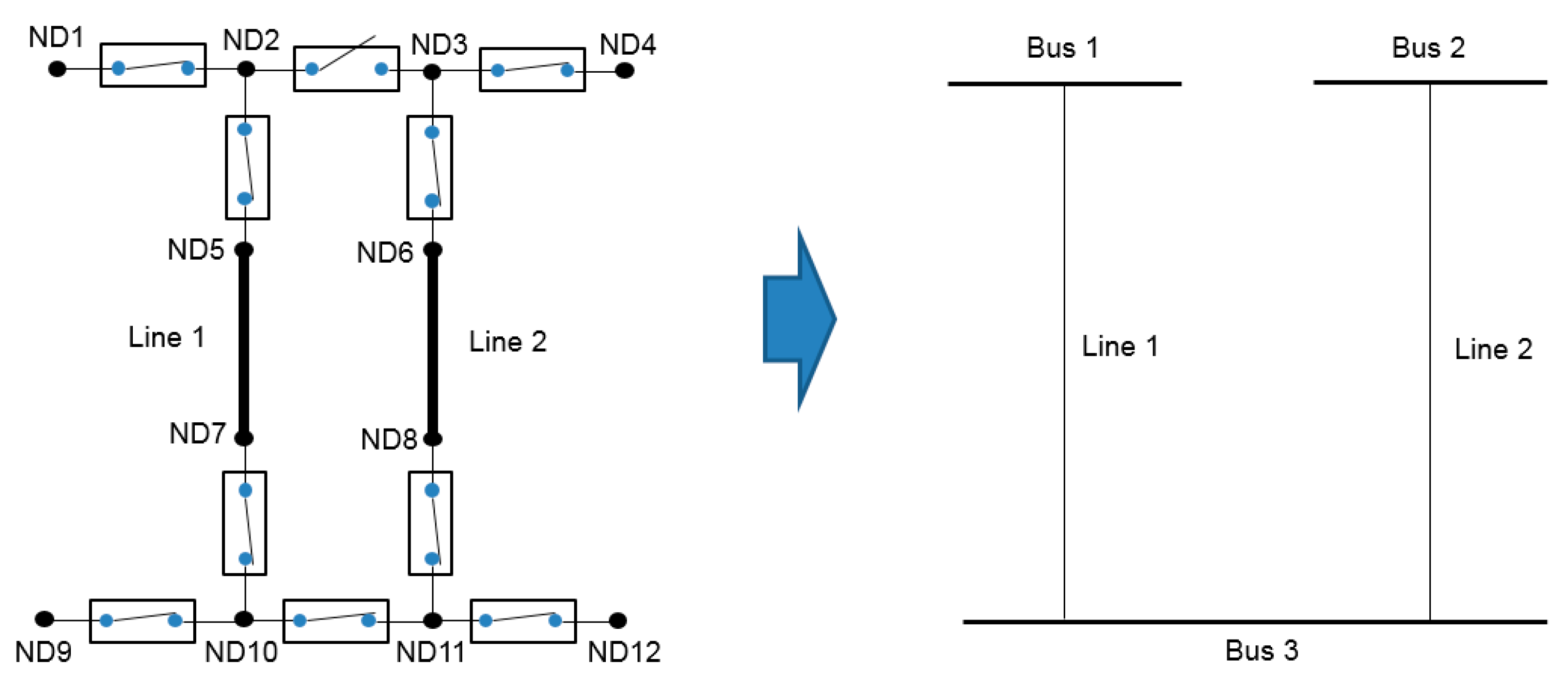
2.2.1. DC Network Topology Process (DCTP)

The topology process for DC power systems is not much different from that of AC power systems. However, the devices listed below which don’t exist in AC power systems need to be specifically taken care of in the database and programs:

• Converters for interconnecting with distributed energy resources → handled as sources and loads
• DC/DC converters → power systems at both ends are considered as islands
• Bipolar DC network → database with +/− pole structure is applied

As shown above, regarding converters, processing them as loads or sources, processing connected power systems as islands are important in DC power systems. Described below is the process for State Estimation of DC power systems.

• (Step 1) Select one bus.
• (Step 2) Bus grouping is executed using information on lines connected to the bus.
• (Step 3) Check if all buses have been grouped.
• (Step 4) If the condition in (Step 3) has been satisfied, the process moves to (Step 5) and unless, retry (Step 1) to (Step 2).
• (Step 5) Check whether there are conditions like the followings in the group.
  • At least two buses exist.
  • Bus voltages are available among the measured data.
  • Check whether there are at least one generator and load, or there are two or more AC/DC converters.
• (Step 6) If (Step 5) is satisfied, island numbers are given to the corresponding group.
• (Step 7) Equipment belonging to the island without numbers in (Step 6) is set to be stopped.

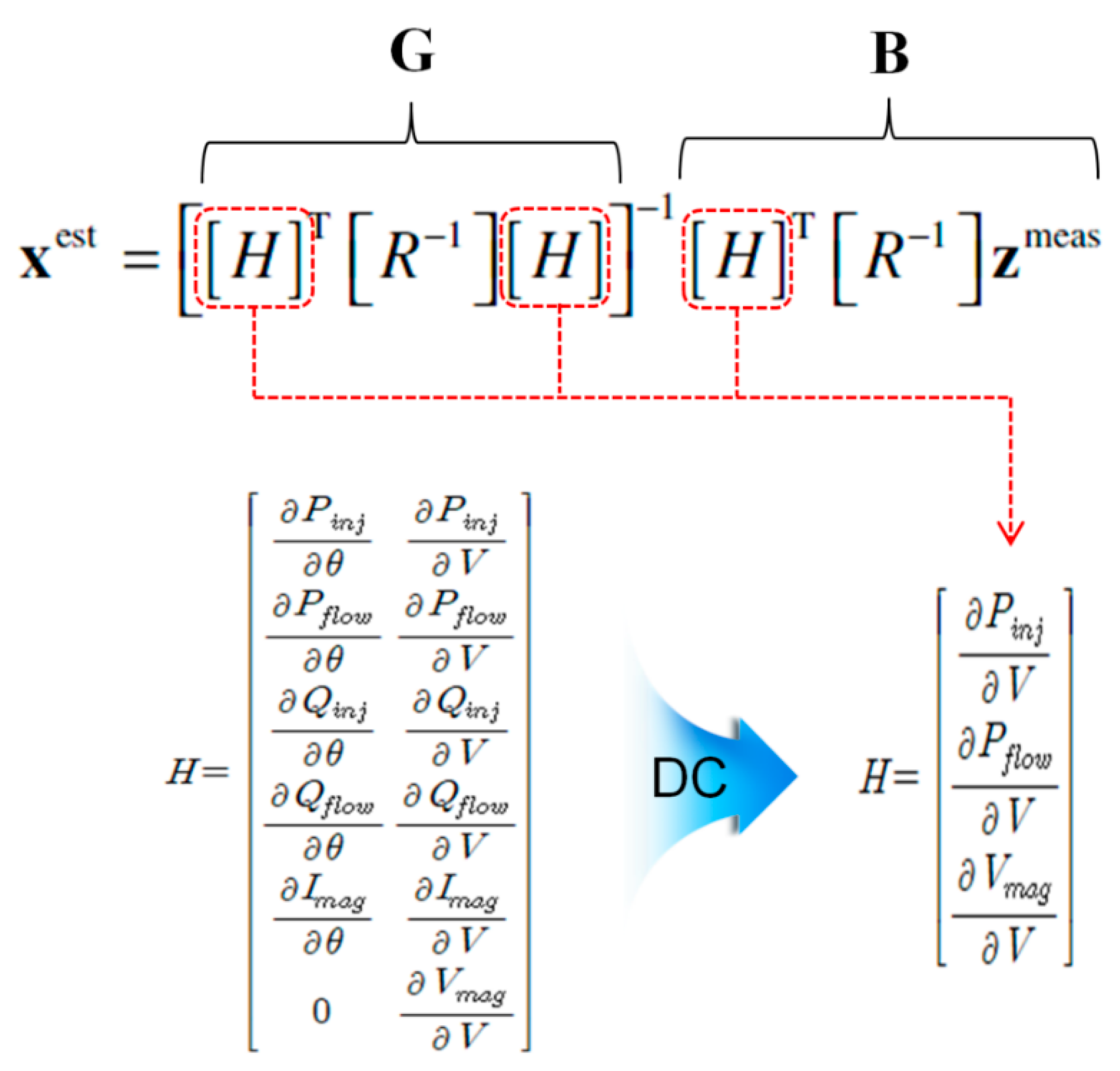
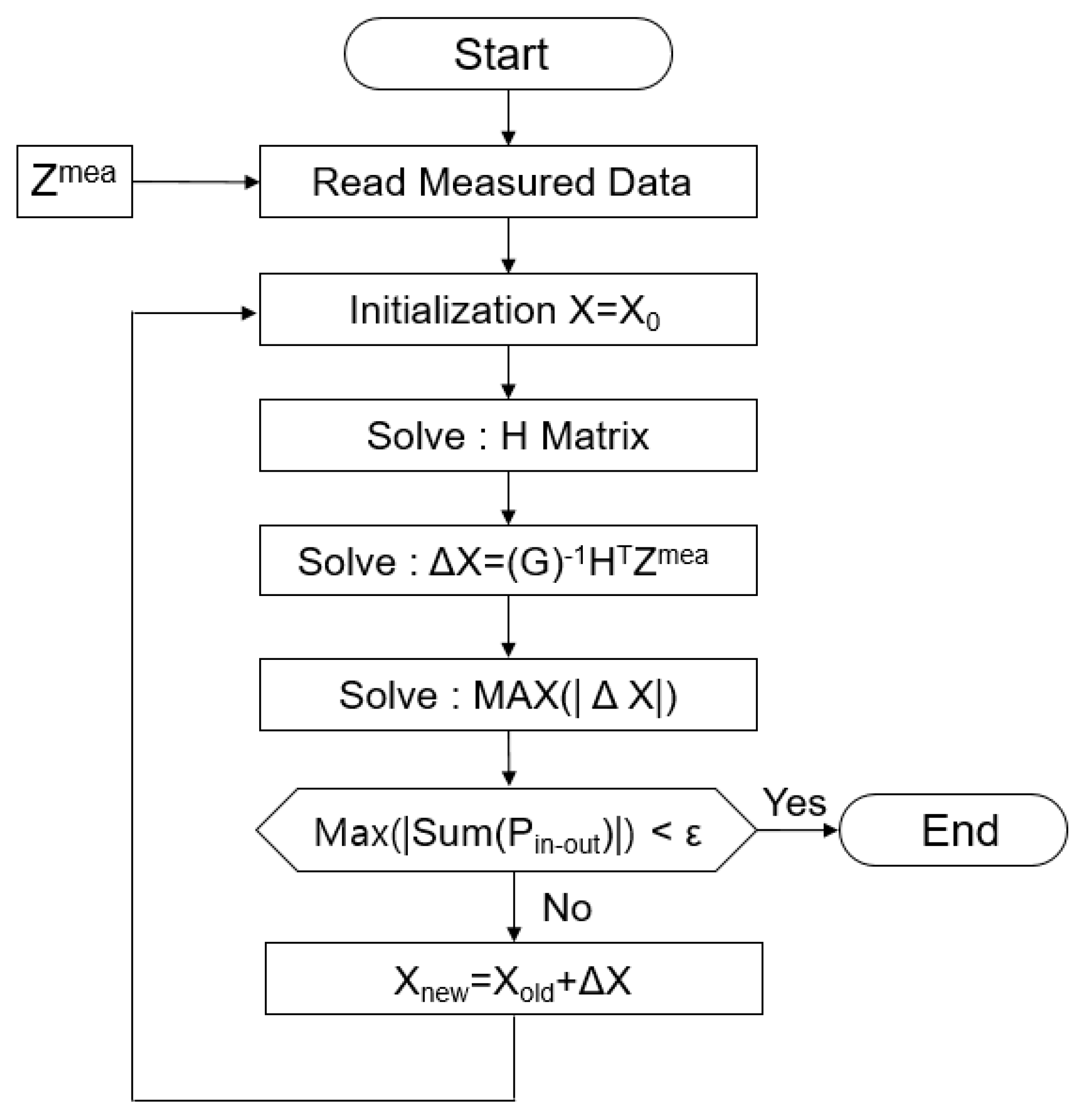
2.2.2. DC Network State Estimation (DCSE)

The basic process of State Estimation in DC network is similar to that of AC power systems [17,18,19,20,21,22,23,24,25,26,27]. The conventional equation of state estimation is as follows:

[Z_meas] = [H([X])] + [e]

(1)

where Z_meas: measurement data (bus injections, line flows, bus angles, bus voltages), H(X): true system state (power flow equations), X: state variables (bus angles, bus voltages) and e: measurement errors:

Min ∑{W_i·(Z^meas − H(X))²}

(2)

where W_i: weighted factor

The purpose of state estimation is to minimize the error in Equation (1). Equation (2) shows the objective function and the following is the final equation to solve the optimization problem:

X_est = [[H]^T·[R⁻¹]·[H] ]⁻¹·[H]^T·[R⁻¹]·Z_meas

(3)

where X_est: estimated variables (bus angles, bus voltages) and R: matrix of weighted factors.

For a DC grid, the matrix shall be configured using DC power system parameters instead of those of an AC power system. Figure 4 shows the difference between the state estimation matrix equations of AC power systems and those of DC power systems.

X_est = (V_est¹, V_est², V_est³ … V_estⁿ)

(4)

where V_n: voltage at bus-n

Z_meas = (P_meas¹, P_meas², … P_measⁿ, F_meas^i−k, …, V_meas1, V_meas², …, V_measⁿ)

(5)

where P_measⁿ: sum of measured active power injection on bus n, F_meas^i−k: measured active power flow of line between bus i and bus k and V_measⁿ: measured voltage on bus n.

Figure 5 shows the flowchart of DC network state estimation.

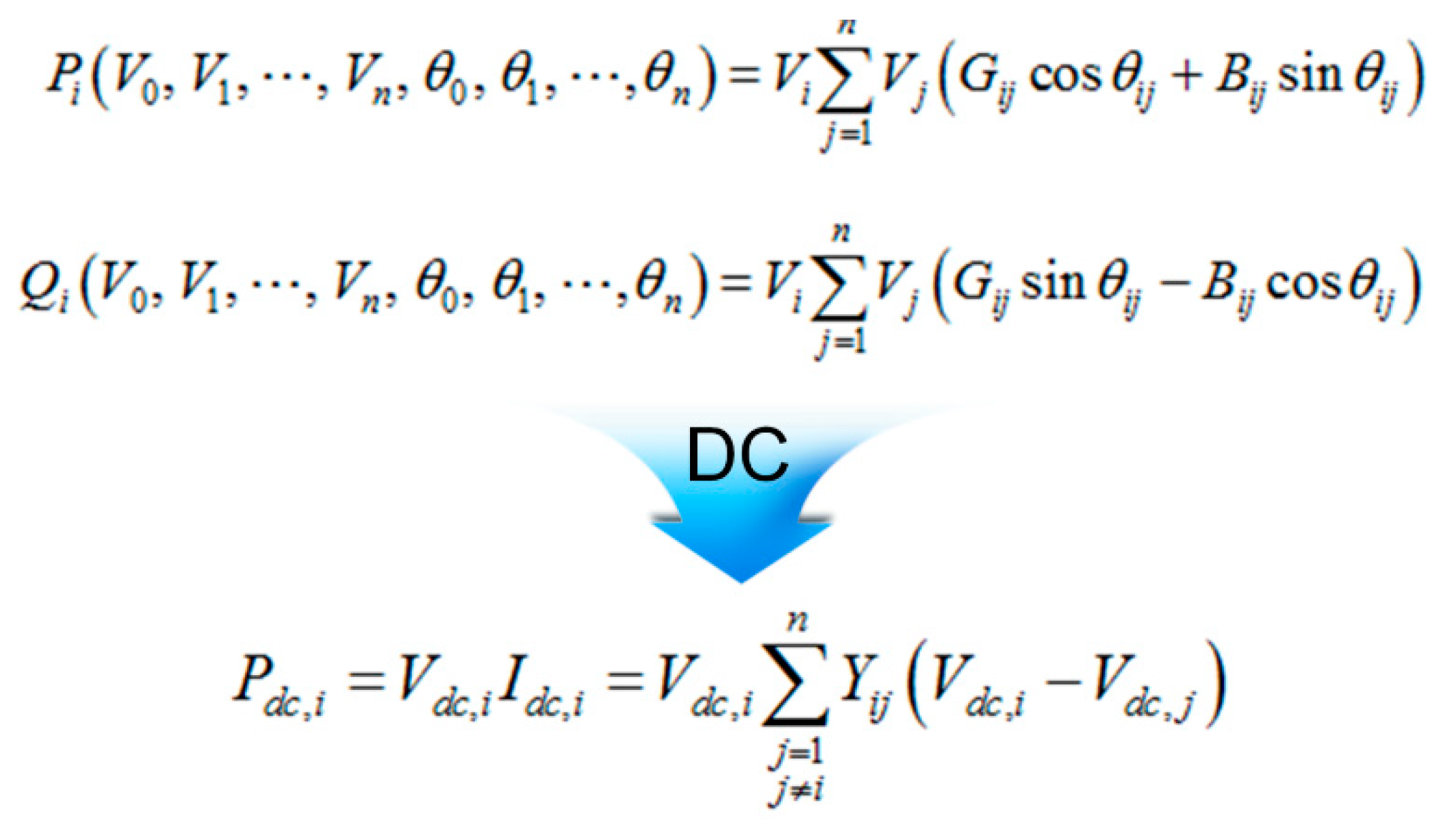
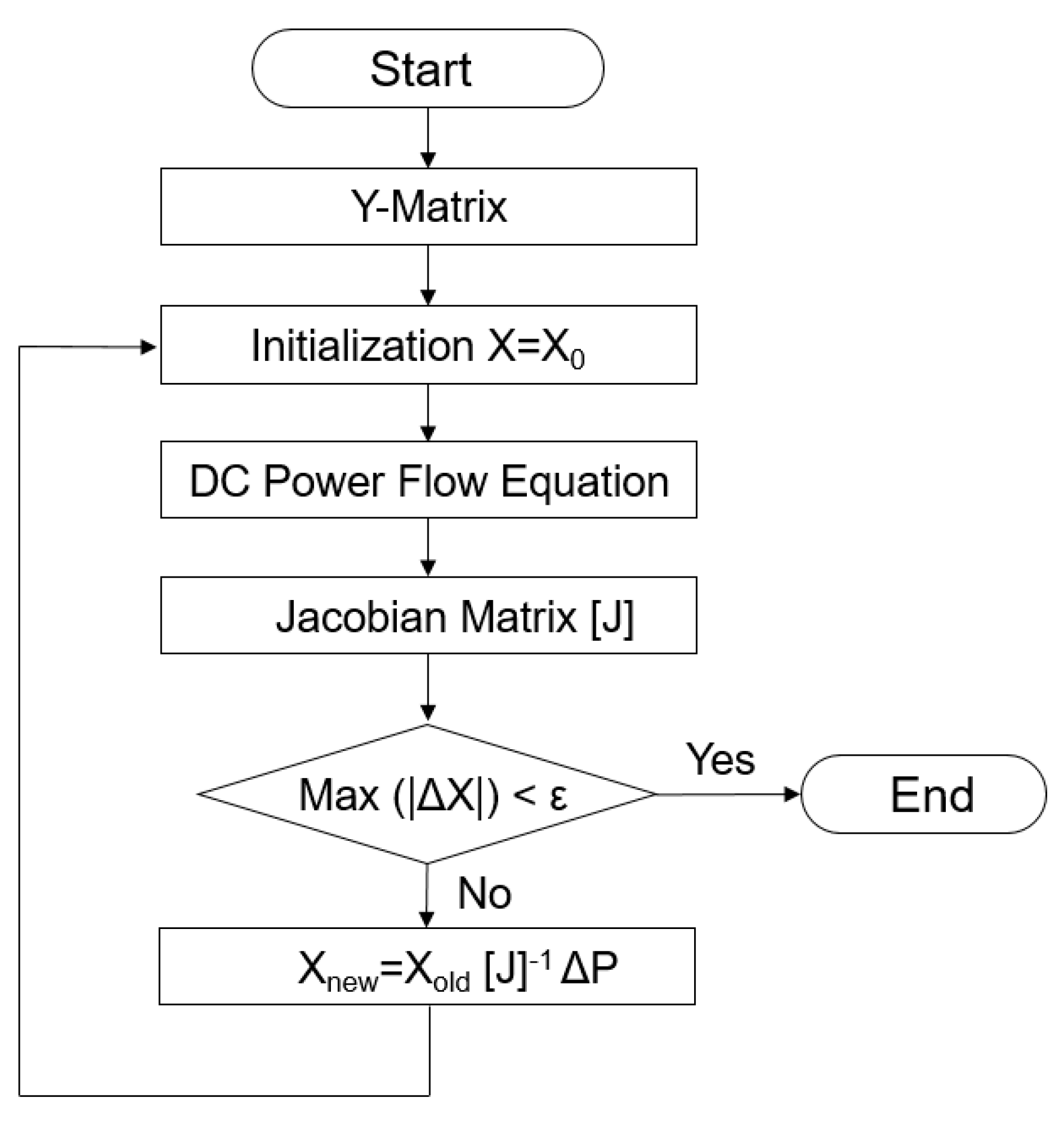
2.2.3. DC Network Power Flow (DCPF)

Although flow calculation algorithm is similar to that of an AC power system, DC power flow equations must be used for calculations. Figure 6 shows the difference between the power flow equations of AC and DC power systems [28,29,30].

Figure 7 shows the flowchart of the power flow calculation for DC power systems.

State estimation is to obtain the solution of the optimization function for clearing the mismatch of the injection power to the bus, and power flow calculation is to obtain the solution that satisfies the power flow equation. There are many differences between the two programs, from the purpose and structure of the matrix to the criteria for convergence.

Table 2. Difference between DC power flow and DC state estimation.

Category	State Estimation	Power Flow
Variable	All Measured Data (Voltage, Power)	V (Generator/Load Bus), P (Slack Bus)
Input	All Measured Data (Voltage, Power)	P (Generator/Load Bus), V (Slack Bus)
Equation	X=[HTR−1H]−1·[HT][R−1]Zmeas	X = J−1 B
Control	Bad Data Process	V (Generator/Load Bus), P (Slack Bus)
Convergence	Threshold > Pmismatch	Threshold > ΔX
Mismatch	Bus In/Out Mismatch Exist	No Mismatch

shows the difference between the two applications, state estimation and power flow of DC power systems.

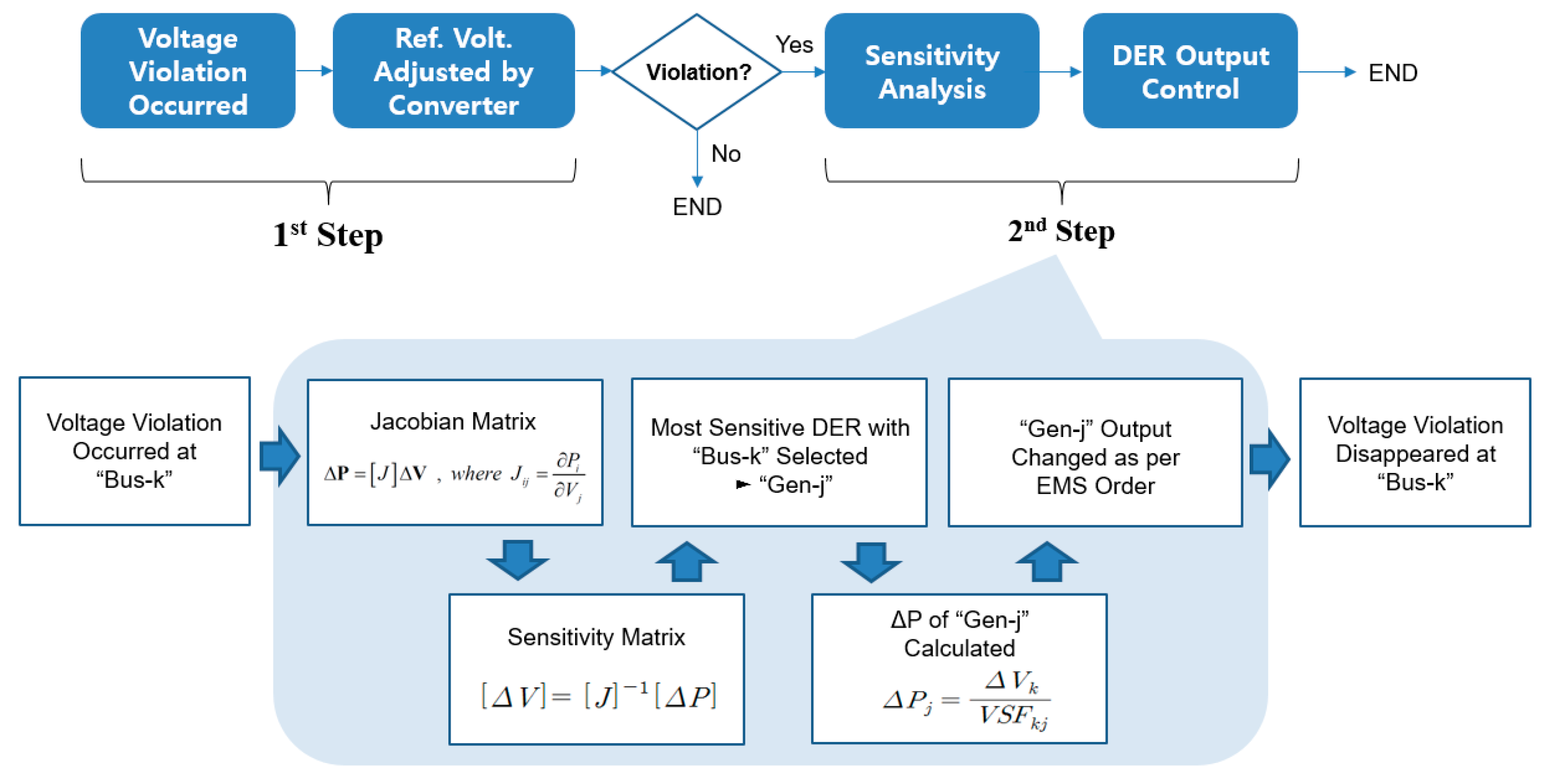
2.2.4. DC Network Voltage Control (DCVC)

The process for voltage control is composed of two stages. The first one is adjustment of the target value for the output voltage of the main converter that operates at a constant voltage. Because there is a certain limit in adjusting the output voltage of the converter, the control of the second stage must be executed if the voltage violation in the power system is not cleared even after the first stage step has been taken. The second one is adjusting the output of the distributed energy resource that is most electrically sensitive to the bus in which the biggest voltage violation occurred, by the amount calculated using the sensitivity factor. Because there is no phase angle or reactive power in DC power systems, voltage has relation only with active power. Therefore, the correlation coefficient between the voltage and the active power output of the distributed energy resource can be obtained through the sensitivity calculation. With utilization of this sensitivity, we can determine how much output of which distributed energy resource to be adjusted to clear the voltage violation. Calculated output adjustment value is transferred to the corresponding distributed energy resource as a command, the output is adjusted accordingly, and then the voltage violation in the power system is cleared. Figure 8 shows the entire flow chart of the voltage control algorithm [31,32,33,34,35].

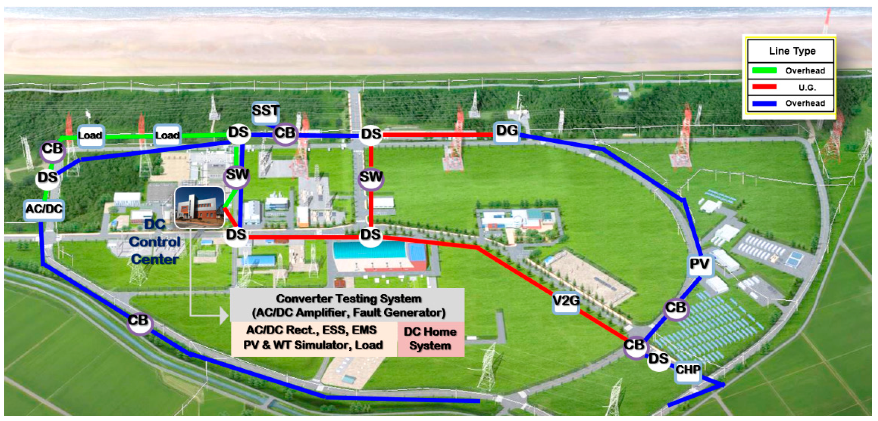
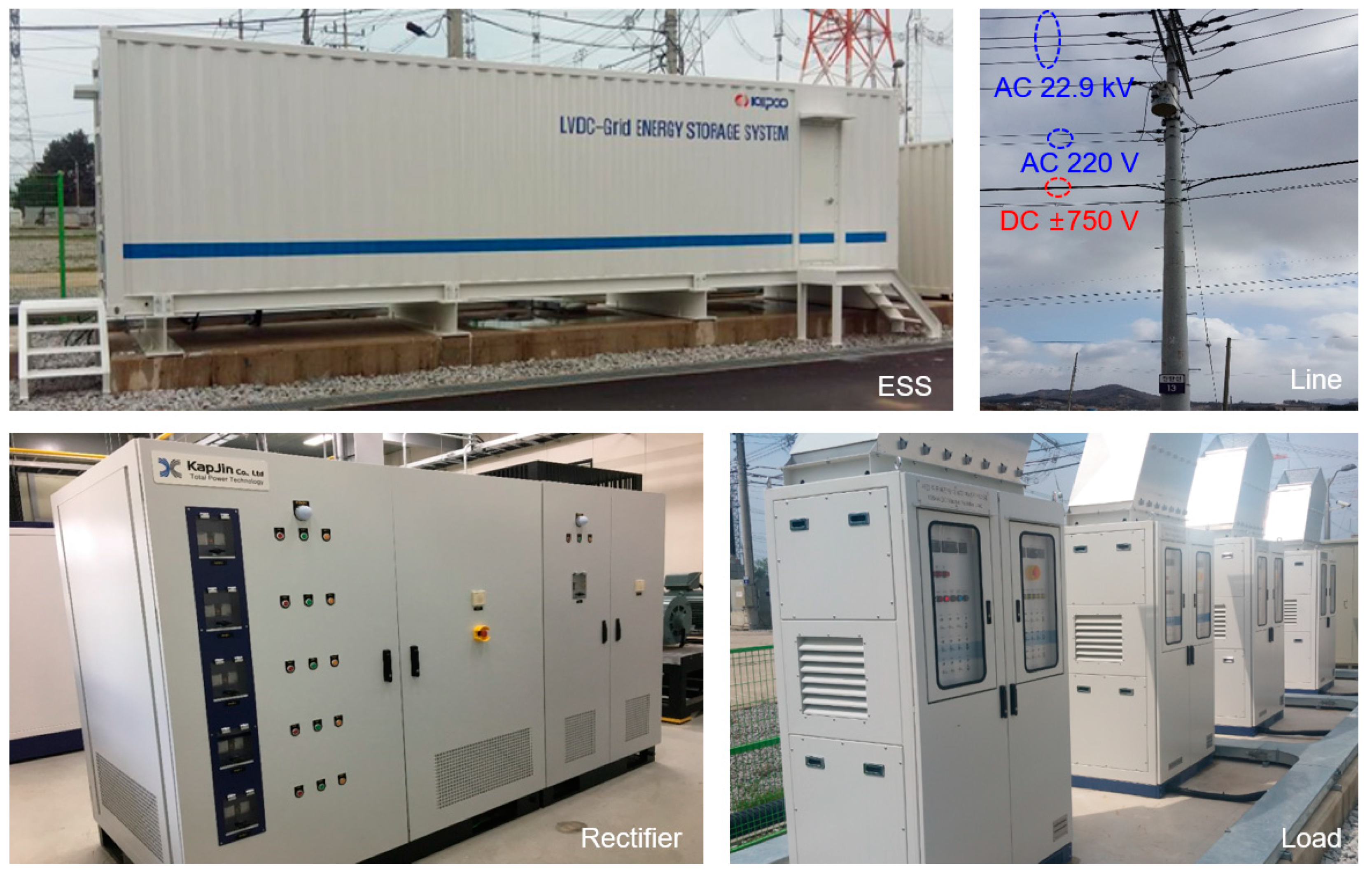
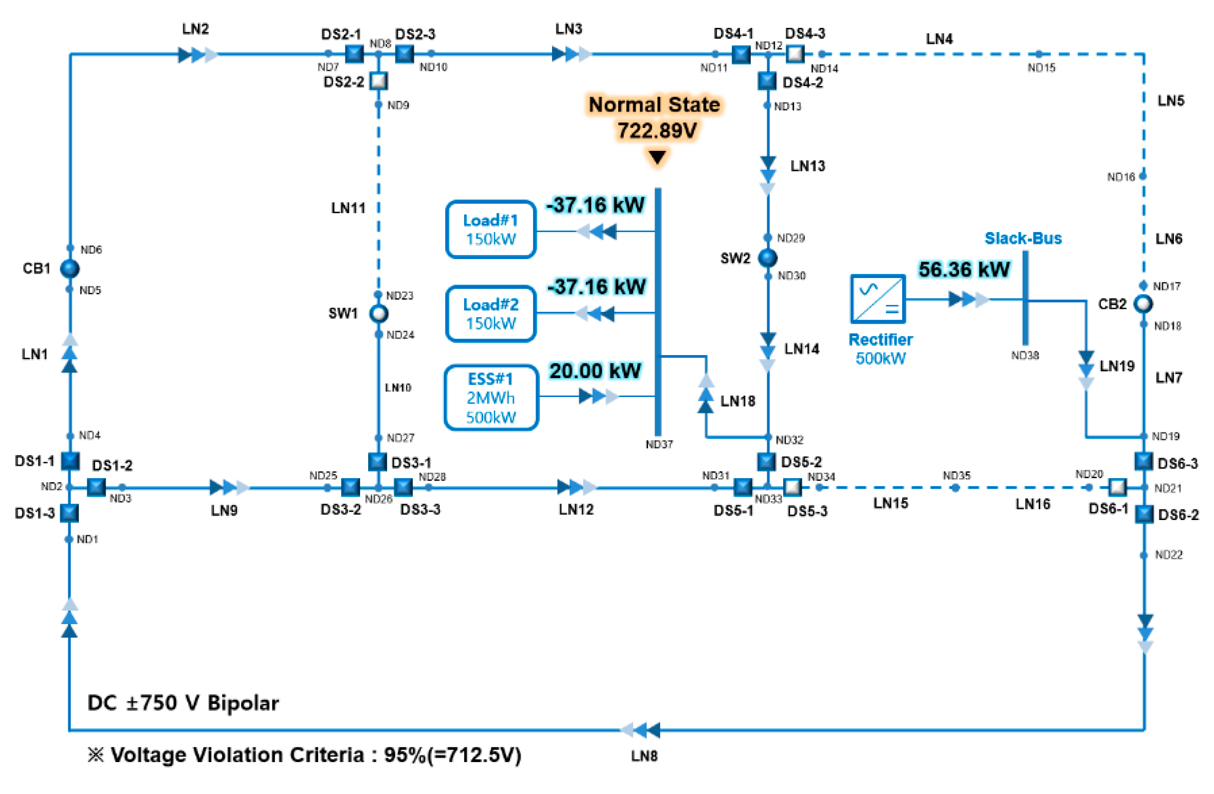
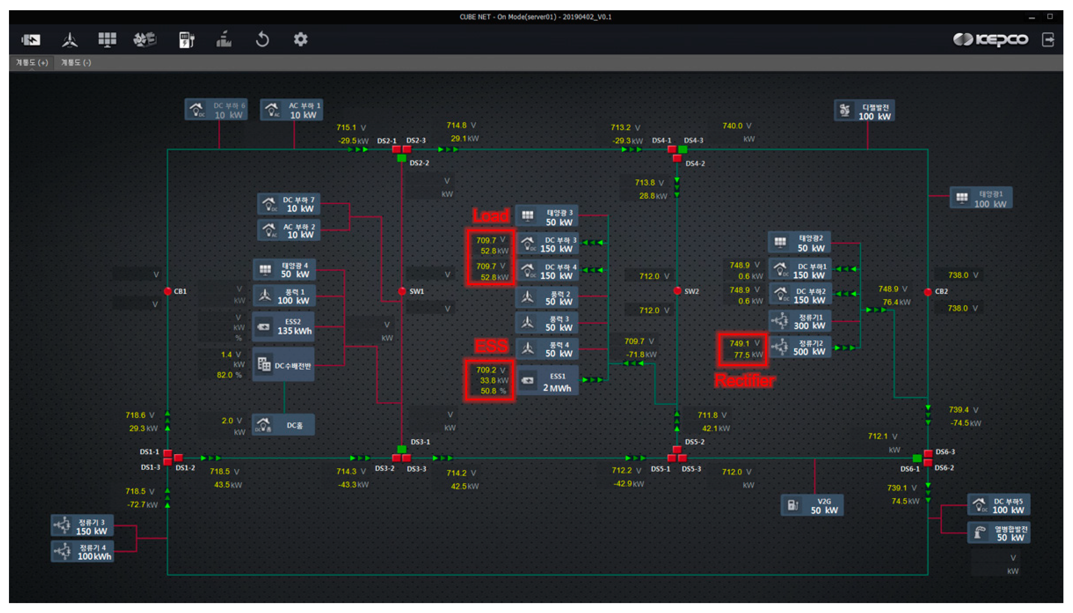
3. Establishment of the Demonstration Site for DC Distribution Networks

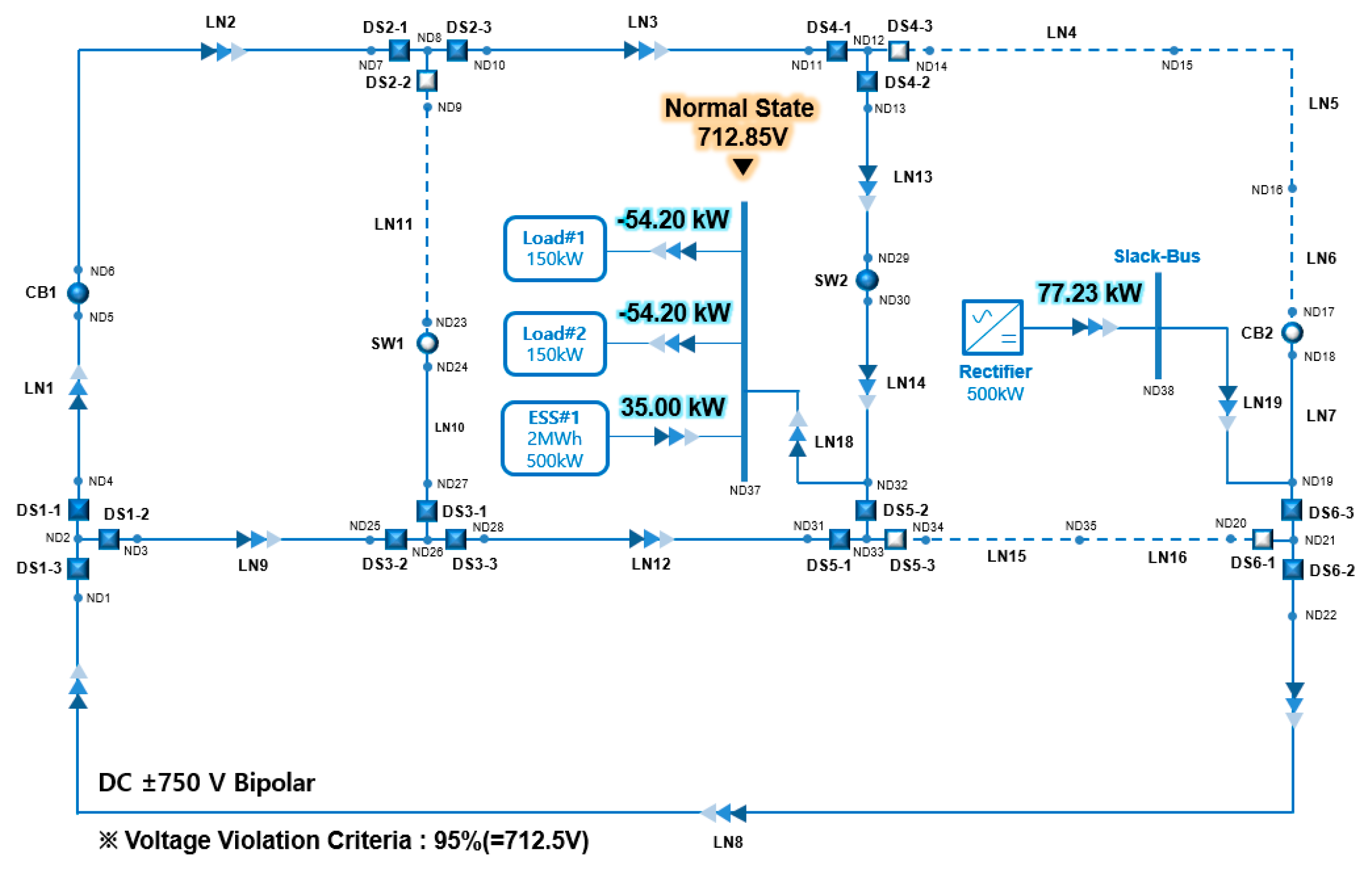
3.1. The Power System and Equipment of the Demonstration Site

Figure 9 is the configuration diagram of the demonstration site for DC distribution at the Gochang Power Testing Center of KEPCO. It is a ±750 V_dc power system composed of overhead and underground cables with a total length of approximately 6 km.

It is composed of a mesh type DC network having a disconnected switch at each branching node so various types of power systems can be configured. Major devices installed include the rectifier with 500 kW ratings for interconnecting with AC 22.9 kV system, ESS (2 MWh) for DC power system interconnection test of distributed energy resources, DC/DC converter (500 kW), and many test loads. The photos in Figure 10 below show the devices installed at the demonstration site.

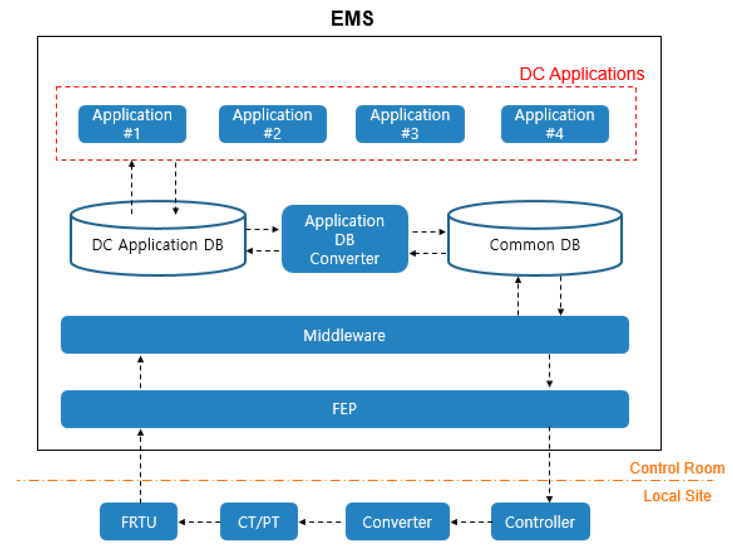
3.2. Establishment of EMS in the Demonstration Site

At the demonstration site, field devices communicate with EMS through the optical ring. Field devices are grouped based on the locations to form network groups, and each network group is connected to the optical cable through a field remote terminal unit (FRTU). Measured data from the measurement devices (current transformer, potential transformer) are transferred to the middleware through optical cable and the FEP of the EMS server (Figure 11).

The middleware works as the route for data transfer, and it reads or writes from/into the common DB as needed. The common DB has been implemented in accordance with IEC-61970 standards. A dedicated DB reflecting DC characteristics is required for the execution of the analysis of DC power system, and a DC application DB has been developed to meet such requirements. Converter software has been implemented to ensure the compatibility with the common DB, and it connects the two DBs to make data exchange possible. Applications read or write data from/into the DC application DB. The results of the applications are transferred to field devices as commands, through the common DB, middleware, FEP, in reverse to the input process. The operator can monitor and control the system through a human machine interface (HMI) interconnected to the common DB.

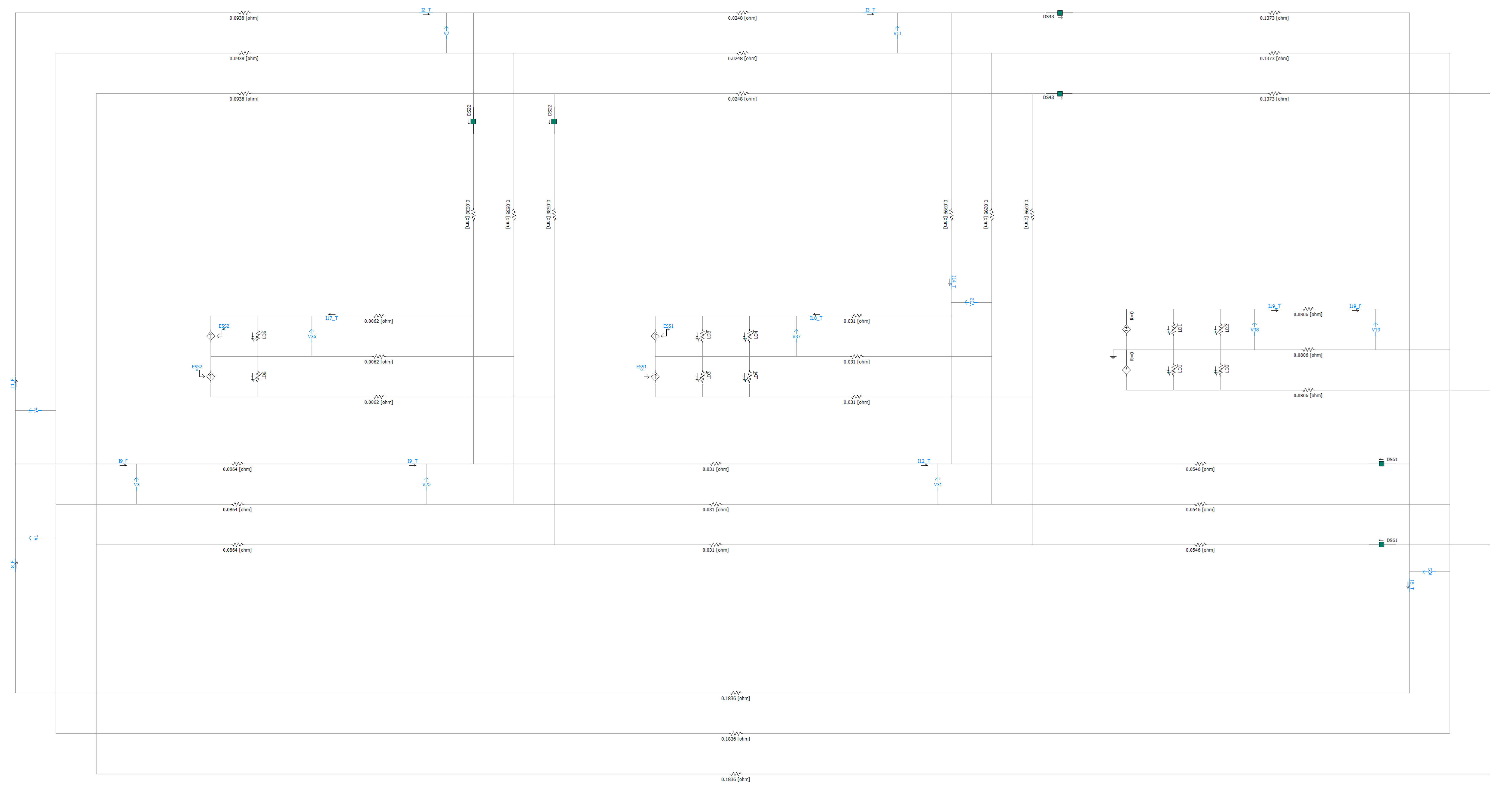
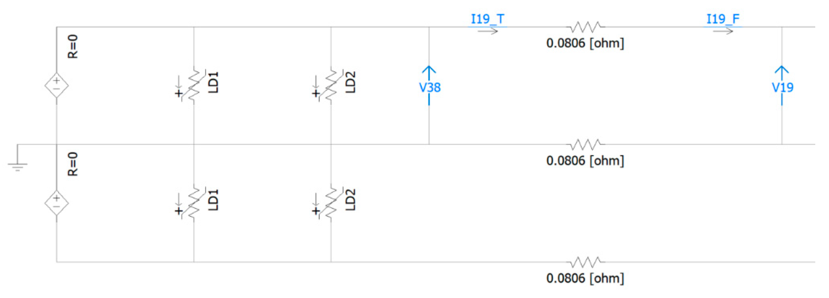
3.3. Configuration of Demonstration Test Equipment

The DC distribution system of the demonstration site is composed of a system with a mesh type as shown in Figure 12, and AC/DC rectifier, distributed energy resource, and simulation load are connected each other, so it is a power system configuration suitable for analyzing the demonstration results of the DC voltage control application based on the power system analysis. The reference converter is a 500 kW rectifier that converts 22.9 kVac into +/−750 Vdc, and it maintains the voltage through DC constant voltage operation. For the DC/DC converter of ESS, both constant voltage and constant current operation are available, however, to avoid the operation conflicts with the rectifier, it has been set to work in constant current mode. Two 150 kW simulation loads composed of resistors were used, and the power consumption varies depending on the voltage. Although there are many other devices in the demonstration site, only those devices mentioned above were used in the test for an effective test.

Figure 12 shows the system diagram and equipment configuration of the demonstration site. Abbreviations used in the system diagram are shown as below. Distributed energy resource, circuit breaker, switch, and disconnected switch can measure the voltage and current and send them to the EMS.

• DC Disconnected Switch (DS)
• DC Line (LN)
• Node (ND)
• DC Switch (SW)
• DC Circuit Breaker (CB)

In case all circuit breakers are closed, the impedance between the AC/DC rectifier and the load gets lower, and voltage violation cannot easily occur, so we configured the system as shown in Figure 12 by manipulating some switches. DS2-2, SW1, DS4-3, CB2, DS5-3, DS6-1 were set to be opened. Solid lines in the figure above mean they are live, while dotted lines mean they are dead.

4. Demonstration Test and Results Analysis

4.1. Configuration of Scenario for the Demonstration Test

To verify the applications executed in the sequence of (DCTP) → (DCSE) → (DCPF) → (DCVC), we made a scenario in which low voltage is cleared by the voltage control command after low voltage is occurred. The demonstration test for voltage control was done using the three scenarios shown below:

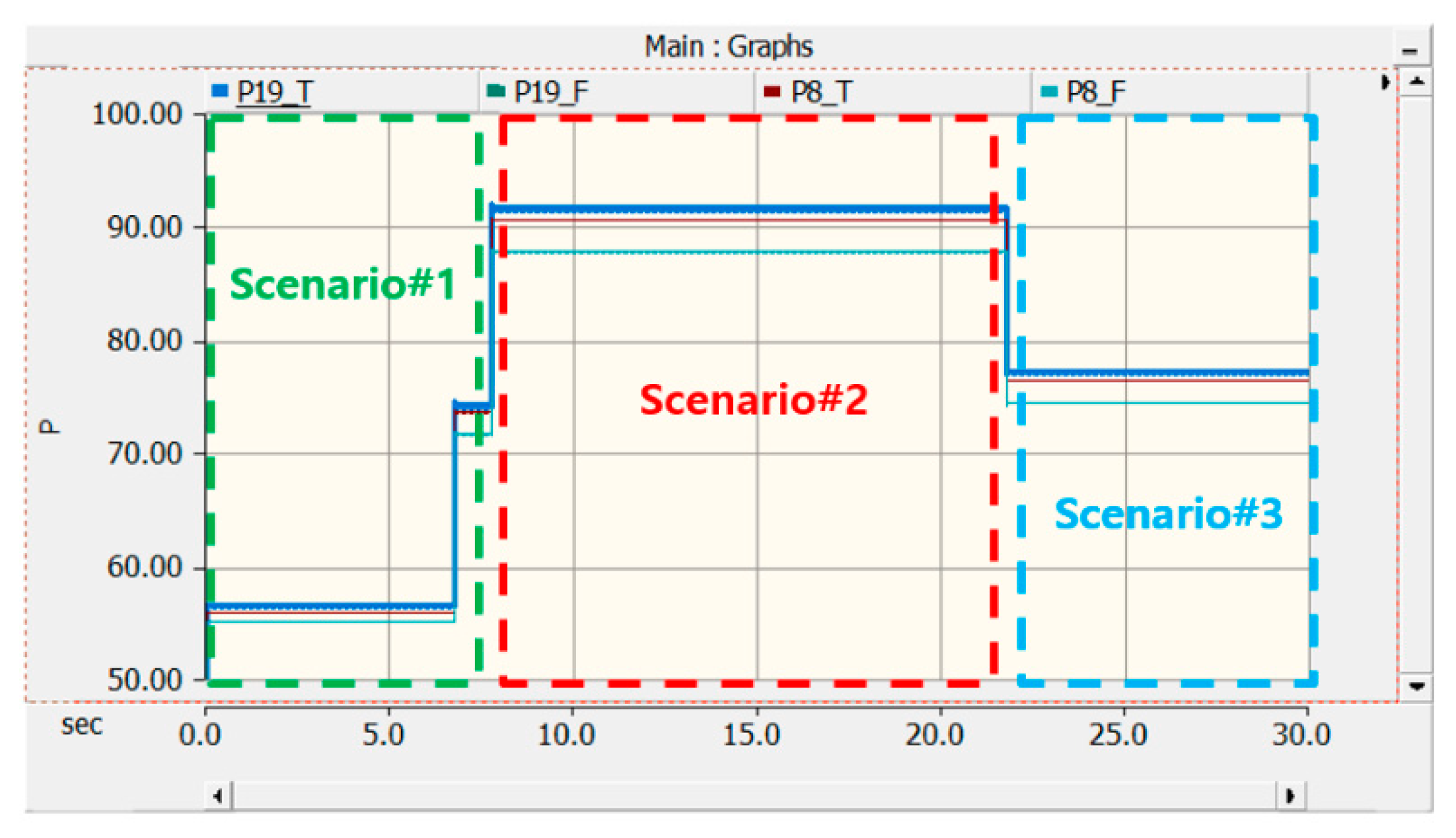
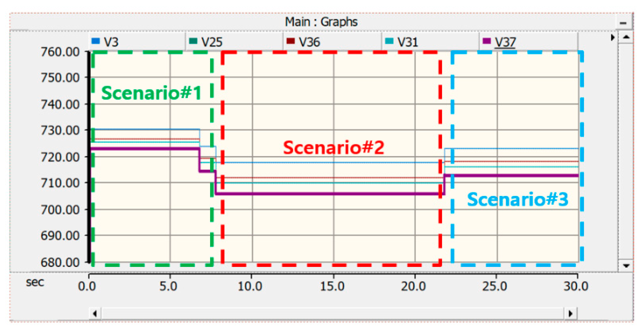
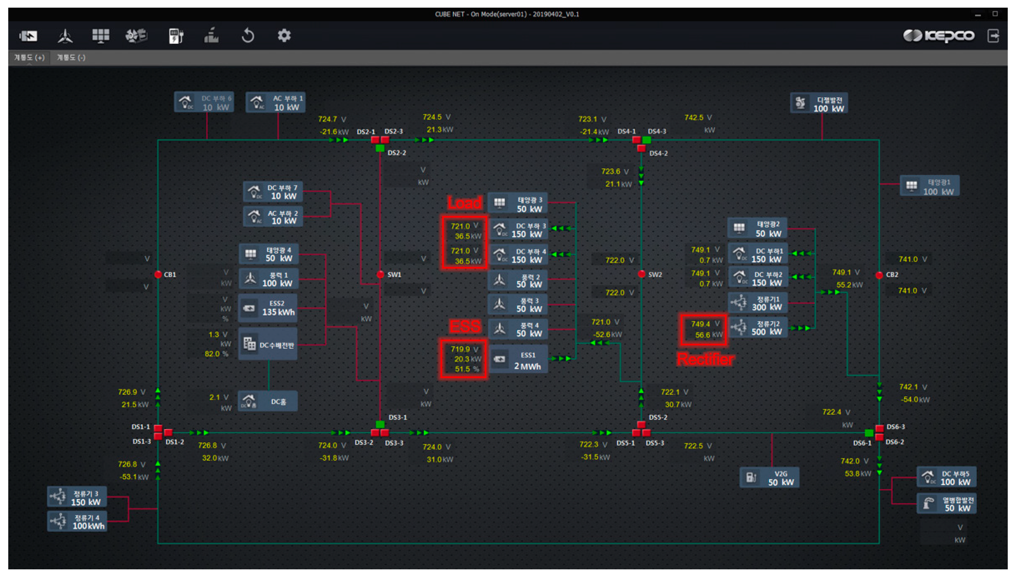
• Scenario #1: No voltage violation (Normal State). Load: 74.32 kW, ESS: 20 kW (Discharge)
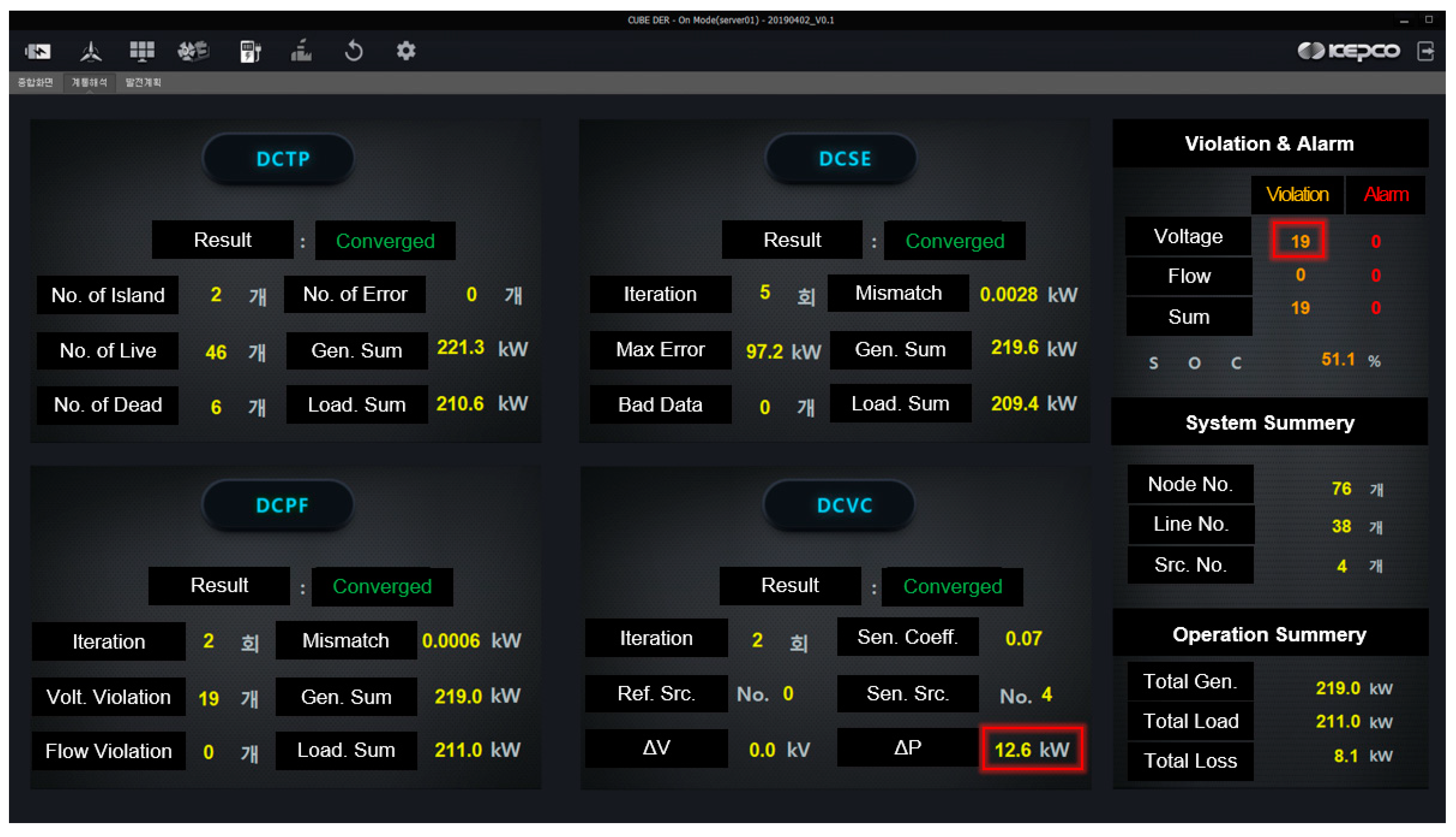
• Scenario #2: Low voltage occurred due to the load increase (Violation State). Load: 106.30 kW, ESS: 20 kW (Discharge)
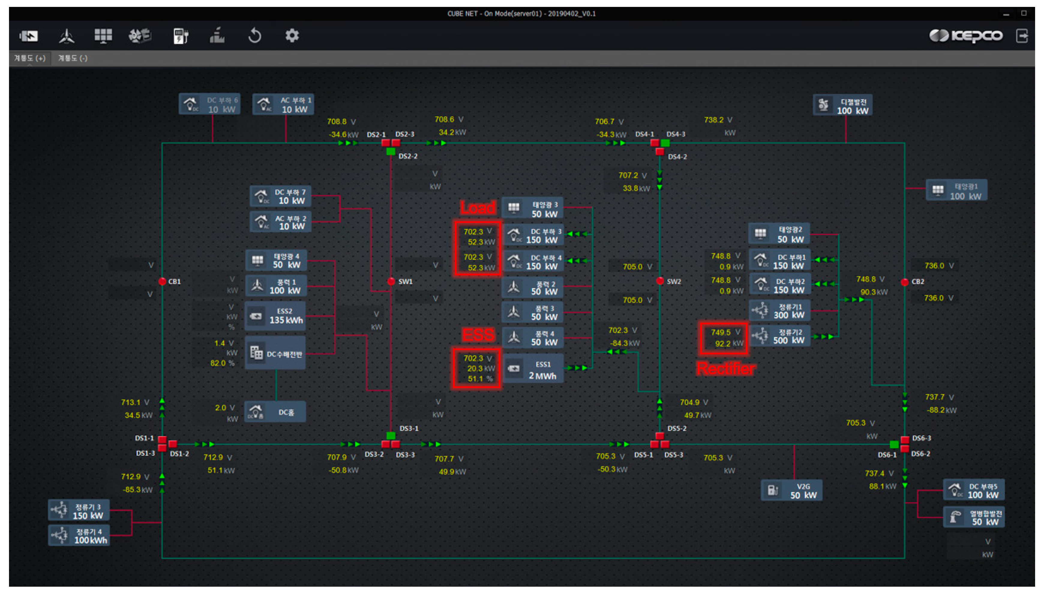
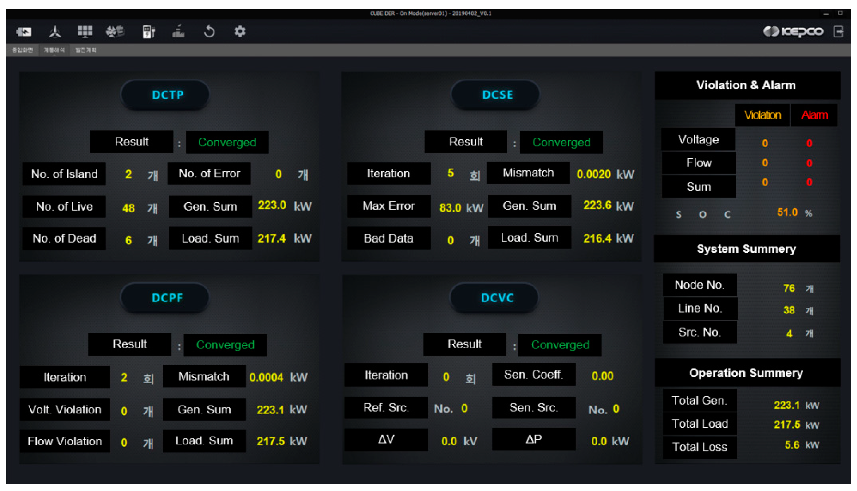
• Scenario #3: Voltage violation was cleared after adjusting ESS output (Normal State)]. Load: 104.40 kW, ESS: 35 kW (Discharge)

Before doing the demonstration test, we modeled the Gochang DC distribution lines using PSCAD/EMTDC (V4.6, Manitoba HVDC Research Centre, Winnipeg, Manitoba, CANADA) to calculate the output of distributed energy resource and simulation load causing voltage violation. Figure 13 shows the Gochang DC power system model made using PSCAD. Because the algorithms of the power system analysis of the applications conduct analysis only for the normal state, we modeled using only the line parameters for R component, not expressing the L and C, for the sake of convenience. The R component of the line was calculated in the way that the resistance of the unit length of line used in the corresponding DC environment was multiplied by the line length. In an ordinary DC power system, the allowable voltage deviation range is ±10%. However, in this case the test was going to take place at field applying actual voltage, so we set the criteria for voltage violation to be ±5% for safety. Therefore, the reference voltage was 750 V, the criteria for over voltage became 787.7 V, and the criteria for low voltage became 712.5 V. Also, for negative pole, the reference voltage was −750 V, the criteria for over voltage became −787.7 V, the criteria for low voltage became −712.5 V. All tests were carried out on the condition that the power should be in a balanced state at each pole. Only the rectifier, ESS, and simulation loads which would be included in the demonstration test were simulated.

As shown in Figure 14, the rectifier modeled as an ideal constant voltage source because the analysis is steady state-based. The simulation loads were modeled as resisters to make them have the same characteristics as actual simulation loads.

Figure 15 shows the modelling of two simulation loads connected to the same node as ESS. In the PSCAD model, ESS was modeled as an ideal constant current source to implement the constant power mode to be used in the demonstration test.

The simulation was carried out for the three scenarios based on the PSCAD model. For the principal points in the power system model, the results were checked by comparing with the measurement values from corresponding volt and ampere meters. Figure 16 shows the change in rectifier output for each scenario.

The slack bus is ND38, and because the rectifier operates in constant voltage mode, the output is automatically calculated depending on the generation, loads and losses in the power system. Figure 17 shows the voltage change for each scenario at ND37 to which ESS is connected.

In Figure 17, Scenario #1 is for normal state, and Scenario #2 is for the situation where the load increased by 40 kW from Scenario #1. We can see that the lowest voltage in Scenario #2 is 705.9Vdc and it is out of the 5% range when comparing with the reference voltage, and there occurs a voltage violation. Scenario #3 is for the situation where the ESS output increases by 15 kW from Scenario #2 and we can see that the voltage has risen from 705.9 Vdc to 712.8 Vdc and it is above the lower limit of the 5% range allowed.

Figure 18Figure 19 and Figure 20 show the situations in the power system diagrams for each scenario. The performance of the applications is verified through the demonstration test carried out at the demonstration site at Gochang under the same conditions based on the results of the simulation.

4.2. Analysis of the Results of the Demonstration Test

4.2.1. Results of the Voltage Control Test

Based on the three configured scenarios, the same power system situations were demonstrated at the demonstration site at Gochang. For Scenario #1, the voltages of all nodes being tested were checked for being within ±5% range based on the results of the power flow calculation after executing the applications in the sequence of (DCTP) → (DCSE) → (DCPF) → (DCVC). The results of the demonstration test are shown in Figure 21 and we can see that the number of voltage violations is zero in the system analysis display. Comparing with the result of the simulation for Scenario #1 with PSCAD, we can see that the values are similar to a certain degree. There may be some deviations due to the control characteristics based on the characteristic of the actual field, synchronizing issues and errors of measurement equipment.

In the system diagram, green lines indicate that they are live, red lines indicate that they are dead. For circuit breakers, however, green color indicates the circuit breaker is open, while red color indicates the circuit breaker is closed.

Figure 22 is the HMI display of EMS for the results of the applications for Scenario #1. We can see that all sequences of (DCTP) → (DCSE) → (DCPF) were converged. In the case of (DCVC), it converged but there is no output displayed because there was no violation.

The system diagram in Figure 23 is the power system demonstration with increased simulation loads according to Scenario #2. In this case, we can also see that the results are similar to those of Scenario #2 with PSCAD.

The figure below is the HMI display of EMS for the results of the applications executed for Scenario #2. We can see that all sequences of (DCTP) → (DCSE) → (DCPF) → (DCVC) were converged. We can also see that voltage control occurred at 19 V violated nodes. (DCVC) calculated the solution to clear the voltage violations. The solution is that the output of the ESS for Source No. 4 must be increased by 12.6 kW and it is shown in Figure 24.

In the case of Scenario #2, the command to for the output of ESS, Source No. 4, was increased by 13 kW. The result is shown in Figure 25.

From the display of power system diagram for Scenario #3 above, we can see that the output of ESS is 33.8 kW, that is, it is increased by approximately 13 kW from the previous value of the 20 kW result of operation in accordance with the calculated DCVC values in Scenario #2. The set values of the simulation loads have not been changed but there are some differences depending on the characteristic of the resistive load which is subjected to voltage.

Figure 26 is HMI display of EMS showing the results of the applications for Scenario #3. As we can see from the display, all of the voltage violations have been cleared and the power system is in normal state again and the DCVC application gives no solution.

We checked the results of the test carried out using the EMS in an actual power system for the three scenarios, based on the results of the PSCAD simulation. The results of the demonstration show patterns that are very similar to those of the simulation, and therefore we can say that the DCVC application has compatibility.

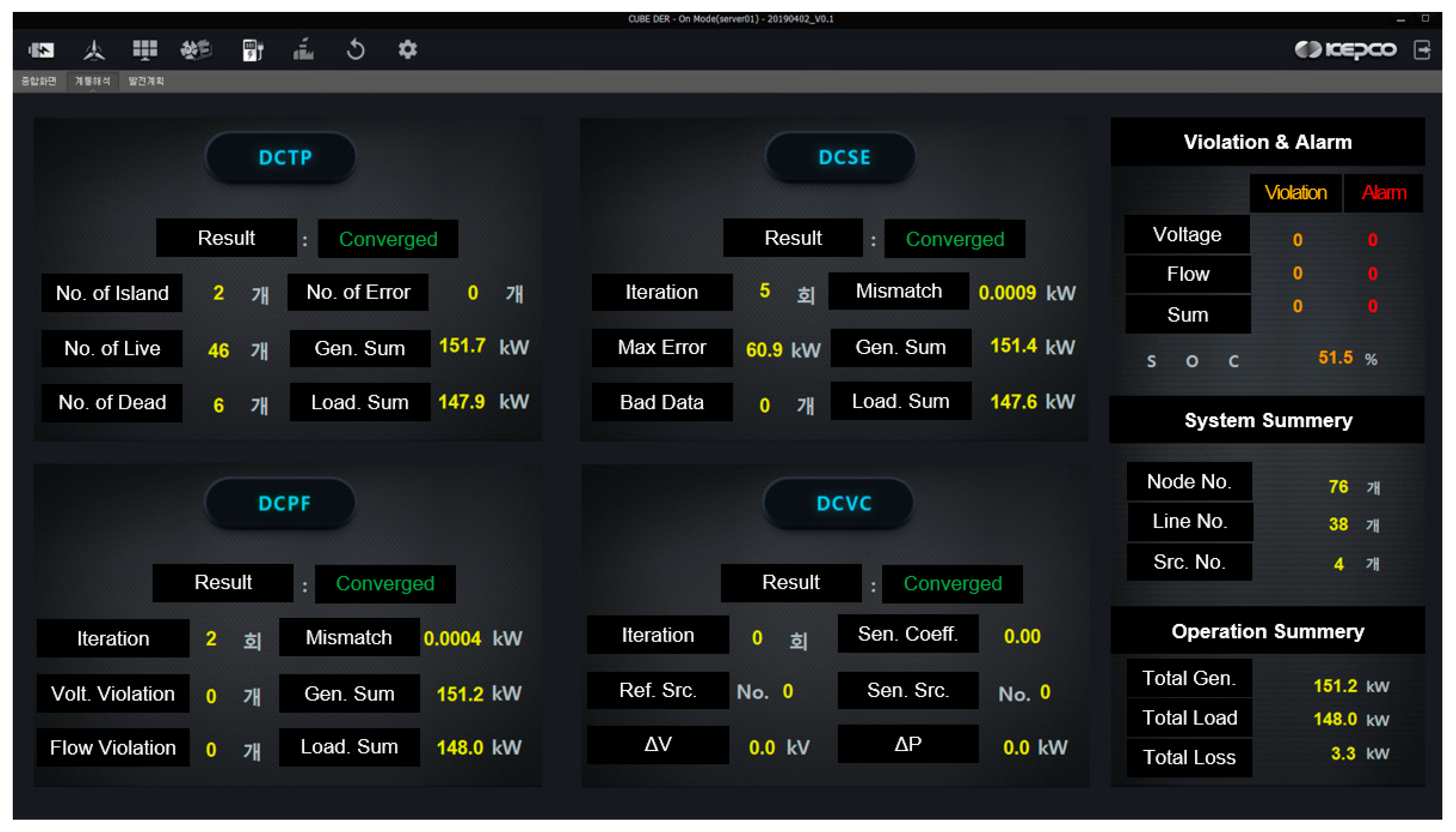
4.2.2. Compatibility Analysis of the Power System Analysis Programs

We converted the demonstration results of three scenarios to CSV format in EMS and compared and analyzed the simulation values of measurement vs. DCSE vs. DCPF vs. PSCAD/EMTDC.

There were measurement values for voltage, and we compared them with the results of simulation and applications for the live nodes. Among the 76 nodes of the DC power system in the demonstration site (38 positive poles and 38 negative poles), we had 30 live nodes for which there were actual measurement devices, data is uploaded to EMS and values of which is not 0 V.

For the power values, the outputs of the sources and loads involved in the test were used for comparison. The sources used for the demonstration test were the ESS (500 kW, 2 MWh) and rectifier (500 kW), and there were four sources in the database for the applications in total because sources were modeled for each pole. For loads, two loads were also used in the test, but in the database, there were four loads in total; two for the positive pole and two for the negative pole. Therefore, comparison of power values was done for the outputs of eight devices in total.

In

Table 3. Demonstration test results of voltage (Scenario #1).

Node No.	Measured Data (Vdc)	(DCSE) Output Data (Vdc)	(DCPF) Output Data (Vdc)	PSCAD/EMTDC (Vdc)	Measured Data & PSCAD/EMTDC Error (%)	(DCSE) Output Data & PSCAD/EMTDC Error (%)	(DCPF) Output Data & PSCAD/EMTDC Error (%)
1-p	726.89	729.94	729.96	730.15	0.4468	0.0283	0.0261
3-p	727.42	729.94	729.96	730.15	0.3735	0.0283	0.0261
4-p	726.99	729.94	729.96	730.15	0.4333	0.0283	0.0261
7-p	724.68	726.95	726.97	727.03	0.3228	0.0111	0.0085
10-p	724.61	726.95	726.97	727.03	0.3329	0.0111	0.0085
11-p	723.32	726.16	726.18	726.21	0.3982	0.0072	0.0046
13-p	723.75	726.16	726.18	726.21	0.3387	0.0072	0.0046
19-p	742.10	743.21	743.22	743.94	0.2471	0.0979	0.0972
22-p	741.90	743.21	743.22	743.94	0.2738	0.0979	0.0972
25-p	724.08	726.46	726.48	726.52	0.3357	0.0086	0.0060
28-p	−727.80	726.46	726.48	726.52	0.1761	0.0086	0.0060
31-p	722.47	725.21	725.23	725.22	0.3786	0.0019	0.0009
32-p	722.00	725.21	725.23	725.22	0.4437	0.0019	0.0009
37-p	721.01	722.97	722.97	722.89	0.2598	0.0105	0.0105
38-p	749.04	749.04	749.04	750.00	0.1285	0.1285	0.1285
1-n	−731.37	−733.57	−733.58	−730.15	0.1675	0.4680	0.4696
3-n	−731.33	−733.57	−733.58	−730.15	0.1613	0.4680	0.4696
4-n	−731.56	−733.57	−733.58	−730.15	0.1927	0.4680	0.4696
7-n	−728.44	−730.50	−730.51	−727.03	0.1938	0.4768	0.4786
10-n	−728.22	−730.50	−730.51	−727.03	0.1637	0.4768	0.4786
11-n	−727.58	−729.68	−729.70	−726.21	0.1884	0.4785	0.4803
13-n	−727.15	−729.68	−729.70	−726.21	0.1300	0.4785	0.4803
19-n	−746.45	−747.18	−747.18	−743.94	0.3372	0.4350	0.4354
22-n	−746.57	−747.18	−747.18	−743.94	0.3534	0.4350	0.4354
25-n	−727.37	−729.99	−730.01	−726.52	0.1165	0.4779	0.4798
28-n	723.94	−729.99	−730.01	−726.52	0.3549	0.4779	0.4798
31-n	−726.43	−728.71	−728.72	−725.22	0.1665	0.4811	0.4831
32-n	−725.99	−728.71	−728.72	−725.22	0.1055	0.4811	0.4831
37-n	−723.88	−726.41	−726.41	−722.89	0.1371	0.4871	0.4871
38-n	−753.15	−753.15	−753.15	−750.00	0.4200	0.4200	0.4200
Average Error (%)					0.2700	0.2506	0.2505

,

Table 4. Demonstration test results of voltage (Scenario #2).

Node No.	Measured Data (Vdc)	(DCSE) Output Data (Vdc)	(DCPF) Output Data (Vdc)	PSCAD/EMTDC (Vdc)	Measured Data & PSCAD/EMTDC Error (%)	(DCSE) Output Data & PSCAD/EMTDC Error (%)	(DCPF) Output Data & PSCAD/EMTDC Error (%)
1-p	713.04	717.32	717.31	717.70	0.6495	0.0528	0.0548
3-p	713.53	717.32	717.31	717.70	0.5816	0.0528	0.0548
4-p	713.04	717.32	717.31	717.70	0.649	0.0528	0.0548
7-p	708.89	712.42	712.37	712.63	0.5253	0.0301	0.0361
10-p	708.53	712.42	712.37	712.63	0.5757	0.0301	0.0361
11-p	706.72	711.12	711.07	711.29	0.6432	0.0241	0.0311
13-p	707.20	711.12	711.07	711.29	0.5755	0.0241	0.0311
19-p	737.70	739.06	739.17	740.15	0.3314	0.1471	0.1323
22-p	737.34	739.06	739.17	740.15	0.3803	0.1471	0.1323
25-p	707.80	711.61	711.56	711.80	0.5621	0.0268	0.0334
28-p	−711.93	711.61	711.56	711.80	0.0185	0.0268	0.0334
31-p	705.17	709.56	709.50	709.69	0.6365	0.0184	0.0266
32-p	704.96	709.56	709.50	709.69	0.6665	0.0184	0.0266
37-p	702.30	705.89	705.74	705.90	0.5105	0.0016	0.0223
38-p	748.77	748.60	748.77	750.00	0.1641	0.186	0.1641
1-n	−717.53	−721.46	−721.31	717.70	0.0231	0.5233	0.5022
3-n	−717.52	−721.46	−721.31	717.70	0.0250	0.5233	0.5022
4-n	−717.63	−721.46	−721.31	717.70	0.0092	0.5233	0.5022
7-n	−712.81	−716.55	−716.38	712.63	0.0248	0.5498	0.5264
10-n	−712.49	−716.55	−716.38	712.63	0.0197	0.5498	0.5264
11-n	−711.01	−715.25	−715.08	711.29	0.0390	0.5567	0.5328
13-n	−710.87	−715.25	−715.08	711.29	0.0597	0.5567	0.5328
19-n	−742.12	−743.21	−743.12	740.15	0.2657	0.4129	0.4015
22-n	−742.05	−743.21	−743.12	740.15	0.2572	0.4129	0.4015
25-n	−711.44	−715.74	−715.57	711.80	0.0508	0.5537	0.5300
28-n	707.62	−715.74	−715.57	711.80	0.5875	0.5537	0.5300
31-n	−709.34	−713.69	−713.52	709.69	0.0487	0.5637	0.5391
32-n	−709.09	−713.69	−713.52	709.69	0.0841	0.5637	0.5391
37-n	−705.52	−710.02	−709.80	705.90	0.0537	0.5834	0.5530
38-n	−752.70	−752.75	−752.70	750.00	0.3599	0.3672	0.3599
Average Error (%)					0.3109	0.2873	0.2776

and

Table 5. Demonstration test results of voltage (Scenario #3).

Node No.	Measured Data (Vdc)	(DCSE) Output Data (Vdc)	(DCPF) Output Data (Vdc)	PSCAD/EMTDC (Vdc)	Measured Data & PSCAD/EMTDC Error (%)	(DCSE) Output Data & PSCAD/EMTDC Error (%)	(DCPF) Output Data & PSCAD/EMTDC Error (%)
1-p	718.60	722.19	722.22	722.79	0.5792	0.0831	0.0787
3-p	719.06	722.19	722.22	722.79	0.5162	0.0831	0.0787
4-p	718.61	722.19	722.22	722.79	0.5778	0.0831	0.0787
7-p	715.17	718.00	718.04	718.57	0.4736	0.0791	0.0740
10-p	714.79	718.00	718.04	718.57	0.5263	0.0791	0.0740
11-p	713.34	716.89	716.93	717.40	0.5662	0.0705	0.0652
13-p	713.79	716.89	716.93	717.40	0.5027	0.0705	0.0652
19-p	739.38	740.75	740.76	741.70	0.3125	0.1282	0.1269
22-p	739.28	740.75	740.76	741.70	0.3269	0.1282	0.1269
25-p	714.30	717.31	717.35	717.83	0.4913	0.0720	0.0667
28-p	−718.17	717.31	717.35	717.83	0.0480	0.0720	0.0667
31-p	712.11	715.56	715.60	716.04	0.5485	0.0665	0.0609
32-p	711.84	715.56	715.60	716.04	0.5859	0.0665	0.0609
37-p	709.79	712.43	712.43	712.85	0.4288	0.0590	0.0590
38-p	748.90	748.90	748.90	750.00	0.1471	0.1471	0.1471
1-n	−722.95	−726.09	−726.09	722.79	0.0217	0.4564	0.4569
3-n	−723.17	−726.09	−726.09	722.79	0.0529	0.4564	0.4569
4-n	−722.91	−726.09	−726.09	722.79	0.0163	0.4564	0.4569
7-n	−719.04	−721.88	−721.89	718.57	0.0653	0.4611	0.4617
10-n	−718.67	−721.88	−721.89	718.57	0.0143	0.4611	0.4617
11-n	−717.35	−720.77	−720.78	717.40	0.0070	0.4700	0.4705
13-n	−717.24	−720.77	−720.78	717.40	0.0227	0.4700	0.4705
19-n	−743.81	−744.73	−744.73	741.70	0.2842	0.4079	0.4080
22-n	−743.62	−744.73	−744.73	741.70	0.2582	0.4079	0.4080
25-n	−717.79	−721.19	−721.20	717.83	0.0063	0.4684	0.4690
28-n	714.17	−721.19	−721.20	717.83	0.5101	0.4684	0.4690
31-n	−716.19	−719.44	−719.44	716.04	0.0214	0.4742	0.4748
32-n	−715.69	−719.44	−719.44	716.04	0.0491	0.4742	0.4748
37-n	−712.76	−716.29	−716.29	712.85	0.0124	0.4824	0.4824
38-n	−752.91	−752.91	−752.91	750.00	0.3875	0.3875	0.3875
Average Error (%)					0.2794	0.2696	0.2679

the measured data, (DCSE) output data, (DCPF) output data and PSCAD/EMTDC (V4.6, Manitoba HVDC Research Centre, Winnipeg, Manitoba, CANADA) simulation results for three scenarios there listed and each data and error is compared and analyzed in the tables based on the result values of the PSCAD/EMTDC simulation.

In the tables above, we can see that the average percentage errors of the three kind of data are within the range of 0.2–0.4%. Also, there are no single data with errors exceeding 1%. This means that the measured data, as well as the results of state estimation and power flow calculation, are very accurate. Because the errors in measured data are very slight, results of the state estimation and power flow which take the measured data as input, are not much different from the measured data. We can see that the errors are getting less in the sequence of measurement > (DCSE) > (DCPF). This may be thought of the phenomenon appeared in the process in which the two programs process the measured data to make them fit the equations of power flow calculation. We can see that the results of the two applications have very slight errors in comparison with the measured data and the results of PSCAD/EMTDC and we can also say, by this, that the two applications have compatibility, and the database work for EMS, PSCAD/EMTDC simulation, and the demonstration test have all been accurately carried out.

Table 6. Demonstration test result of power (Scenario #1).

Equipment	Measured Data (kW)	(DCSE) Output Data (kW)	(DCPF) Output Data (kW)	PSCAD/EMTDC (kW)	Measured Data & PSCAD/EMTDC Error (%)	(DCSE) Output Data & PSCAD/EMTDC Error (%)	(DCPF) Output Data & PSCAD/EMTDC Error (%)
Rectifier (Pos.)	54.20	54.13	54.09	56.36	3.8325	3.9540	4.0355
ESS (Pos.)	20.30	20.40	20.29	20.00	1.5110	1.9875	1.4700
Rectifier (Neg.)	56.00	55.82	55.79	56.36	0.6388	0.9514	1.0092
ESS (Neg.)	20.66	20.72	20.65	20.00	3.2910	3.5960	3.2355
Load#1 (Pos.)	−36.50	−36.32	−36.51	−37.16	1.7874	2.2489	1.7530
Load#2 (Pos.)	−36.50	−36.32	−36.51	−37.16	1.7874	2.2489	1.7530
Load#1 (Neg.)	−37.39	−37.28	−37.41	−37.16	0.6254	0.3280	0.6773
Load#2 (Neg.)	−37.39	−37.28	−37.41	−37.16	0.6254	0.3280	0.6773
Average Error (%)					1.7624	1.9554	1.8264

Table 7. Demonstration test result of power (Scenario #2).

Equipment	Measured Data (kW)	(DCSE) Output Data (kW)	(DCPF) Output Data (kW)	PSCAD/EMTDC (kW)	Measured Data & PSCAD/EMTDC Error (%)	(DCSE) Output Data & PSCAD/EMTDC Error (%)	(DCPF] Output Data & PSCAD/EMTDC Error (%)
Rectifier (Pos.)	91.30	89.31	89.17	91.70	0.4362	2.6108	2.7622
ESS (Pos.)	19.49	19.50	19.28	20.00	2.5730	2.5030	3.6040
Rectifier (Neg.)	89.60	89.50	89.44	91.70	2.2901	2.3960	2.4609
ESS (Neg.)	20.40	20.62	20.52	20.00	2.0075	3.0770	2.5865
Load#1 (Pos.)	−51.88	−51.84	−52.43	−53.15	2.3893	2.4595	1.3582
Load#2 (Pos.)	−51.88	−51.84	−52.43	−53.15	2.3893	2.4595	1.3582
Load#1 (Neg.)	−53.07	−52.51	−52.76	−53.15	0.1550	1.2019	0.7317
Load#2 (Neg.)	−53.07	−52.51	−52.76	−53.15	0.1550	1.2019	0.7317
Average Error (%)					1.5494	2.2387	1.9492

and

Table 8. Demonstration test result of power (Scenario #3).

Equipment	Measured Data (kW)	(DCSE) Output Data (kW)	(DCPF) Output Data (kW)	PSCAD/EMTDC (kW)	Measured Data & PSCAD/EMTDC Error (%)	(DCSE) Output Data & PSCAD/EMTDC Error (%)	(DCPF) Output Data & PSCAD/EMTDC Error (%)
Rectifier (Pos.)	76.60	75.70	75.61	77.23	0.8157	1.9766	2.0939
ESS (Pos.)	33.49	33.43	33.21	35.00	4.3197	4.4900	5.1214
Rectifier (Neg.)	76.40	76.42	76.41	77.23	1.0747	1.0436	1.0562
ESS (Neg.)	34.96	35.08	35.05	35.00	0.1011	0.2206	0.1520
Load#1 (Pos.)	−52.63	−52.73	−53.08	−54.20	2.8899	2.7172	2.0740
Load#2 (Pos.)	−52.63	−52.73	−53.08	−54.20	2.8899	2.7172	2.0740
Load#1 (Neg.)	−54.07	−53.89	−53.93	−54.20	0.2463	0.5677	0.4996
Load#2 (Neg.)	−54.07	−53.89	−53.93	−54.20	0.2463	0.5677	0.4996
Average Error (%)					1.5730	1.7876	1.6963

are for comparison between powers at sources and loads. We can see that, comparing with the case of voltage where they have errors of within 1%, there are errors exceeding 1% for power. For the fact that errors are bigger in the case of power compared with the case of voltage, there may be two reasons. The first one is the accuracy of measurement devices. When seeing the specifications of the measurement devices installed in the fields, the devices for voltage measurement have an accuracy of 0.1%, while the devices for power (current) measurement have an accuracy of 1%. Therefore, we can say that the power values monitored in EMS are 10 times as incorrect when compared with voltage values. The second reason is the weight setting of the state estimation. When setting the weight in state estimation, they put more weight on voltage than power. It means that the power was adjusted more than the voltage to make the results when the contradictory data, not corresponding to the power equation exists. For these two reasons, there are more errors in actual measurement data than voltage values and so do the results of the state estimation and power flow calculation.

5. Conclusions

In this paper, a central control method to maintain the voltage that is an important element in any DC distribution network operation has been proposed. The configuration and sequence of the DC real-time power system analysis applications executed in the central EMS for voltage control were proposed. Algorithms and programs for the four applications; DC topology process (DCTP) for tracing the connections among devices in DC power system and derives the models for analysis, DC state estimation (DCSE) for correcting errors in measured data, DC power flow (DCPF) for the derivation of power flow equations, DC voltage control (DCVC) for the solutions to clear any occurrence of voltage violation have been developed. Voltage violation scenarios for the DC distribution system in the demonstration site were made, applications were loaded in the EMS, and the demonstration test was carried out. Compatibility was verified through comparisons of the measured values, results of applications, and values from PSCAD/EMTDC simulation. The developed applications can be installed in the EMS of any site and used, once the database for the corresponding DC grid is established. It is expected that, even in the DC power systems with complicated mesh structure, the stability of operation would be improved utilizing these applications.

Because the data pre-processing applications with the sequence of (DCTP) > (DCSE) > (DCPF) provide basic data for analysis of the DC power system, they can be utilized as basic programs together with applications with other purposes which might be developed in the future as shown in Figure 27. There are many elements to be considered in the operation of these DC power system such as protection coordination, multi-terminal DC network control, converter droop control and overcurrent control of lines. In the future, we are going to develop various advanced applications needed to ensure the reliability in the operation of the DC distribution network, utilizing previously developed programs.

References

1. Lana, A.; Pinomaa, A.; Nuutinen, P. Control and monitoring solution for the LVDC power distribution network research site. In Proceedings of the IEEE First International Conference DC Microgrids (ICDCM), Atlanta, GA, USA, 7–10 June 2015; pp. 7–10. [Google Scholar]
2. Kaipia, T.; Nuutinen, P.; Lohjala, A. Field test environment for LVDC distribution—Implementation experiences. In Proceedings of the CIRED Workshop, Lisbon, Xi’an, China, 29–30 May 2012. [Google Scholar]
3. Nuutinen, P.; Kaipia, T.; Peltoniemi, P. Research site for low-voltage direct current distribution in a utility network—Structure, functions, and operation. IEEE Trans. Smart Grid 2014, 5, 2574–2582. [Google Scholar] [CrossRef]
4. Dragičević, T.; Lu, X.; Vasquez, J.C. DC microgrids—Part I: A review of control strategies and stabilization techniques. IEEE Trans. Power Electron. 2016, 31, 4876–4891. [Google Scholar]
5. Youngpyo, C.; Hongjoo, K.; Jaehan, K.; Jintae, C.; Juyong, K. Construction of Actual LVDC Distribution Line. Cired Open Access Proc. J. 2017, 2017, 2179–2182. [Google Scholar]
6. Kim, H.; Cho, Y.; Kim, J.; Cho, J.; Kim, J. Demonstration of LVDC Distribution System in Island. Cired Open Access Proc. J. 2017, 2017, 2215–2218. [Google Scholar] [CrossRef] [Green Version]
7. Cho, Y.-S. A Novel Approach to Enhance the Accuracy of Network Topology Optimization. Electr. Power Compon. Syst. 2017, 45, 131–146. [Google Scholar] [CrossRef]
8. Dos Santos, L.T.; Sechilariu, M.; Locment, F. Prediction-based Economic Dispatch and Online Optimization for Grid-Connected DC Microgrid. In Proceedings of the 2016 IEEE International Energy Conference (ENERGYCON), Leuven, Belgium, 4–8 April 2016. [Google Scholar]
9. Luna, A.C.; Diaz, N.L.; Meng, L.; Graells, M.; Vasquez, J.C.; Guerrero, J.M. Generation-Side Power Scheduling in a Grid-Connected DC Microgrid. In Proceedings of the 2015 IEEE International Conference on DC Microgrid (ICDCM), Atlanta, GA, USA, 7–10 June 2015. [Google Scholar]
10. Yun, S.Y.; Chu, C.M.; Kwon, S.C.; Song, I.K.; Hwang, P.I. Development and Test of Smart Distribution Management System. In Proceedings of the 22nd International Conference on Electricity Distribution, Stockholm, Sweden, 10–13 June 2013. [Google Scholar]
11. Qiantu, R.; Guangyu, H.; Shengwei, M.; Qiang, L. Advanced EMS and its application to shanghai power grid. In Proceedings of the IEEE International Conference Electro/Information Technology, Chicago, IL, USA, 17–20 May 2007. [Google Scholar]
12. Liao, Y. Interface paradigms in energy management system. In Proceedings of the IEEE Southeastcon, Huntsville, AL, USA, 22 April 2008. [Google Scholar]
13. Maghsoodlou, F.; Masiello, R.; Ray, T. Energy management systems. IEEE Power Energy Mag. 2004, 2, 49–57. [Google Scholar] [CrossRef]
14. Becker, D.; Falk, H.; Gillerman, J.; Mauser, S.; Podmore, R.; Schneberger, L. Standards-based approach integrates utility applications. IEEE Comput. Appl. Power 2000, 13, 13–20. [Google Scholar] [CrossRef]
15. Sasson, A.M.; Ehrmann, S.T.; Lynch, P.; Vanslyck, L.S. Automatic power system network topology determination. IEEE Trans. Power Appl. Syst. 1973, PAS-92, 610–618. [Google Scholar] [CrossRef]
16. Prais, M.; Bose, A. A topology processor that tracks network modifications over time. IEEE Trans. Power Syst. 1988, 3, 992–998. [Google Scholar] [CrossRef]
17. Allemong, J.J.; Radu, L.; Sasson, A.M. A fast and reliable state estimation algorithm for AEP’s new control center. IEEE Trans. Power Appl. Syst. 1982, PAS-101, 933–944. [Google Scholar] [CrossRef]
18. Garcia, A.; Monticelli, A.; Abreu, P. Fast decoupled state estimation and bad data processing. IEEE Trans. Power Appl. Syst. 1979, PAS-98, 1645–1652. [Google Scholar] [CrossRef]
19. Monticelli, A. Electric power system state estimation. Proc. IEEE 2000, 88, 262–282. [Google Scholar] [CrossRef]
20. Zhong, S.; Abur, A. Auto tuning of measurement weights in WLS state estimation. IEEE Trans. Power Syst. 2004, 16, 2006–2013. [Google Scholar] [CrossRef]
21. Alsac, O.; Vempati, N.; Stott, B.; Monticelli, A. Generalized state estimation. IEEE Trans. Power Syst. 1998, 13, 1069–1075. [Google Scholar] [CrossRef]
22. Castillo, E.; Conejo, A.J.; Pruneda, R.E.; Solares, C. Observability analysis in state estimation: A unified numerical approach. IEEE Trans. Power Syst. 2006, 21, 877–886. [Google Scholar] [CrossRef]
23. Monticelli, A.; Garcia, A. Reliable bad data processing for real-time state estimation. IEEE Trans. Power Appl. Syst. 1983, PAS-102, 1126–1139. [Google Scholar] [CrossRef]
24. Zhuang, F.; Balasubramanian, R. Bad data processing in power system state estimation by direct data deletion and hypothesis tests. IEEE Trans. Power Syst. 1987, 2, 321–327. [Google Scholar] [CrossRef]
25. Glover, J.D.; Sheikoleslami, M. State estimation of interconnected HVDC/AC systems. IEEE Trans. Power Appl. Syst. 1983, PAS-102, 1805–1810. [Google Scholar] [CrossRef]
26. Monticelli, A. State Estimation in Electric Power Systems: A Generalized Approach; Kluwer: Boston, MA, USA, 1999. [Google Scholar]
27. Abur, A.; Exposito, A.G. Power System State Estimation-Theory and Implementation; Marcel Dekker Inc.: New York, NY, USA, 2004. [Google Scholar]
28. Cheng, D.; Zou, J. Power Flow Calculation Method of DC grid with Interline DC Power Flow Controller (IDCPFC). In Proceedings of the IEEE PES Asia-Pacific Power and Energy Engineering Conference (APPEEC), Macao, China, 1–4 December 2019. [Google Scholar]
29. Farooq, R. SMART DC MICROGRIDS: Modeling and Power Flow analysis of a DC Microgrid for off-grid and weak-grid connected communities. In Proceedings of the IEEE PES Asia-Pacific Power and Energy Engineering Conference (APPEEC), Hong Kong, China, 7–10 December 2014. [Google Scholar]
30. Yan, W.; Ding, C.; Ren, Z.; Lee, W.J. A Continuation Power Flow Model of Multi-Area AC/DC Interconnected Bulk Systems Incorporating Voltage Source Converter-Based Multi-Terminal DC Networks and Its Decoupling Algorithm. Energies 2019, 12, 733. [Google Scholar] [CrossRef] [Green Version]
31. Lee, H.; Mok, P.K.; Ki, W.H. A Novel Voltage Control Scheme for Low-Votalge DC Distribution Systems Using MultiAgent Systems. Energies 2017, 10, 41. [Google Scholar]
32. Choi, J.; Jeong, H.; Choi, J.; Won, D.; Ahn, S.; Moon, S. Voltage control scheme with distributed generation and grid connected converter in a DC microgrid. Energies 2014, 7, 6477–6491. [Google Scholar] [CrossRef] [Green Version]
33. Chung, I.Y.; Trinh, P.H.; Cho, H.; Kim, J.Y.; Cho, J.T.; Kim, T.H. Design and Evaluation of Voltage Control Techniques by Hierarchical Coordination of Multiple Power Converters in Low Voltage DC Distribution System. In Proceedings of the Cired Workshop, Helsinki, Finland, 14–15 June 2016. [Google Scholar]
34. Jeong, H.; Choi, J.; Won, D.; Ahn, S.; Moon, S. Formulation and Analysis of an Approximate Expression for Voltage Sensitivity in Radial DC Distribution System. Energies 2015, 8, 9296–9319. [Google Scholar] [CrossRef] [Green Version]
35. Hai, T.P.; Chung, I.Y.; Kim, T.; Kim, J. Coordinated Voltage Control Scheme for Multi-Terminal Low-Voltage DC Distribution System. J. Electr. Eng. Technol. 2018, 13, 1459–1473. [Google Scholar]
Figure 1. Concept of topology process.
Energies 13 04551 g001
Figure 2. Concept of state estimation.
Energies 13 04551 g002
Figure 3. Sequence of a DC network analysis program.
Energies 13 04551 g003
Figure 4. Equations of DC network state estimations.
Energies 13 04551 g004
Figure 5. Flowchart of DC network state estimation.
Energies 13 04551 g005
Figure 6. Equations of DC network power flow.
Energies 13 04551 g006
Figure 7. Flowchart of DC network power flow.
Energies 13 04551 g007
Figure 8. Flowchart of DC network voltage control.
Energies 13 04551 g008
Figure 9. DC Demonstration site at the Gochang Power Testing Center.
Energies 13 04551 g009
Figure 10. DC Components at the DC demonstration site.
Energies 13 04551 g010
Figure 11. DC EMS system configuration.
Energies 13 04551 g011
Figure 12. Network diagram of the DC demonstration site.
Energies 13 04551 g012
Figure 13. PSCAD/EMTDC model for the network of the DC demonstration site.
Energies 13 04551 g013
Figure 14. PSCAD/EMTDC model for rectifier and load.
Energies 13 04551 g014
Figure 15. PSCAD/EMTDC model for ESS and load.
Energies 13 04551 g015
Figure 16. PSCAD/EMTDC simulation result of rectifier output.
Energies 13 04551 g016
Figure 17. PSCAD/EMTDC voltage simulation result.
Energies 13 04551 g017
Figure 18. Scenario #1: normal state (PSCAD/EMTDC result).
Energies 13 04551 g018
Figure 19. Scenario #2: voltage violation state (PSCAD/EMTDC result).
Energies 13 04551 g019
Figure 20. Scenario #3: Violation Removal State (PSCAD/EMTDC Result).
Energies 13 04551 g020
Figure 21. Network diagram in HMI of EMS (Scenario #1).
Energies 13 04551 g021
Figure 22. Application result in HMI of EMS (Scenario #1).
Energies 13 04551 g022
Figure 23. Scenario #2: network diagram in HMI of EMS (Scenario #2).
Energies 13 04551 g023
Figure 24. Application result in HMI of EMS (Scenario #2).
Energies 13 04551 g024
Figure 25. Network diagram in HMI of EMS (Scenario #3).
Energies 13 04551 g025
Figure 26. Application result in HMI of EMS (Scenario #3).
Energies 13 04551 g026
Figure 27. Advanced DC network applications.
Energies 13 04551 g027