Short-Term Net Load Forecasting with Singular Spectrum Analysis and LSTM Neural Networks

Abstract

Short-term electricity load forecasting is key to the safe, reliable, and economical operation of power systems. An important challenge that arises with high-frequency load series, e.g., hourly load, is how to deal with the complex seasonal patterns that are present. Standard approaches suggest either removing seasonality prior to modeling or applying time series decomposition. This work proposes a hybrid approach that combines Singular Spectrum Analysis (SSA)-based decomposition and Artificial Neural Networks (ANNs) for day-ahead hourly load forecasting. First, the trajectory matrix of the time series is constructed and decomposed into trend, oscillating, and noise components. Next, the extracted components are employed as exogenous regressors in a global forecasting model, comprising either a Multilayer Perceptron (MLP) or a Long Short-Term Memory (LSTM) predictive layer. The model is further extended to include exogenous features, e.g., weather forecasts, transformed via parallel dense layers. The predictive performance is evaluated on two real-world datasets, controlling for the effect of exogenous features on predictive accuracy. The results showcase that the decomposition step improves the relative performance for ANN models, with the combination of LSTM and SAA providing the best overall performance.

1. Introduction

Accurate electricity load forecasting is critical for the safe and reliable operation of power systems, as demand and supply need to be in constant equilibrium. Accurate load forecasting is also critical from an economical standpoint, as forecast errors could lead to unnecessary energy purchases, thus provoking market distortions and price spreads between successive markets [1]. The increased penetration of variable renewable energy sources (VREs) in the generation mix over recent years adds another dimension of complexity by introducing uncertainty on the supply side and by further reinforcing the effect of weather, e.g., solar radiation and wind, on the load profile. In turn, this leads to increased imbalance volumes, further affecting subsequent spot electricity prices [2]. The electricity provided by conventional unit shows increased variations, steeper ramps, and shorter peaks, which in turn forces Transmission System Operators (TSOs) to contract costlier, fast-responding reserves. Therefore, increased load uncertainty leads to an overall increase in production cost, further underlining the crucial role of accurate load forecasting in facilitating the ongoing transition towards an emissions-free electricity grid.

Short-term load forecasting, either sub-hourly, hourly, daily, or peak load, is the subject of intense research. Following [3], an important distinction between forecasting techniques and methodologies could be made; the former refers to a group of models belonging to a similar family, such as Autoregressive Integrated Moving Average (ARIMA) [4], while the latter refers to a general solution framework applicable across different families of models. Such frameworks could include feature selection, similar day approach, and hierarchical forecasting, among others. We remark that the focus of this paper is with reference to methodological aspects of load forecasting.

From a modelling standpoint, statistical time series models, such as ARIMA [4,5], and machine learning models, such as Artificial Neural Networks (ANNs) [6,7,8] and Support Vector Machines (SVMs) [9], are amongst the most popular for short-term load forecasting applications. Exponential smoothing model and its different variations, such as double seasonal exponential smoothing models, show good results [10] but are less popular in real-life applications due to their inability to include exogenous features, e.g., weather forecasts. A popular approach amongst researchers and practitioners is to combine different models and methodologies, leading to so-called hybrid approaches. For example, the authors of [11] considered Principal Component Analysis (PCA) and Multiple Linear Regression (MLR) for daily load predictions.

In recent years, Deep Learning models, highly successful for image pattern recognition and Natural Language Processing (NLP) applications, have emerged as formidable candidates for short-term load forecasting applications [12,13]. Specifically, recurrent Neural Networks (RNNs), such as Long Short-Term Memory (LSTM) [14], are a popular choice for time series forecasting, since they are explicitly developed to handle sequential data. An application of various RNNs for predicting several synthetic and real-life time series can be found in [15], with the results being inconclusive as to which architecture is superior for demand forecasting but rather indicating that a case specific approach should be followed. An LSTM forecasting framework is proposed in [16] for residential load prediction, outperforming several benchmark models. The authors of [17] proposed an enhanced LSTM model for electricity consumption forecast of a power system in a metropolitan area in France. A hybrid approach for short-term load forecasting is presented in [18], where the load signal is processed through the utilization of both LSTM and Convolutional Neural Networks (CNNs). In [19], a custom Deep Learning model that combines multiple layers of CNNs for feature extraction, LSTM layers for prediction, and parallel dense Layers for transforming exogenous variables was proposed.

Regardless of the underlying technique selected, an important challenge from a methodological standpoint is dealing with the inherent seasonality patterns. Standard approaches for dealing with single seasonality include Seasonal Exponential Smoothing and Seasonal ARIMA models [4]. Hourly load, however, is a high-frequency time series, governed by multiple seasonal patterns, namely daily, weekly, and yearly. In that regard, traditional approaches have been extended to accommodate for multiple seasonal patterns, such as in double seasonal exponential smoothing [20] or dynamic harmonic regression with Fourier terms [21]. For ANNs in particular, the general consensus is that deseasonalizing prior to training leads to improved performance [22]. Thus, the standard approach is to first remove the seasonality, to model the seasonally adjusted series, to issue a forecast, and to finally reintroduce the seasonality. Another popular approach with ANNs, which aims at reducing the model’s complexity, is the segmentation of the time series into subseries for each hour of the day. A direct forecasting strategy is then deployed, with individual predictions being combined at the end [23].

Time series decomposition comprises an alternative approach of dealing with complex seasonality. First, the original time series is decomposed into several components, either additive of multiplicative, corresponding usually to trend, seasonality (oscillating or periodic components), and random noise. In turn, these components are modeled and forecasted independently, prior to the reseasonalization phase, where they are combined into the final prediction. Notable techniques include Seasonal and Trend decomposition using Loess (STL) [24], which could be extended for multiple seasonalities, trigonometric-based decomposition (TBATS) [25], and Singular Spectrum Analysis (SSA) [26]. In [27], a decomposition-based LSTM model was proposed to deal with multiple seasonal patterns. In that model, the time series is decomposed into various seasonal components, which are used as exogenous regressors in an LSTM. The results indicated that this approach, denoted as Seasonal Exogenous Approach, shows improved performance in predicting homogeneous time series, such as load consumption. SSA has been applied in the energy domain mainly for wind speed forecasting purposes [28,29,30]. In [31], SSA was combined with LSTM along with variational mode decomposition (VMD) and Extreme Learning Machine (ELM) in order to conduct multi-step ahead wind speed forecasting. Similarly, [32] introduced an ensemble model for multi-step ahead wind speed forecasting, based on VMD and SSA, coupled with an LSTM model.

This work proposes a hybrid approach that combines SSA-based decomposition with ANNs for short-term load forecasting. First, the trajectory matrix of the time series is constructed by mapping a sequence of lagged vectors, and Singular Value Decomposition (SVD) is applied. The extracted Principal Components (PCs) are identified as trend, oscillating (periodical) components, and noise. Next, the extracted PCs are used as external regressors in a global forecasting model, consisting of either a Multilayer Perceptron (MLP) or an LSTM network as the predictive layer. Our main goal is to enable the ANN layers to directly learn from the complex seasonal patterns that govern the data-generating process.

We provide empirical results for two datasets, with the first based on data from the Greek Power System and the second being the well-known 2012 Global Energy Forecasting Competition (GEFCom) [33] dataset. We compare our model against a number of statistical and machine learning benchmarks under two frameworks, namely with and without leveraging exogenous features. The reason for this decision is twofold: first, the proposed models can be compared to benchmarks that do not allow for exogenous features, thus offering unbiased comparisons, and second, insight into how the exogenous variables affect the relative performance of the models can be obtained.

The contributions of this paper can be summarized as follows:

• From a methodological standpoint, we propose a hybrid approach to combine time series decomposition with ANNs, which aims to improve individual performance by leveraging seasonal components as external regressors.
• From an application point of view, we provide extensive empirical results against a number of well known benchmarks, with and without using exogenous features, e.g., weather forecasts, thus quantifying the relative importance of adding them. The results are useful for TSOs and other stakeholders (e.g., retailers and aggregators) to improve their load forecasting capabilities, thus enhancing operational management and participation in electricity markets, respectively.

The rest of this paper is organized as follows. Section 2 provides a short technical description of the proposed methods. Section 3 details the experimental design, including datasets, preprocessing, and hyperparameter tuning. Finally, the results are presented in Section 4, and conclusions are drawn in Section 5.

2. Methodology

The following section provides a short description of the methods employed in this work. Both the basic SSA algorithm and the LSTM network, including the process of combining them, are presented briefly. A description of the standard MLP network is omitted, and we refer to [6] for a comprehensive description of simple feed-forward ANNs for time series forecasting.

2.1. Singular Spectrum Analysis

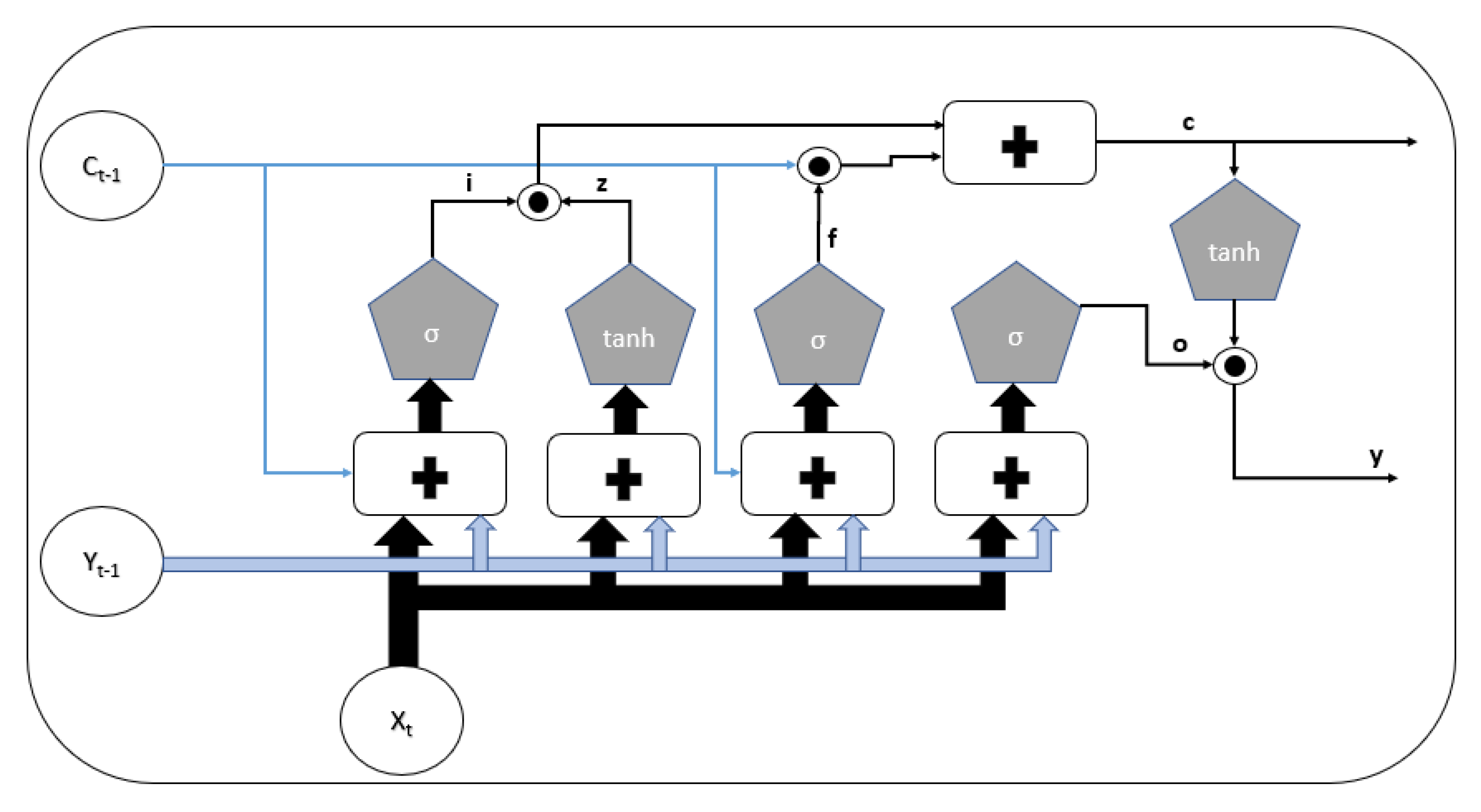
SSA [34] is a nonparametric spectral estimation method that combines elements of time series analysis, dynamical systems, and signal processing. Its roots can be traced in the classical spectral decomposition and the embedding theorem [35]. In practice, it is highly applicable in smoothing and forecasting applications. The basic form of SSA comprises two sequential stages, namely the decomposition stage and the reconstruction stage [36].

First, the time series is decomposed into several components that can be identified as trend, oscillating, and noise. Initially, at the embedding step, the univariate time series is mapped in a sequence of lagged vectors given a selected window length or embedding dimension d, thus obtaining the trajectory matrix, which has the properties of a Hankel matrix, i.e., the elements on the antidiagonal are equal. Let $X=(x_1,x_2,\dots ,x_N)$ be a real-valued time series of N observations, and L be the length of the selected window. The so-called trajectory matrix is obtained as follows:

$$\begin{array}{cc}\hfill & \mathbf{X}={[X_1:\dots :X_K]}^{\prime }=\left[\begin{array}{cccc}{x}_1& x_2& \cdots & x_L\\ x_2& x_3& \cdots & x_{L+1}\\ ⋮& ⋮& \ddots & ⋮\\ x_K& x_{K+1}& \cdots & x_n\end{array}\right],\hfill \end{array}$$

(1)

where $K=n-L+1$ are the lagged vectors selected. Subsequently, the trajectory matrix is decomposed via SVD, resulting into a sum of rank-one bi-dimensional matrices as follows:

$$\begin{array}{cc}\hfill & \mathbf{X}=\sum _{i=1}^d{X}_i=\sum _{i=1}^d\sqrt{{\lambda }_i}{U}_i{V}_i^{{}^{\prime }},\hfill \end{array}$$

(2)

where ${\lambda }_i$, $U_i$, and $V_i$ denote the ith eigenvalue, left singular vector, and right singular vector, respectively, in descending order of magnitude. The collection $({\lambda }_i$, $U_i$, $V_i$) is called the eigentriple of the array X.

At the subsequent reconstruction stage, the goal is to reconstruct the original time series into additive components. Although this step was not employed in the final version of the proposed model, it is presented in order to provide a comprehensive overview of the SSA. First, the grouping step consists of partitioning the extracted PCs produced by the SVD and summing them within each group. The set of indices $J=\{1,\cdots ,L\}$ is partitioned into m disjoint subsets $I_1,\cdots ,I_m$, with each one consisting of a group of p indices $I=\{i_1,\cdots ,i_p\}$ via a process called eigentriple grouping. The matrix $X_I$ is a resultant matrix, hence the decomposition can be denoted as follows:

$$\begin{array}{cc}\hfill & \tilde{X}=\sum _{l=1}^m{X}_{I_l}.\hfill \end{array}$$

(3)

Finally, the diagonal averaging procedure linearly transforms matrix $\tilde{X}$ into a time series $x_0^{*},x_1^{*},x_{N-1}^{*}$, by applying (4) to each array $X_I$. Thus, the original time series is decomposed into a sum of m recreated time series by applying the following:

$$x_k^{*}=\left\{\begin{array}{cc}\frac{1}{k}{\displaystyle \sum _{j=1}^k}\left({\tilde{x}}_{j,k-j+1}\right)\hfill & \mathrm{for}0\le k\le L^{*}\hfill \\ \frac{1}{L^{*}}{\displaystyle \sum _{j=1}^{L^{*}}}\left({\tilde{x}}_{j,k-j+1}\right)\hfill & \mathrm{for}{L}^{*}\le k\le K^{*}\hfill \\ \frac{1}{N-k+1}{\displaystyle \sum _{j=k-K^{*}+1}^{N-K^{*}+1}}\left({\tilde{x}}_{j,k-j+1}\right)\hfill & \mathrm{for}{K}^{*}\le k\le N.\hfill \end{array}\right.$$

(4)

The original time series is finally expressed as a sum of m reconstructed time series as follows:

$$x_n=\sum _{k=1}^m{\tilde{x}}_n^{\left(k\right)}.$$

(5)

2.2. LSTM

As mentioned, RNNs are designed to effectively model dynamics in sequential data. Their design is based on the recursive computation of new states, using the previous states and inputs. However, they are prone to suffering from the vanishing or exploding gradient descent problem during back propagation training [15]. The LSTM network [14] offers a solution to this problem by employing a gated recurrent unit and by keeping a constant error flowing back through time. This section briefly details the basic LSTM architecture (Figure 1), which is the most commonly used, following the notation from [37].

Considering $X=[x_1,\cdots ,x_t]$ to be the input vector, the vector formulas that define a forward pass to update the cell state are computed as follows:

$$\begin{array}{cc}\hfill & z^t=g(W_z{x}^t+R_z{y}^{t-1}+b_z)\hfill \end{array}$$

(6)

$$\begin{array}{cc}\hfill & i^t=\sigma (W_i{x}^t+R_i{y}^{t-1}+p_i\odot c^{t-1}+b_i)\hfill \end{array}$$

(7)

$$\begin{array}{cc}\hfill & f^t=\sigma (W_f{x}^t+R_f{y}^{t-1}+p_f\odot c^{t-1}+b_f)\hfill \end{array}$$

(8)

$$\begin{array}{cc}\hfill & c^t=z^t\odot i^t+c^{t-1}\odot f^t\hfill \end{array}$$

(9)

$$\begin{array}{cc}\hfill & o^t=\sigma (W_o{x}^t+R_o{y}^{t-1}+p_o\odot c^t+b_o)\hfill \end{array}$$

(10)

$$\begin{array}{cc}\hfill & y^t=h\left(c^t\right)\odot o^t,\hfill \end{array}$$

(11)

where $\sigma$, g, and h are point-wise nonlinear activation functions. For the first case, a sigmoid function $\left(\sigma \right)$ is used, while for the other two activation functions, the hyperbolic tangent ($tanh$) is utilized. The notations $W,R,p$, and b refer to input, recurrent, peephole, and bias weights, respectively, with ⊙ denoting the vector pointwise multiplications.

By examining the block’s architecture as showcased in Figure 1, three gates are observed, namely the Input, Forget, and Output gates. Each gate has a unique purpose and depends on the current external input $x^t$ and the previous cell’s output $y^{t-1}$. The Input gate (7) decides how much the cell state would be updated by the block input. The Forget gate (8) decides what information, propagated by the previous cell state, should be discarded. The Output gate (10) selects which part of the cell state should be delivered to the output. Then, the calculation of the block output (11) takes place by multiplying the output gate with the filtered current cell state (9).

2.3. Combining SSA and LSTM

The final model combines SSA-based decomposition with LSTM. Considering an observation at time t, the process is described as follows:

(1)

Let $\{x_t,x_{t-1},\cdots ,x_{t-d}\}$ be the input vector, where d is the embedding dimension selected. Therefore, this input vector corresponds to a new row in the trajectory matrix as defined in (1).

(2)

This vector is subsequently mapped onto the principal axes by means of linear transformation, as obtained by applying SVD (2) to the training dataset.

(3)

The transformed rows are finally fed into the prediction layer, which performs multi-step ahead prediction, thus producing a vector $\{y_{t+1},y_{t+2},\cdots ,y_{t+24}\}$.

The overall process is detailed in the flowchart presented in Figure 2.

The above steps comprise the so-called univariate case, where no exogenous variables are employed. For the case in which exogenous variables are included, denoted as multivariate, after testing various different combinations, an approach similar to [19] is followed, where the exogenous variables are first transformed via parallel a dense (MLP) layer. The output and the PCs of historical load are then concatenated before being used as input to the prediction layer. The final architecture is the result of a long process of trial and error. Two issues warrant a brief discussion; first, the selection of the embedding dimension d; second, why all of the PCs are used as external regressors, instead of performing feature selection.

Regarding the embedding dimension d, it is well-known that hourly load time series is governed by daily and weekly seasonality, which correspond to historical lags 24 and 168, respectively. Initial trials indicated that increasing the embedding dimension beyond lag 168 provided a negligible effect on the PCs, which remained almost identical. Furthermore, the model’s predictive performance remained the same or even declined in some cases, while increasing the computational cost and memory requirements. Therefore, the embedding dimension is set as $d=168$ throughout.

Concerning the selection of PCs, the first PCs explain a great proportion of the variability found in the data. Thus, it is reasonable to reduce the dimension of the input vector by selecting only a number of PCs that exceed a predefined threshold of explained variance. For the case of Greek System Load, specifically, the first eight PCs explained over 90% of the variance found, as shown in Figure 3. Nevertheless, initial results with feature selection were mixed, and in many cases, the predictive performance diminished. Therefore, instead of performing feature selection, we opted for retaining all of the PCs after the decomposition and for carefully applying regularization to avoid overfitting.

3. Experimental Setting

In this section of the paper, a description of the datasets and the subsequent preprocessing analysis used for experimentation of the proposed method are presented. Afterwards, the hyperparameter tuning approach used to fine-grain the performance of the ANNs is introduced. Finally, we provide details regarding the benchmark models considered.

3.1. Datasets

An evaluation was conducted on two datasets. The first comprises of $N=$ 16,056 observations of System Load and weather forecasts for the Greek Power System, spanning the period from July 2017 to May 2019. System load refers to the aggregated electricity load minus the distributed VRE generation, which comprises mostly PV plants. Hence, the daily profile of the System Load is highly dependent upon solar radiation. The weather data comprise day-ahead hourly forecasts for temperature, wind speed, solar radiation, and cloud coverage from different weather stations across Greece. Since it is not the current focus, the problem of how to select weather substations is left for future work [38]. Instead, weather forecasts are aggregated via weighted mean according to the relative contribution of adjacent HV substations to the aggregated System Load. An exception was made for solar radiation predictions, which are aggregated via weighted mean based on approximate capacity of PVs installed in the adjacent area. The second dataset is the GEFCom 2012 dataset, comprising 4 years of hourly measurements (2004–2007) of electricity load from a US energy supplier. Besides the energy forecasting competition, it has also been used in [39] for modelling the recency effect of the temperature and in [15] for comparing various RNNs, among others. Here, performance is assessed on the aggregated demand (Zone 21). Furthermore, we utilized temperature measurements available. Note that, in this case, the forecasts are considered ex post rather than ex ante, as in the case of the Greek System Load, since the true temperature is used.

3.2. Preprocessing

A preliminary analysis is conducted prior to training. For the Greek System Load in particular, visual inspection indicates signs of heteroskedasticity; thus, a logarithmic transformation is applied. Figure 4 plots the average daily profile for the Greek System Load, calculated over the course of one month; hours from 6 am up to 6 pm experience higher variance, which is mitigated when the logarithmic transformation is applied. This increased variance could be partially attributed to the effect of solar generation on System Load. Furthermore, Figure 5 showcases the nonlinear effect of solar radiation and temperature on System Load, which justifies including these features as external regressors.

Overall, both time series were processed as following: first, a logarithmic transformation was applied to mitigate the heteroskedasticity effects, and second, the observations were scaled linearly in the range $[0,1]$. Furthermore, the weather variables were also scaled prior to training. For models that were trained with seasonally adjusted data, an extra preprocessing step was included. Specifically, the daily and weekly seasonal components were removed via differencing (at lags 24 and 168, respectively) prior to scaling and model training. The seasonal differencing step was reversed after the predictions were issued.

3.3. Hyperparameter Tuning

Finding an optimal configuration of hyperparameters for the ANNs is crucial to attain good predictive performance. First, we defined the search space for the required hyperparameters. Then, a meta-optimization algorithm was employed in order to obtain a locally optimal configuration. Popular algorithms include grid search, random search, and Bayesian optimization techniques. In this work, the random search algorithm [40] was selected, which outperforms grid search when the search is confined in the search space.

Specifically, the learning rate $\eta$ was sampled uniformly from the discrete space $\{{10}^{-1},{10}^{-2},$${10}^{-3}\}$. The number of nodes in the hidden layer, denoted $N_h$, was selected from the space $[N/2,2N]$, where N denotes the size of the input vector. Regarding the activation function of the MLPs, sigmoid, hyperbolic tangent ($tanh$) and the rectifier linear unit ($ReLU$) are considered for selection. In all cases, training is conducted for up to 1000 epochs, using an early stopping algorithm that assesses performance in a validation set. The early stopping algorithm effectively acts as a regularizer, thus protecting against overfitting. The Stochastic Gradient Descendent (SGD) algorithm is used for training, employing a mean absolute error loss function. All of the ANN models were developed in Python, using the Keras library [41] with Tensorflow as the backend. In total, 300 parameter configurations were tested at each case. After tuning, the model was re-trained with 10 random weight initializations. The weights of the best-performing model were subsequently retrieved, and the forecast on the test set was conducted.

3.4. Benchmark Models

The proposed approaches suggest combinations of SAA with either LSTM (LSTM-SSA) or MLP (MLP-SSA). The following benchmarks were also considered: standard MLP and LSTM without deseasonalization, and seasonally adjusted MLP and LSTM, denoted as MLP-Deseason and LSTM-Deseason, respectively. In all cases, the ANNs follow a Multiple Input Multiple Output (MIMO) strategy [23], thus forecasting the whole horizon in one shot. For the seasonally adjusted models, a similar approach to [15], i.e., seasonal differencing, is followed.

The main purpose of this section is to showcase that the SSA decomposition improves ANNs’ performance; therefore, the simple MLP could be considered our base case. However, in order to present a more comprehensive study, a number of additional benchmark models are considered, namely ARIMA using a direct modelling approach, i.e., 24 models for each hour of the day, multiple STL decomposition with exponential smoothing for prediction [24], nonlinear autoregressive regression (NAR), and SVM. The first three were developed in R using the forecast package [42].

As mentioned above, we evaluated performance under two frameworks: at first using only historical load, which refers to the univariate case and afterwards including the external variables available, i.e., the multivariate case. The justification behind this decision is that, since some benchmark methods do not allow for exogenous features or require detailed modeling in order to adequately capture nonlinear effects of weather variables (see for example Figure 5), a level playing field is provided. Furthermore, since this work is mainly focused on ANNs, the multivariate case is restricted only to ANN-related models. Finally, this distinction provides a better sense of how the weather variables affect the relative performance by comparing the both cases.

Predictive performance was assessed on day-ahead hourly predictions. Since the target values are significantly greater than zero in both cases, the Mean Absolute Performance Error (MAPE) is an appropriate selection for measuring the forecasting error. The MAPE is defined as follows:

$$\begin{array}{cc}\hfill & MAPE=\frac{100\%}{N}\sum _{t=1}^N\left|\frac{y_t-\widehat{y_t}}{y_t}\right|.\hfill \end{array}$$

(12)

where N denotes the number of forecasted points, $y_t$ denotes the actual value, and $\widehat{y_t}$ denotes the forecasted value.

Furthermore, we apply pairwise Diebold–Mariano (DM) [43] statistical tests to assess the significance of the results. Provided two sets of forecasts derived from different forecasting models, the DM test checks the null hypothesis that both sets of forecasts have equal predictive accuracy against the alternative hypothesis that one of the models outperforms the other. This result provides helpful insights and complements standard error metrics such as MAPE.

4. Results

This section presents the results for the two datasets considered: the Greek System Load and the GEFCom dataset. During the validation procedure, we observed that the learning rate was the most important hyperparameter while the results were generally insensitive to the number of nodes in the hidden layer. This could be attributed to the effect of the early stopping algorithm implemented during training, which adapts itself to the underlying model architecture. Throughout, $\eta$ was set at ${10}^{-3}$, while the number of nodes and the activation functions varied for each case.

4.1. Greek System Load

For the Greek System Load, hourly observations from 07/2017 to 01/2019 comprise the training set, with observations from 01/2019 to 05/2019 comprising the test set. The first two columns of

Table 1. MAPE results for the examined use cases.

Use Case	Greek System Load		GEFCom
Models	Univariate	Multivariate	Univariate	Multivariate
ARIMA	6.60	-	7.19	-
STL	5.92	-	6.19	-
NAR	6.79	-	7.08	-
SVM	7.31	-	6.98	-
MLP	5.91	3.99	5.21	3.47
MPL-Deseason	6.19	4.37	5.39	3.55
MLP-SSA	5.78	3.90	5.14	3.25
LSTM	5.94	3.67	5.35	3.33
LSTM-Deseason	6.02	4.24	5.58	3.79
LSTM-SSA	5.55	3.56	5.09	3.17

showcase the performance in terms of MAPE, both for the univariate and the multivariate cases. For the univariate case, the STL with exponential smoothing has a similar performance to the base ANN model, i.e., the simple MLP, which in turn outperforms the other statistical benchmarks. Regarding the ANN models, MLP and LSTM have similar performances in terms of MAPE, with diminished performance when seasonal differencing is applied. The MLP-SAA and LSTM-SAA show the best overall performance, with 5.78% and 5.55%, respectively. Therefore, improved performance is shown when decomposition is applied. Moving on to the multivariate case, the considered models are extended to incorporate temperature and solar radiation predictions as well as dummy variables indicating holidays and weekends. As expected, overall performance is improved significantly, with LSTM-SAA and the simple LSTM having the lowest errors, with 3.67% and 3.56%, respectively. In both cases, performing decomposition on the input vector improves LSTM performance, although the effect is less pronounced when exogenous features are included. An interesting result is that removing seasonality via differentiation yields the worst performance for both MLP and LSTM.

4.2. GEFCom Dataset

The previous experiment was repeated with the aggregated load from the 2012 GEFCom dataset. The suggestions presented in [39] regarding how to split the data for the training, validation, and test sets were followed. Amongst the various benchmark models considered, the STL with exponential smoothing again outperforms the rest. In this case, however, it is significantly outperformed by the MLP model. Moreover, it is showcased in the last two columns of Table 1 that the decomposition step improved the performance of the ANNs, with the MLP-SAA and the LSTM-SAA having MAPEs of 5.14% and 5.09%, respectively.

In the multivariate case, the order of the models based on error is retained, with the LSTM-SAA and the MLP-SAA producing the lowest and second lowest prediction errors, at 3.17% and 3.25%, respectively. Similar to the previous case study, removing seasonality via differentiation diminished the predictive performance. Conversely, the LSTM performs relatively worse in the multivariate case, as the MLP-SAA has a smaller error.

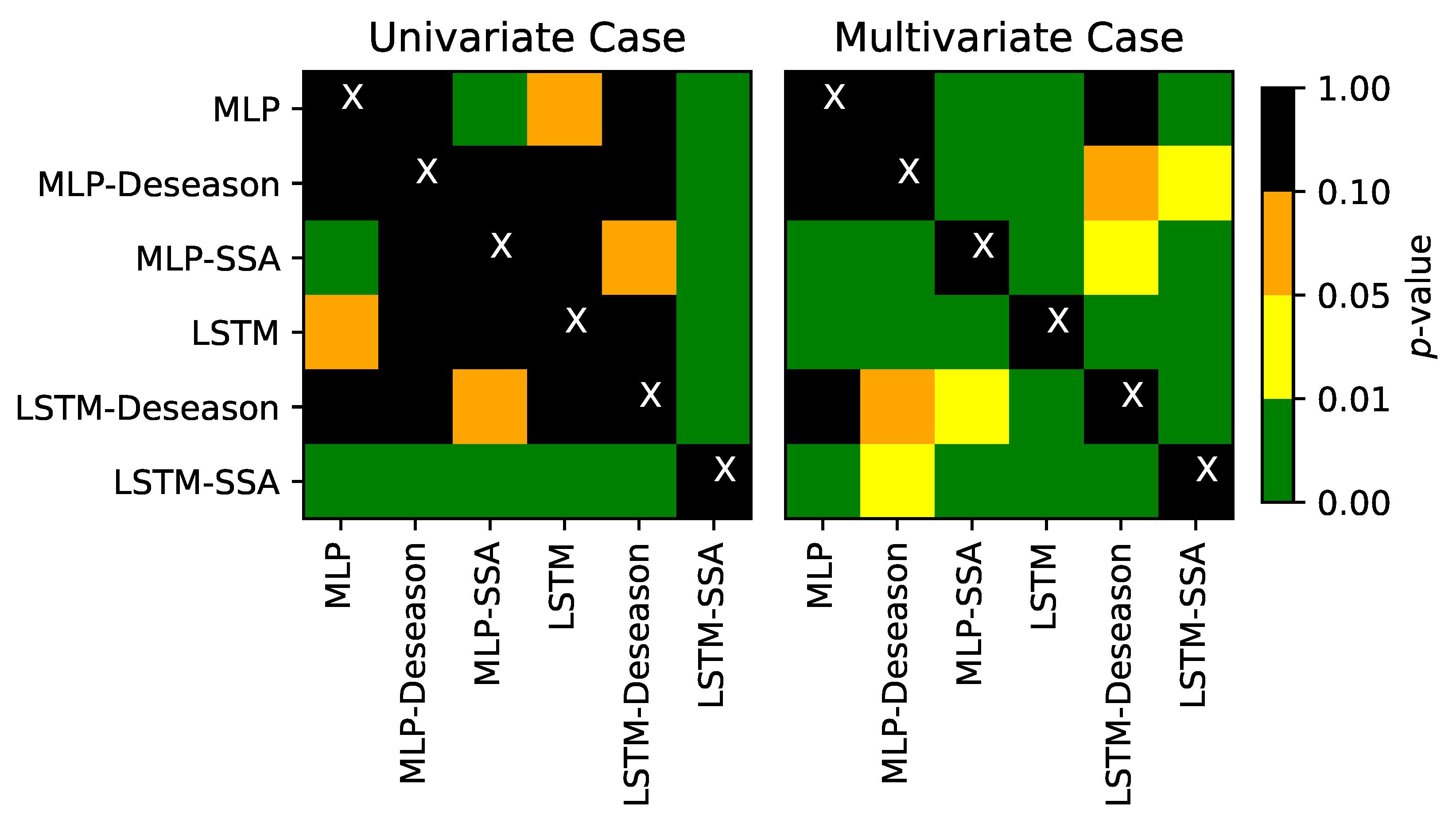
4.3. Assessing Statistical Significance

To validate the results, we performed pairwise DM tests to assess whether differences in model performance are statistically significant. We restricted this analysis only for the ANN-based models and presented the results for the Greek System Load dataset. Figure 6 presents the results in the form of a heatmap both for the univariate and multivariate cases for the Greek System Load. The key takeaway is that applying the SSA-based decomposition, prior to model training, leads to statistically significant improvement in forecast accuracy. This result holds true both for the MLP and the LSTM models, with the results being significant at the $1\%$ level. Similar results were observed for the GEFCom 2012 dataset.

5. Conclusions

In this work, we proposed a hybrid methodology to combine SSA-based decomposition with ANNs and, in particular LSTMs, for predicting day-ahead hourly electricity load. The proposed approach suggests decomposing the trajectory matrix via SVD and employing the extracted PCs, corresponding to trend, seasonal, and noise components, as exogenous regressors in a global ANN model.

Overall, the results on two real-world are consistent in showing that the decomposition step reduces the prediction error for both MLPs and LSTMs. This holds true when also accounting for the impact of exogenous features, such as weather forecasts, although the effect is less pronounced in that case. A notable result is that seasonal differentiation leads to diminished predictive performance against the general consensus that ANNs perform better when trained with seasonally adjusted time series [22]. It should be noted, however, that we consider a MIMO forecasting strategy while most of the literature regarding ANNs considers recursive forecasts. Future work will focus on quantifying the uncertainty in the predictions and on improving the proposed approach by testing additional ANN architectures and by refining the decomposition step.

References

1. Spodniak, P.; Ollikka, K.; Honkapuro, S. The impact of wind power and electricity demand on the relevance of different short-term electricity markets: The Nordic case. Appl. Energy 2021, 283, 116063. [Google Scholar] [CrossRef]
2. Goodarzi, S.; Perera, H.N.; Bunn, D. The impact of renewable energy forecast errors on imbalance volumes and electricity spot prices. Energy Policy 2019, 134, 110827. [Google Scholar] [CrossRef]
3. Hong, T.; Fan, S. Probabilistic electric load forecasting: A tutorial review. Int. J. Forecast. 2016, 32, 914–938. [Google Scholar] [CrossRef]
4. Box, G.E.; Jenkins, G.M.; Reinsel, G.C.; Ljung, G.M. Time Series Analysis: Forecasting and Control; John Wiley & Sons: Hoboken, NJ, USA, 2015. [Google Scholar]
5. Pappas, S.S.; Ekonomou, L.; Moussas, V.; Karampelas, P.; Katsikas, S. Adaptive load forecasting of the Hellenic electric grid. J. Zhejiang Univ. Sci. A 2008, 9, 1724–1730. [Google Scholar] [CrossRef]
6. Hippert, H.S.; Pedreira, C.E.; Souza, R.C. Neural networks for short-term load forecasting: A review and evaluation. IEEE Trans. Power Syst. 2001, 16, 44–55. [Google Scholar] [CrossRef]
7. Karampelas, P.; Vita, V.; Pavlatos, C.; Mladenov, V.; Ekonomou, L. Design of artificial neural network models for the prediction of the Hellenic energy consumption. In Proceedings of the 10th Symposium on Neural Network Applications in Electrical Engineering, Belgrade, Serbia, 23–25 September 2010; IEEE: New York, NY, USA, 2010; pp. 41–44. [Google Scholar]
8. Ekonomou, L.; Christodoulou, C.; Mladenov, V. A short-term load forecasting method using artificial neural networks and wavelet analysis. Int. J. Power Syst 2016, 1, 64–68. [Google Scholar]
9. Chen, B.J.; Chang, M.W. Load forecasting using support vector machines: A study on EUNITE competition 2001. IEEE Trans. Power Syst. 2004, 19, 1821–1830. [Google Scholar] [CrossRef] [Green Version]
10. Taylor, J.W.; McSharry, P.E. Short-term load forecasting methods: An evaluation based on european data. IEEE Trans. Power Syst. 2007, 22, 2213–2219. [Google Scholar] [CrossRef] [Green Version]
11. Papaioannou, G.; Dikaiakos, C.; Dramountanis, A.; Papaioannou, P. Analysis and modeling for short-to medium-term load forecasting using a hybrid manifold learning principal component model and comparison with classical statistical models (SARIMAX, Exponential Smoothing) and artificial intelligence models (ANN, SVM): The case of Greek electricity market. Energies 2016, 9, 635. [Google Scholar]
12. Kuo, P.H.; Huang, C.J. A high precision artificial neural networks model for short-term energy load forecasting. Energies 2018, 11, 213. [Google Scholar] [CrossRef] [Green Version]
13. Kiprijanovska, I.; Stankoski, S.; Ilievski, I.; Jovanovski, S.; Gams, M.; Gjoreski, H. Houseec: Day-ahead household electrical energy consumption forecasting using deep learning. Energies 2020, 13, 2672. [Google Scholar] [CrossRef]
14. Hochreiter, S.; Schmidhuber, J. Long short-term memory. Neural Comput. 1997, 9, 1735–1780. [Google Scholar] [CrossRef]
15. Bianchi, F.M.; Maiorino, E.; Kampffmeyer, M.C.; Rizzi, A.; Jenssen, R. Recurrent Neural Networks for Short-Term Load Forecasting: An Overview and Comparative Analysis; Springer: Berlin/Heidelberg, Germany, 2017. [Google Scholar]
16. Kong, W.; Dong, Z.Y.; Jia, Y.; Hill, D.J.; Xu, Y.; Zhang, Y. Short-term residential load forecasting based on LSTM recurrent neural network. IEEE Trans. Smart Grid 2017, 10, 841–851. [Google Scholar] [CrossRef]
17. Bouktif, S.; Fiaz, A.; Ouni, A.; Serhani, M.A. Single and multi-sequence deep learning models for short and medium term electric load forecasting. Energies 2019, 12, 149. [Google Scholar] [CrossRef] [Green Version]
18. Tian, C.; Ma, J.; Zhang, C.; Zhan, P. A deep neural network model for short-term load forecast based on long short-term memory network and convolutional neural network. Energies 2018, 11, 3493. [Google Scholar] [CrossRef] [Green Version]
19. He, W. Load forecasting via deep neural networks. Procedia Comput. Sci. 2017, 122, 308–314. [Google Scholar] [CrossRef]
20. Taylor, J.W. Short-term electricity demand forecasting using double seasonal exponential smoothing. J. Oper. Res. Soc. 2003, 54, 799–805. [Google Scholar] [CrossRef]
21. Hyndman, R.J.; Athanasopoulos, G. Forecasting: Principles and Practice; OTexts: Melbourne, Australia, 2018. [Google Scholar]
22. Zhang, G.P.; Qi, M. Neural network forecasting for seasonal and trend time series. Eur. J. Oper. Res. 2005, 160, 501–514. [Google Scholar] [CrossRef]
23. Taieb, S.B.; Bontempi, G.; Atiya, A.F.; Sorjamaa, A. A review and comparison of strategies for multi-step ahead time series forecasting based on the NN5 forecasting competition. Expert Syst. Appl. 2012, 39, 7067–7083. [Google Scholar] [CrossRef] [Green Version]
24. Cleveland, R.B.; Cleveland, W.S.; McRae, J.E.; Terpenning, I. STL: A seasonal-trend decomposition. J. Off. Stat. 1990, 6, 3–73. [Google Scholar]
25. De Livera, A.M.; Hyndman, R.J.; Snyder, R.D. Forecasting time series with complex seasonal patterns using exponential smoothing. J. Am. Stat. Assoc. 2011, 106, 1513–1527. [Google Scholar] [CrossRef] [Green Version]
26. Elsner, J.B.; Tsonis, A.A. Singular Spectrum Analysis: A New Tool in Time Series Analysis; Springer Science & Business Media: New York, NY, USA, 2013. [Google Scholar]
27. Bandara, K.; Bergmeir, C.; Hewamalage, H. LSTM-MSNet: Leveraging forecasts on sets of related time series with multiple seasonal patterns. IEEE Trans. Neural Netw. Learn. Syst. 2020, 32, 1586–1599. [Google Scholar] [CrossRef] [Green Version]
28. Wang, C.; Zhang, H.; Ma, P. Wind power forecasting based on singular spectrum analysis and a new hybrid Laguerre neural network. Appl. Energy 2020, 259, 114139. [Google Scholar] [CrossRef]
29. Moreno, S.R.; dos Santos Coelho, L. Wind speed forecasting approach based on singular spectrum analysis and adaptive neuro fuzzy inference system. Renew. Energy 2018, 126, 736–754. [Google Scholar] [CrossRef]
30. Liu, H.; Mi, X.; Li, Y.; Duan, Z.; Xu, Y. Smart wind speed deep learning based multi-step forecasting model using singular spectrum analysis, convolutional Gated Recurrent Unit network and Support Vector Regression. Renew. Energy 2019, 143, 842–854. [Google Scholar] [CrossRef]
31. Liu, H.; Mi, X.; Li, Y. Smart multi-step deep learning model for wind speed forecasting based on variational mode decomposition, singular spectrum analysis, LSTM network and ELM. Energy Convers. Manag. 2018, 159, 54–64. [Google Scholar] [CrossRef]
32. Moreno, S.R.; da Silva, R.G.; Mariani, V.C.; dos Santos Coelho, L. Multi-step wind speed forecasting based on hybrid multi-stage decomposition model and long short-term memory neural network. Energy Convers. Manag. 2020, 213, 112869. [Google Scholar] [CrossRef]
33. Hong, T.; Pinson, P.; Fan, S. Global energy forecasting competition 2012. 2014. Available online: https://doi.org/10.1016 (accessed on 20 May 2021).
34. Broomhead, D.S.; King, G.P. Extracting qualitative dynamics from experimental data. Phys. D Nonlinear Phenom. 1986, 20, 217–236. [Google Scholar] [CrossRef]
35. Takens, F. Detecting strange attractors in turbulence. In Dynamical Systems and Turbulence, Warwick 1980; Springer: Berlin/Heidelberg, Germany, 1981; pp. 366–381. [Google Scholar]
36. Golyandina, N.; Nekrutkin, V.; Zhigljavsky, A.A. Analysis of Time Series Structure: SSA and Related Techniques; Chapman and Hall/CRC: Boca Raton, FL, USA, 2001. [Google Scholar]
37. Graves, A.; Schmidhuber, J. Framewise phoneme classification with bidirectional LSTM and other neural network architectures. Neural Netw. 2005, 18, 602–610. [Google Scholar] [CrossRef] [PubMed]
38. Hong, T.; Wang, P.; White, L. Weather station selection for electric load forecasting. Int. J. Forecast. 2015, 31, 286–295. [Google Scholar] [CrossRef]
39. Wang, P.; Liu, B.; Hong, T. Electric load forecasting with recency effect: A big data approach. Int. J. Forecast. 2016, 32, 585–597. [Google Scholar] [CrossRef] [Green Version]
40. Bergstra, J.; Bengio, Y. Random search for hyper-parameter optimization. J. Mach. Learn. Res. 2012, 13, 281–305. [Google Scholar]
41. Chollet, F. Keras. 2015. Available online: https://github.com/fchollet/keras (accessed on 4 July 2021).
42. Hyndman, R.J.; Khandakar, Y. Automatic time series forecasting: The forecast package for R. J. Stat. Softw. 2008, 26, 1–22. [Google Scholar]
43. Diebold, F.X.; Mariano, R.S. Comparing predictive accuracy. J. Bus. Econ. Stat. 2002, 20, 134–144. [Google Scholar] [CrossRef]
Figure 1. Visualization of a basic LSTM cell architecture.
Energies 14 04107 g001
Figure 2. Flowchart for the multivariate case, showing a selection of PCs. The outcome of the dense layer is concatenated to the derived PCs, in the case exogenous data are included in the model.
Energies 14 04107 g002
Figure 3. Cumulative percentage of variance explained by the first 10 principal components for the Greek System Load.
Energies 14 04107 g003
Figure 4. Average daily profile in hourly resolution of load (blue) and standard deviation (shaded) of Greek System Load for one month of observations.
Energies 14 04107 g004
Figure 5. Scatterplot of Greek System Load vs. solar radiation (above) and temperature (below) for 12 pm.
Energies 14 04107 g005
Figure 6. Pairwise DM tests to assess if difference in performance is statistically significant for the univariate (left) and the multivariate (right) cases. The null hypothesis states that each pair of forecasts have the same predictive accuracy. Green, yellow, and orange denote that the null hypothesis is rejected and that the results are statistically significant at the 1 % ,   5 % , and 10 % levels, respectively. For p-value 0.10 , the null hypothesis is not rejected.
Energies 14 04107 g006