An Effective Acoustic Impedance Imaging Based on a Broadband Gaussian Beam Migration

Abstract

The estimation of the subsurface acoustic impedance (AI) model is an important step of seismic data processing for oil and gas exploration. The full waveform inversion (FWI) is a powerful way to invert the subsurface parameters with surface acquired seismic data. Nevertheless, the strong nonlinear relationship between the seismic data and the subsurface model will cause nonconvergence and unstable problems in practice. To divide the nonlinear inversion into some more linear steps, a 2D AI inversion imaging method is proposed to estimate the broadband AI model based on a broadband reflectivity. Firstly, a novel scheme based on Gaussian beam migration (GBM) is proposed to produce the point spread function (PSF) and conventional image of the subsurface. Then, the broadband reflectivity can be obtained by implementing deconvolution on the image with respect to the calculated PSF. Assuming that the low-wavenumber part of the AI model can be deduced by the background velocity, we implemented the AI inversion imaging scheme by merging the obtained broadband reflectivity as the high-wavenumber part of the AI model and produced a broadband AI result. The developed broadband migration based on GBM as the computational hotspot of the proposed 2D AI inversion imaging includes only two GBM and one Gaussian beam demigraton (Born modeling) processes. Hence, the developed broadband GBM is more efficient than the broadband imaging using the least-squares migrations (LSMs) that require multiple iterations (every iteration includes one Born modeling and one migration process) to minimize the objective function of data residuals. Numerical examples of both synthetic data and field data have demonstrated the validity and application potential of the proposed method.

1. Introduction

As the consumption of oil and gas resources increases, the target of seismic exploration is shifting from the large-scale structural reservoirs to small-scale stratigraphic reservoirs [1]. Acoustic impedance (AI), as a basic physical parameter, is defined as the product of density and velocity, which plays a key role to connect the surface seismic data to the subsurface model [2,3]. Therefore, the broadband AI imaging is crucial for seismic interpretation and beneficial to reservoir predication [4,5].

The typical method of AI estimation is to obtain the subsurface reflectivity first and then to calculate the AI. A recursive formula expressed by the reflectivity of normal incident is commonly used for AI estimation [6,7], followed by a prepared reflectivity from the conventional seismic migration. However, the recursive algorithm is sensitive to noise and often causes accumulated errors and inversion instabilities [8]. Furthermore, the recursive algorithm is usually applied to 1D seismic traces, but the spatial coherence of the subsurface model cannot be incorporated into the AI inversion [9,10]. To overcome the limitations of the 1D AI inversion, the full waveform inversion (FWI) [11,12,13] has been developed to estimate the broadband velocity of AI model in 2D and 3D cases. However, the strong nonliner relationship between the seismic data and the subsurface model will cause nonconvergence and unstable problems in practice.

The travel time-based velocity tomography and the conventional migrations are widely used linear inversion methods [14,15], and the full subsurface AI model can also be divided into two parts, the low-wavenumber, and the high-wavenumber parts, for two different linear inversion methods, respectively [16]. The low-wavenumber part is the background model, which can be obtained by tomography [17]. The subsurface reflectivity is related to the high-wavenumber part of AI, which can be inverted by seismic migrations [18]. The merging of the estimated low-wavenumber part and the high-wavenumber part of the AI model often leads to an intermediate wavenumber gap, and the intermediate wavenumber components are usually poorly reconstructed [14]. In recent years, the broadband, wide-azimuth, and high-density seismic data acquisition technologies have been proposed for broadband and true-amplitude seismic imaging [1,19], offering possibilities to bridge the intermediate wavenumber gap.

The least-squares migration (LSM) is a powerful method for seismic imaging of the broadband reflectivity [20,21,22]. Different LSM imaging schemes can be developed based on different seismic wave propagators. The ray-based Kirchhoff migrations method [23,24] performs efficiently but suffers accuracy problems in areas with complex subsurface. The two-way wave-based least-squares reverse time migration (LSRTM) is known as the most accurate imaging method. However, it is also known as the most expensive LSM for computation cost [25,26]. Gaussian beam is a one-way wave propagator that inherits the flexibility of ray and the accuracy of wave equation, and which has an extensive application in seismic modeling and migration [27,28,29,30,31,32]. Gaussian beam migration (GBM) can be extended for LSM by minimizing the objective function of residuals between the simulated data and the observed data [33,34]. However, the iterative fitting in data domain is a computationally intensive job, usually requiring more than 10 iterations for an acceptable result [35]. There are several noniterative approaches toward the similar goal of LSM by approximating the Hessian matrix and calculating its inverse matrix. Illumination effects linked with Hessian Matrix have been proved to be very important in retrieving the broadband reflectivity [36,37]. From the perspective of illumination analysis, the noniterative broadband reflectivity imaging can employ Kirchhoff migrations [38,39], finite difference (FD) migrations [40,41] and beam-based migrations [19]. The point spread function (PSF), as the localized elements of the full Hessian matrix, can be linked to the illumination [42,43] and produce a broadband reflectivity by a PSF-based deconvolution [44].

In this paper, we propose an effective AI imaging approach based on a broadband reflectivity imaging profile under the assumption that the background velocity or AI has been obtained by tomography. Firstly, we adopted GBM to implement migration process and calculated the PSF with the prepared background velocity. Then, we used the PSFs to deconvolve the image of GBM to produce a broadband subsurface reflectivity as the high-wavenumber part of AI model. Finally, we implemented the full AI inversion imaging by merging the obtained broadband reflectivity and the low-wavenumber part of AI model that can be derived from background velocity under assumption of constant density.

2. The Principle of Gaussian Beam Migration

Gaussian beam is an asymptotic solution of wave equation in a coordinate system centered on a ray under the high-frequency approximation, which combines the merits of both wave equation and ray theory. The frequency domain solution [28] of the Gaussian beam of a scalar wave equation can be expressed as

$$u_{\mathrm{GB}}(s,q_1,q_2,\omega )=\sqrt{\frac{v(s)\det Q(s_0)}{v(s_0)\det Q(s)}}\exp \left\{i\omega \left[\tau (s)+\frac{1}{2}{\mathit{q}}^T[P(s)Q^{-1}(s)]\mathit{q}\right]\right\}$$

(1)

where $s$ and ${\mathit{q}}^T=(q_1,q_2)$ refer to the coordinates along and perpendicular to the centered-ray in the ray-centered coordinates, $w$ is the circular frequency and $s_0$ is the initial point of ray. The real functions $v(s)$ and $\tau (s)$ refer to velocity and travel time along the path of centered-ray, respectively, which can be computed by kinematic ray tracing. The complex functions $P(s)$ and $Q(s)$ refer to the dynamic ray parameters, which can be computed by dynamic ray tracing. For GBM, the Green’s function can be decomposed into a summation of Gaussian beams [29,45]

$$G(x, x_s, \omega )\approx \frac{i\omega }{2\pi }{\displaystyle \iint \frac{d{p}_x^{s}d{p}_y^s}{p_z^s}}{u}_{GB}(x, x_s, p_{}^s, \omega )$$

(2)

where $u_{GB}$ is an individual Gaussian beam in Cartesian coordinates, $\mathit{x}$ refers to the coordinate of subsurface space, ${\mathit{x}}_s$ refers to the location of the source on the surface and $p_{}^s=(p_x^s, p_y^s, p_z^s)$ refers to the slowness vector in the initial emergence direction of the local plane-wave. For implementing the pre-stack GBM, we use the classic imaging condition of cross-correlation as below:

$$I(x)=\frac{-1}{2\pi }{\displaystyle \int d\omega }{\displaystyle \int d{x}_r}{\displaystyle \int d{x}_s}\frac{\partial G^{\ast }(x,x_r,\omega )}{\partial z_r}G(x,x_s,\omega )D(x_{\mathrm{r}},x_{\mathrm{s}},\omega )$$

(3)

where $G(x,x_s,\omega )$ is the background Green’s function with the source, and $G^{*}(x,x_r,\omega )$ is the conjugate of background Green’s functions with the receiver. Both can be calculated using Equation (2), describing wave propagation from source and receiver locations to the image point, respectively. $D(x_r,x_s,\omega )$ is the recorded pre-stack data in frequency domain, and $x_r$ represents the coordinate of the receiver.

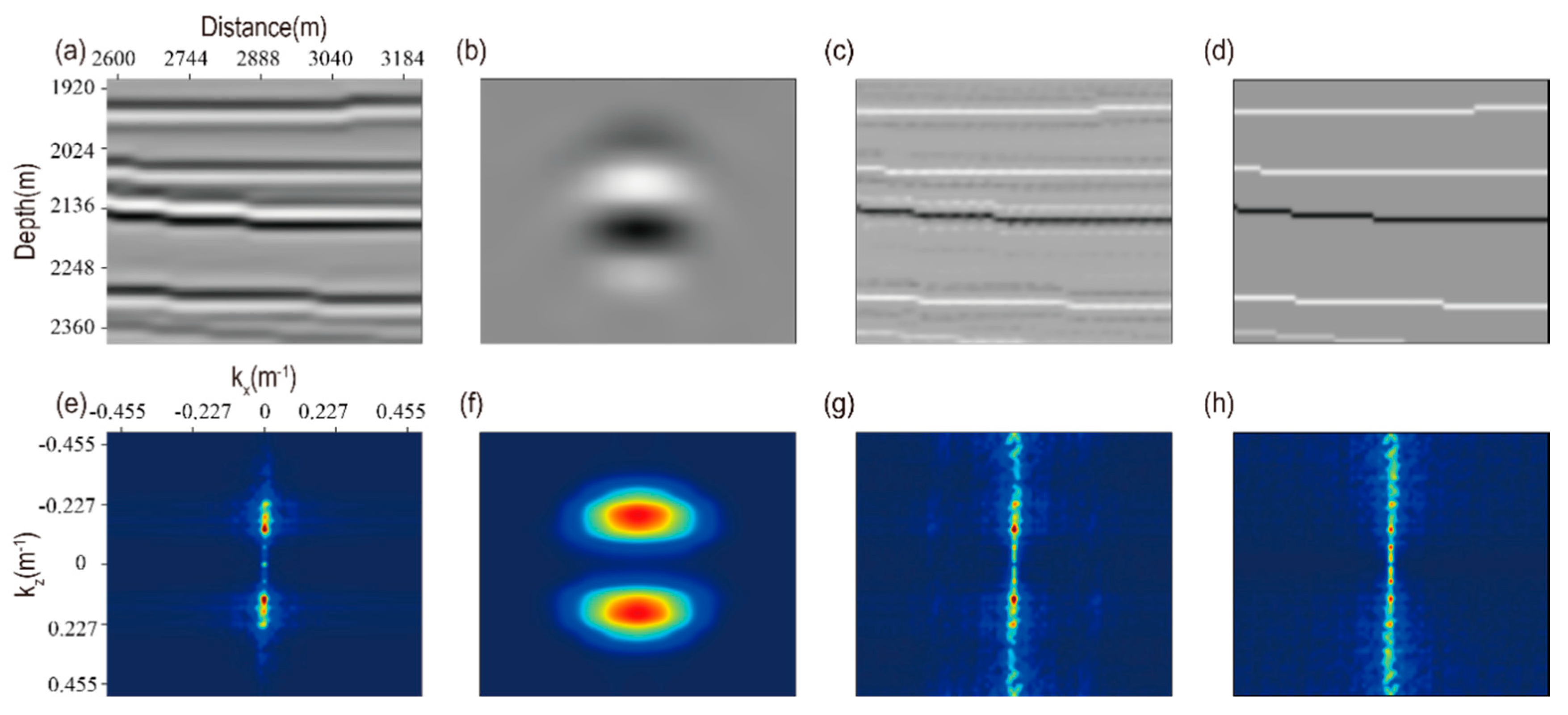
3. The Broadband Reflectivity Estimation Based on Point Spread Function

The pre-stack GBM image calculated using Equation (3) can be related to the subsurface reflectivity through a PSF in the local wavenumber domain [42]

$$I(x, k)=P(x, k)R(x, k)$$

(4)

where $k$ refers to the local wavenumber, $I(x, k)$ refers to the imaging result of conventional migration, $P(x, k)$ presents the PSF and $R(x, k)$ refers to the reflectivity of subsurface model. All quantities in Equation (4) are dual domain functions, which are in local wavenumber domain defined in a small area adjacent to $x$. We see that the PSF serves as a filter that blurs the reflectivity and converts it into a distorted image. If the localized PSF is available, the conventional imaging result can be corrected to recover the reflectivity, as below:

$$R_{\mathrm{c}}(x, k)=\frac{I(x, k)}{P(x, k)}$$

(5)

where $R_c$ refers to the obtained broadband image after correction. The calculation of PSF, a localized expression the full Hessian matrix $P(x, k)$, is the key step of broadband reflectivity estimation.

In this study, a novel scheme for PSF calculating the PSF by using the GBM is developed based on the method of Chen and Xie [46] and Kang et al. [47]. Note that Equation (4) is a multiplication operation in the local wavenumber domain, which is equivalent to convolution operation in the spatial domain.

$$I(x, x_k)=P(x, x_k)\ast R(x, x_k)$$

(6)

where, the local coordinate $x_k$ refers to the inverse FFT of local wavenumber $k$. The PSF $P(x, x_k)$ equals to the conventional imaging result $I(x, x_k)$ if the reflectivity model is replaced by a model with scatters (every single scatter presents a delta function in mathematical aspect). From the perspective of seismic migration, the PSF $P(x, x_k)$ can be obtained straightforward by imaging the seismic scattering wave of the scatter-point model. The Born modeling [48] is generated on the scatter-point model to simulate the original pre-stack data:

$$D_s(x_{\mathrm{r}}, x_s, \omega )=2{\omega }^2{\displaystyle {\int }_{D}G(x, x_s, \omega )m_s\left(x\right)G(x, x_r, \omega )\mathrm{d}x}$$

(7)

where $D_s$ is the simulated data, and $m_s(x)$ is scatter-point model, which includes many scatter points (perturbation of delta functions) embedded into the background model. If the Green’s functions of Gaussian beam Equation (2) are prepared, we can obtain the pre-stack data $D_s$ by the integration of Equation (7). Then, we can calculate the PSF $P(x, x_k)$ in space domain by applying $D_s$ to Equation (3). In order to correct the image in wavenumber domain, the local FFT and the inverse FFT are generated before and after correction, and a stable factor is applied to the denominator of Equation (5) for a stabilized division.

Since the PSF includes all illumination and resolution effects from the acquisition layout, the geologic structure of subsurface and seismic wavelet, etc., and the division operation in Equation (5) tend to reverse those effects. From the prospective of LSM, the inverse of PSF can not only recover the imaging amplitude for subsurface structures but also brings a deblurring effect to the image to enhance its resolution, achieving a broadband imaging result.

4. The Impedance Inversion Based on the Estimated Reflectivity

The reflectivity of normal incidence is the high-wavenumber part of AI, which is important for seismic interpretation [49,50]. The 1D reflectivity of normal incidence can be expressed by AI as

$$r_i=\frac{{\rho }_{i+1}{v}_{i+1}-{\rho }_i{v}_i}{{\rho }_{i+1}{v}_{i+1}+{\rho }_i{v}_i}=\frac{Z_{i+1}-Z_i}{Z_{i+1}+Z_i}$$

(8)

where ${\rho }_{i+1}, v_{i+1} and Z_{i+1}={\rho }_{i+1}{v}_{i+1}$ are density, velocity and AI in the ${(i+1)}^{th}$ layer, respectively, and $r_i, {\rho }_i, v_i and Z_i={\rho }_i{v}_i$ are reflectivity, density, velocity and AI in the $i^{th}$ layer, respectively. If the absolute value of the reflection coefficients is small, this nonlinear relationship between the reflectivity and the AI can be reformulated according to [51]:

$$r_i=\frac{\ln Z_{i+1}-\ln Z_i}{2}$$

(9)

We adopt $a=(\ln Z)/2$, and the liner relationship between 1D reflectivity and $a$ can be derived by

$$r={\nabla }_{z}a$$

(10)

where, $r$ refers to the 1D reflection coefficients series of all reflectors and $a$ refers to the corresponding series of half natural log of AI. ${\nabla }_z$ refers to vertical one-order difference operator.

By considering the spatial coherence between traces of the AI model, we incorporate the 2D seismic profiles and employ the forward model that solves for multitraces simultaneously. Equation (10) can be extended to the 2D case according to [9]:

$$R={\nabla }_{n}A$$

(11)

where $R=\left(r_1,r_2,\dots ,r_M\right)$ refers to a matrix that denotes the reflectivity imaging profile of normal incidence, the matrix $A=\left(a_1,a_2,\dots ,a_M\right)$ denotes the corresponding profile of half natural log of AI and ${\nabla }_n$ refers to vertical one-order difference operator in the normal direction of the reflector. The TV regularization is introduced to preserve the blocky characteristics of structure, and the AI profile can be estimated as follows [9]:

$$\arg \underset{A}{\min }{\Vert A\Vert }_{T{V}_{}} subject to \{\begin{array}{l}{\Vert {\nabla }_{n}A-R\Vert }_2^2<\epsilon \\ A_{low}=LA\end{array}$$

(12)

Here, $A_{low}$ is the given background of $A$, and $L$ refers to the low-pass filter. $A_{low}=LA$ is a boundary constraint condition in this AI inversion scheme. In this scheme, the broadband reflectivity takes the role of seaming the wavenumber gap between the low-wavenumber part of AI and the high-wavenumber part. In the case of 2D model, the TV norm in Equation (12) can be written as

$${\Vert A\Vert }_{TV}={\displaystyle \iint \sqrt{{\left({\nabla }_{x}A\right)}^2+{\left({\nabla }_{z}A\right)}^2}}dxdz$$

(13)

where ${\nabla }_x$ is the horizontal one-order difference operator. The constrained inversion problem Equation (12) cannot be solved directly, as the TV regularization term is nondifferentiable. The Bregman iteration inversion method [52] and the Shrinkage–Thresholding method [53] can be introduced to solve this problem.

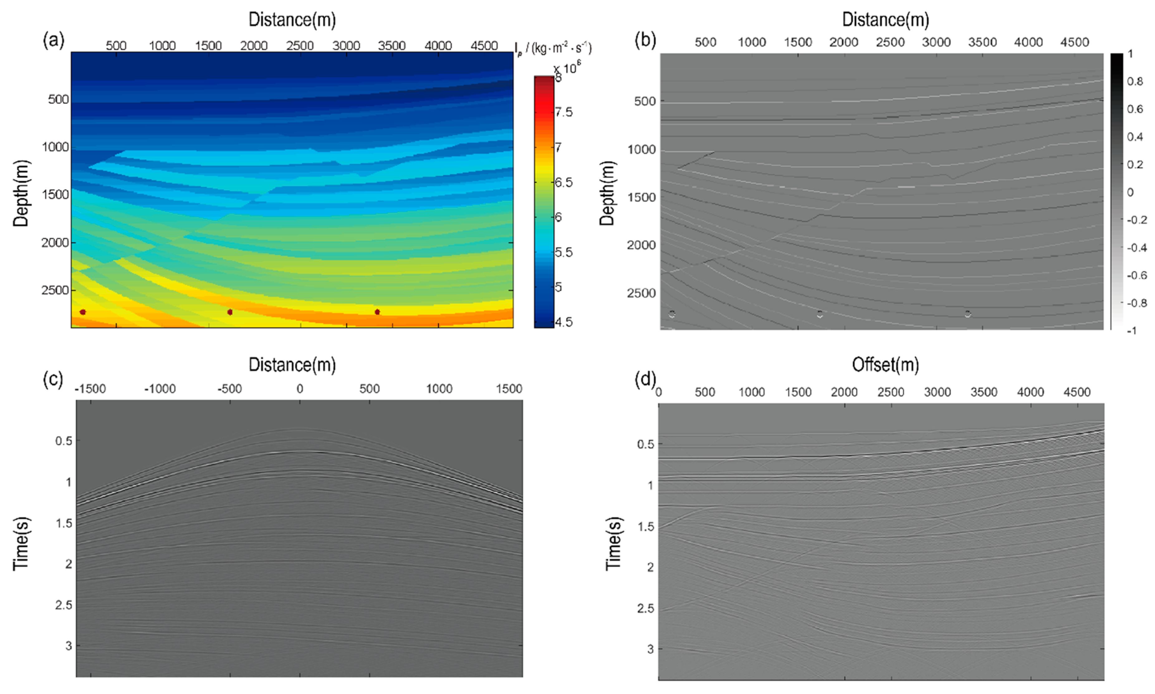
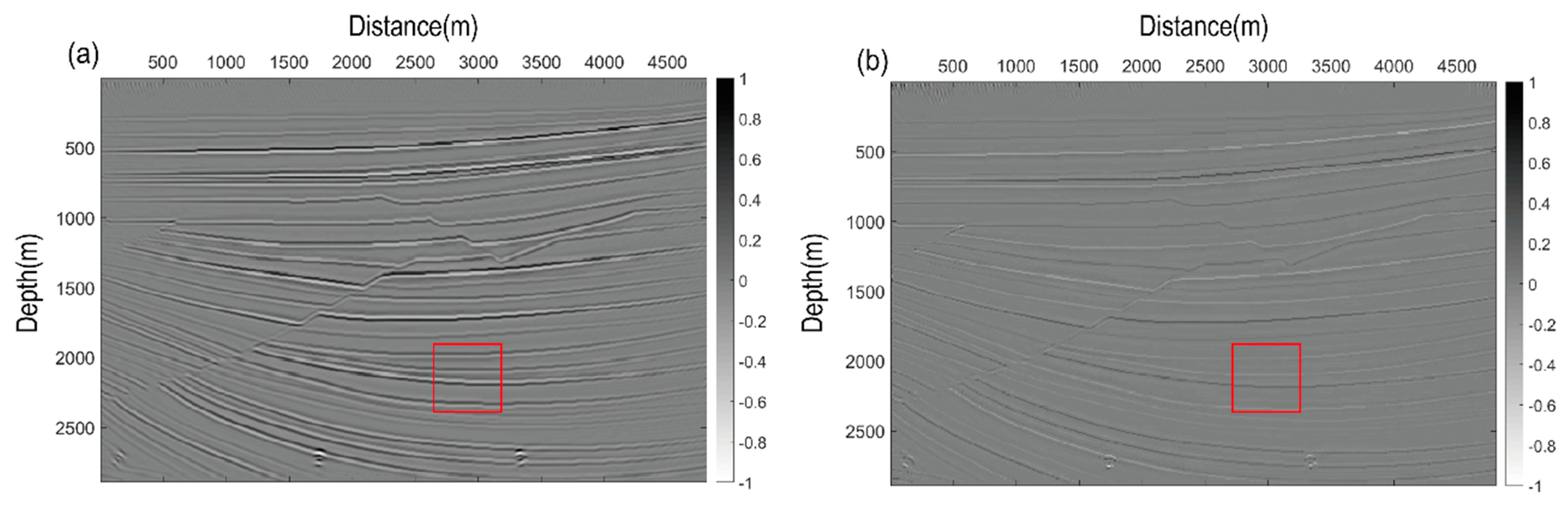
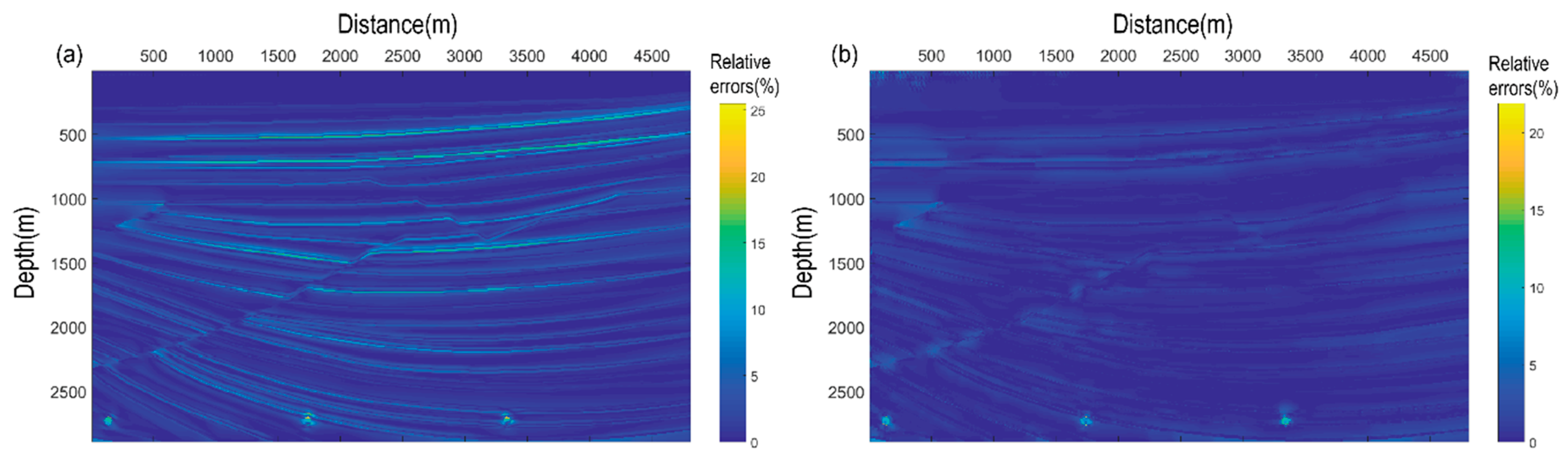
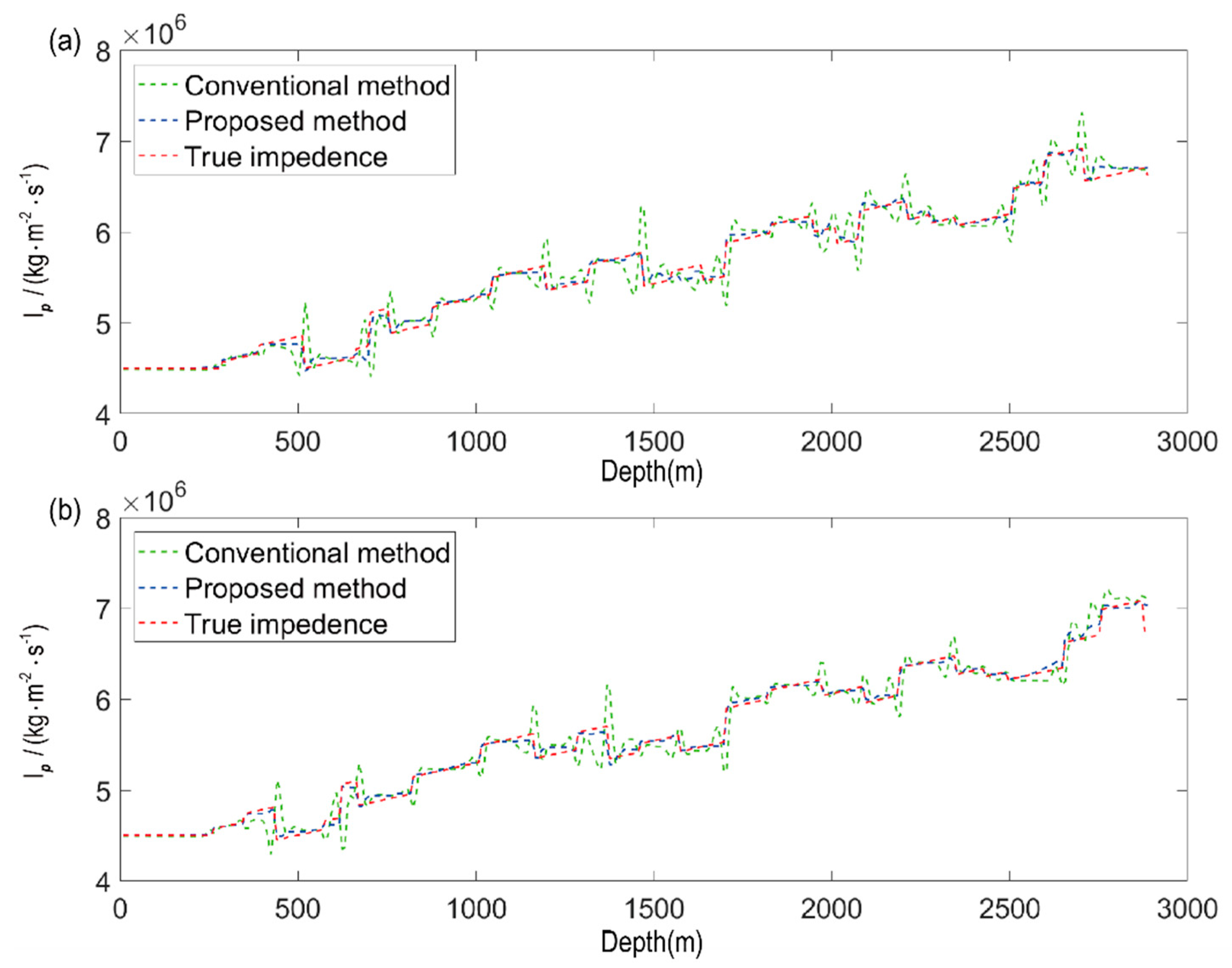
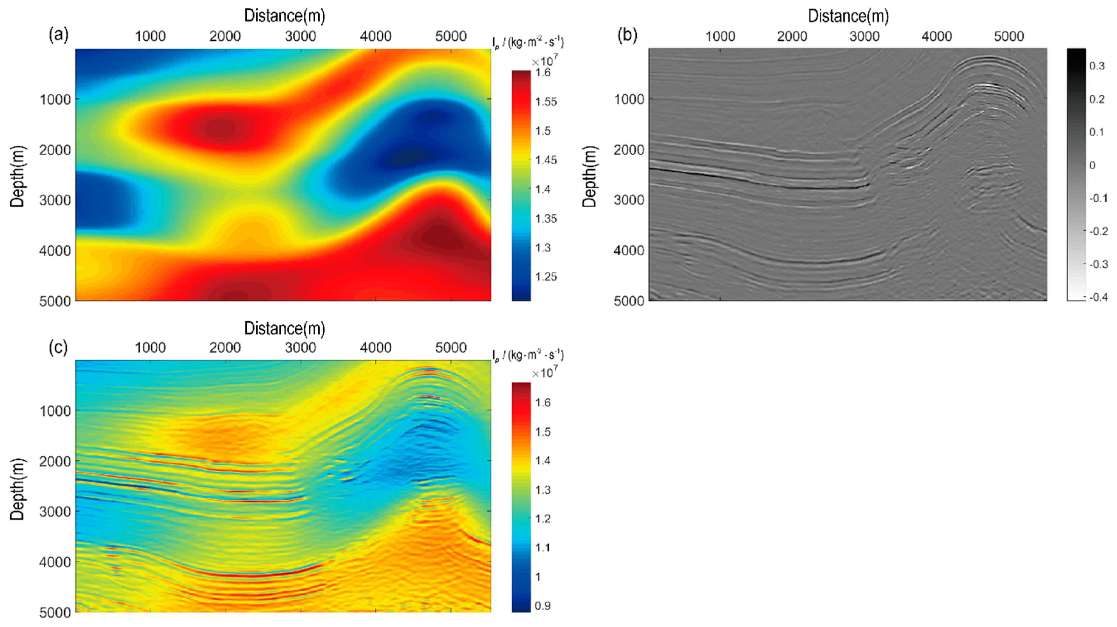
5. Numerical Examples

The Sigsbee2a model was designed according to the geological background near the Sigsbee escarpment, containing several normal and thrust faults that separate the sedimentary deposits [54]. The left part of the Sigsbee2a model was chosen to test the proposed method, which is parameterized by 361 × 601 mesh points in the 2D model and 8 m sampling intervals in both horizontal and vertical directions. The true impedance and reflectivity model are shown in Figure 1a,b, respectively. The FD-based Born modeling was used for the original pre-stack data, and a Ricker wavelet with the main spectrum in 25 Hz was selected for the modeling. The pre-stack data set contains 150 shots that are evenly distributed on the surface with a 32 m sampling interval. Each common shot point gathered has 201 receivers arrayed with offset from −1600 m to 1600 m at a 16 m spacing. A sorted common shot gather that is located at 2880 m, and the zero offset gather are shown in Figure 1c,d, respectively.

To produce the PSFs for correction, we inserted 493 point scatterers in the background (migration) velocity with a 168 m sampling interval in both horizontal and vertical directions. The pre-stack diffracted data can be generated by using the Born modeling method on the designed point scatterers model, as calculated by Equation (7). Based on the obtained diffracted data in Equation (7), we implemented the conventional GBM to produce all subsurface PSFs at once. The PSFs in space domain are shown in Figure 2a, which contain the main blurring effects of the conventional migration as a localized Hessian matrix of the inversion imaging system. One PSF in Figure 2a is zoomed in to show its shape in details, but it still has not directly revealed seismic illumination. Therefore, we implemented the FFT to obtain the spectrum of the PSFs in local wavenumber domain, which are illustrated in Figure 2b. In addition to illuminating all PSFs in the whole model, we also zoomed out one PSF to show its spectrum in detail, as the red rectangle shows in Figure 2b. We found that the PSFs in shallower positions have superior amplitude than the deeper ones, and the PSFs in the middle have broader wavenumber coverage than the sider ones, which reveals that the shallower and middle positions have better seismic illumination and coverage.

Next, we implemented conventional GBM to produce the subsurface image and then performed the correction to produce a broadband reflectivity using Equation (5). The image from the conventional GBM and the corrected image using the proposed method are shown in Figure 3a,b, respectively. By comparing conventional GBM image with the corrected reflectivity image, we found that the image after correction has more balanced amplitudes in both the shallower and the deeper parts of the model, as well as more abundant wavenumber contents. We chose a local part of the model to show the quantitative improvement of the PSF based correction. Figure 4a is the sorted local imaging result of conventional GBM, and Figure 4b–d are the corresponding PSF, local-corrected imaging result and the true reflectivity. Figure 4e–h are the spectrum of Figure 4a–d in local wavenumber domain. The results indicate that the spectrum of the corrected image has been recovered greatly, and it is very close to the true spectrum.

Owing to the broadband reflectivity that was obtained beforehand, the absolute AI imaging by using the boundary constraint inversion scheme can be implemented as Equation (12). The constant density of 2500 kg/m³ is used in this inversion scheme as Equation (12), and the low wavenumber part of AI is deduced by the background migration velocity. As shown in Figure 5a,b for comparison, we implemented this scheme by using conventional GBM image and the corrected image with PSF, respectively. By comparing the absolute AI results from the corrected image and the conventional GBM image, the AI inversed by the corrected image shows better consistency with the true AI model of Figure 1a. For further comparison between the inversed AI results from conventional GBM and the proposed method, we implemented the FFT to local areas of both results. Figure 5c,d show the spectrum of the areas marked by red rectangles; Figure 5e shows the spectrum of the corresponding true AI model in Figure 1a. We can see that the inverted impedance of the proposed method has a wider spectral band than the conventional one, and it has similar spectral pattern to the true spectrum. For quantitative comparison of the results in space domain, we measured the relative errors of the inverted AI profiles from both conventional GBM and the proposed broadband GBM. The comparison results in Figure 6a,b show that the relative errors of the proposed method are almost all below 5%, and the relative errors of traditional method are greater than 10% in many places. For further comparison of absolute value of the inverted AI, we extract two traces at 1840 m and 3280 m from Figure 5a,b, and the extracted traces are indicated in Figure 7a,b, respectively. The green, blue and red dashed lines represent the inverted impedance results from the conventional GBM, the proposed method and true reflectivity, respectively. It is obvious that the AI inversed by the proposed method is very close to the true AI, and the AI inversed by conventional GBM is far away from the true AI.

To further certify the application potential of this method, we also chose a field seismic data set for testing. The whole field data came from China, and we sorted 91 shots for testing. All sorted shots are located on the surface from 0 to 5500 m with a 60 m interval, and each shot has 75 receivers bilaterally located from offset 40 m to 3000 m at a spacing of 40 m. Figure 8a shows the background AI model from the industry, which is obtained by velocity analysis and tomography module of commercial software. Figure 8b shows the broadband reflectivity of the field data deduced by the proposed GBM. Figure 8c is the inverted AI through merging the obtained broadband reflectivity and background AI model. It can be found in Figure 8c that the detailed structural features of the inverted AI are consistent with the reflectivity profile of Figure 8b, and the macro features are consistent with the background AI of Figure 8a. This test demonstrates that the proposed AI inversion imaging scheme has the capability to merge the obtained broadband reflectivity and the given background AI and produce the absolute broadband AI model effectively.

6. Discussions

Today, the wide-azimuth and high-fidelity seismic datasets enable the high dimensional inversion imaging to estimate the subsurface parameters with higher resolution. The classic FWI is a popular high dimensional nonlinear inversion method from seismic data to subsurface model but usually suffers the “cycle-skipping” problem [55]. In this study, we focused on the broadband reflectivity under the linear LSM inversion frame and then estimated the broadband AI model by incorporating the background AI model. In other words, we divided the full model into different parts and tried to invert different parts by the linear inversion separately.

We developed the GBM to implement the LSM, because the GBM has better implementation efficiency and superiority for broadband imaging than the FD-based migrations. Specifically, the computational cost increased nearly 1600% when FD-based methods are used to propagate seismic wave with frequency from 30 Hz to 70 Hz, while beam-based method only requires less than a 90% increment in the same case [19]. Moreover, the GBM is a one-way propagator that does not have a back-scattering wave in propagation, and the GBM-based method has no problem of crosstalk noises in PSF calculation due to interferometry of scatter-points [46,55].

In this study, the low-wavenumber part of the model is assumed to be known beforehand, because this part is commonly inverted by travel time inversion [56], which is linear inversion and demonstrates higher stability than FWI. We used the constant density model in all the tests in this paper, because density is not sensitive to travel time, and it always couples with velocity in AI inversion. Although the acoustic wave equation with constant density is commonly used in the industry for impedance inversion as the geometric position of subsurface reflectors can be inverted without density [10,16,57], we are still in the transition from AI inversion to the elastic impedance inversion. Since well-logging is an effective way to get the density directly, the elastic impedance inversion can be developed to adapt spatial-variable density model in our future work.

7. Conclusions

As an alternative of the nonlinear inversion imaging, we propose an effective AI inversion imaging method based on a broadband GBM imaging. The extended GBM method is a linear imaging under LSM framework, which produces the broadband reflectivity as the high-wavenumber part of the AI model. The numerical tests demonstrate that the bandwidth of the reflectivity is important for inverting the detailed texture of the AI model, and the background AI should be included to guarantee the correct value of the absolute AI model.

The proposed broadband imaging method includes only one Gaussian beam Born modeling and two GBM processes, which is more efficient than the conventional LSM that requires multiple iterations of Born modeling and gradient calculation (migration). Benefitting from the implementation flexibility of beam-based method with complex geometry, this new method can be developed to process the AI inversion in the case of rugged topography straightforward. In addition, the developed method can be extended to 3D cases with less computational cost by using GBM than FD-based migrations.

References

1. Wang, H.Z.; Guo, S.; Zhou, Y. Broadband Acoustic Impedance Model Building for Broadband, Wide-Azimuth, and High-Density Seismic Data. Geophys. Pros. Pet. 2019, 58, 1–8. [Google Scholar]
2. Mabrouk, W.M. Acoustic Impedance Inversion Approach from Petrophysical Data. J. Pet. Sci. Eng. 2010, 73, 181–184. [Google Scholar] [CrossRef]
3. Alves, F.; Almeida, J.A.; Silva, A.P. Simulation of acoustic impedance images by stochastic inversion of post-stack seismic reflection amplitudes and well data. J. Pet. Sci. Eng. 2014, 121, 52–65. [Google Scholar] [CrossRef]
4. Zahmatkesh, I.; Kadkhodaie, A.; Soleimani, B.; Golalzadeh, A.; Azarpour, M. Estimating Vsand and Reservoir Properties from Seismic Attributes and Acoustic Impedance Inversion: A Case Study from the Mansuri Oilfield, SW Iran. J. Pet. Sci. Eng. 2018, 161, 259–274. [Google Scholar] [CrossRef]
5. Wu, H.; Chen, Y.P.; Li, S.; Peng, Z.M. Acoustic Impedance Inversion Using Gaussian Metropolis–Hastings Sampling with Data Driving. Energies 2019, 12, 2744. [Google Scholar] [CrossRef] [Green Version]
6. Walker, C.; Ulrych, T.J. Autoregressive Recovery of the Acoustic Impedance. Geophysics 1983, 48, 1338–1350. [Google Scholar] [CrossRef]
7. Oldenburg, D.W.; Scheuer, T.; Levy, S. Recovery of the Acoustic Impedance from Reflection Seismograms. Geophysics 1983, 48, 1318–1337. [Google Scholar] [CrossRef]
8. Berteussen, K.A.; Ursin, B. Approximate Computation of the Acoustic Impedance from Seismic Data. Geophysics 1983, 48, 1351–1358. [Google Scholar] [CrossRef]
9. Gholami, A. Nonlinear Multichannel Impedance Inversion by Total-Variation Regularization. Geophysics 2015, 80, R217–R224. [Google Scholar] [CrossRef]
10. Gholami, A. A Fast Automatic Multichannel Blind Seismic Inversion for High-Resolution Impe Dance Recovery. Geophysics 2016, 81, V357–V364. [Google Scholar] [CrossRef]
11. Tarantola, A. Inversion of Seismic Reflection Data in the Acoustic Approximation. Geophysics 1984, 49, 1259–1266. [Google Scholar] [CrossRef]
12. Lambaré, G.; Virieux, J.; Madariaga, R.; Jin, S. Iterative Asymptotic Inversion in the Acoustic Approximation. Geophysics 1992, 57, 1138–1154. [Google Scholar] [CrossRef]
13. Pratt, R.G. Seismic Waveform Inversion in the Frequency Domain, Part 1: Theory and Verify Cation in a Physical Scale Model. Geophysics 1999, 64, 888–901. [Google Scholar] [CrossRef] [Green Version]
14. Claerbout, J.F. Imaging the Earth's Interior; Blackwell Scientific Publications: Oxford, UK, 1985. [Google Scholar]
15. Wang, Y.; Pratt, R.G. Sensitivities of Seismic Traveltimes and Amplitudes in Reflection Tomography. Geophys. J. Int. 1997, 131, 618–642. [Google Scholar] [CrossRef] [Green Version]
16. Guo, S.; Wang, H. Seismic Absolute Acoustic Impedance Inversion with L1 Norm Reflectivity Constraint and Combined First- and Second-Order Total Variation Regularizations. J. Geophys. Eng. 2019, 16, 773–788. [Google Scholar] [CrossRef]
17. Feng, B.; Xu, W.; Wu, R.S.; Xie, X.B.; Wang, H. Finite-Frequency Traveltime Tomography Using the Generalized Rytov Approximation. Geophys. J. Int. 2020, 221, 1412–1426. [Google Scholar] [CrossRef]
18. Virieux, J.; Asnaashari, A.; Brossier, R.; Métivier, L.; Ribodetti, A.; Zhou, W. An Introduction to Full Waveform Inversion. In Encyclopedia of Exploration Geophysics; Society of Exploration Geophysicists: Tulsa, OK, USA, 2014; pp. R1-1–R1-40. [Google Scholar] [CrossRef]
19. Liu, S.Y.; Wu, R.S.; Feng, B.; Wang, H.Z.; Guo, S. A True-Amplitude Imaging Method Based on Gaussian Beam Migration and Demigration. P. Appl. Geophys. 2020, 177, 4707–4718. [Google Scholar] [CrossRef]
20. Beylkin, G. Imaging of Discontinuities in the Inverse Scattering Problem by Inversion of a Generalized Radon Transform. J. Mathe. Phys. 1985, 26, 99–108. [Google Scholar] [CrossRef]
21. Bleistein, N. On the Imaging of Reflectors in the Earth. Geophysics 1987, 52, 931–942. [Google Scholar] [CrossRef]
22. Bleistein, N.; Zhang, Y.; Xu, S.; Zhang, G.; Gray, S.H. Migration/Inversion: Think Image Point Coordinates, Process in Acquisition Surface Coordinates. Inverse Problems 2005, 21, 1715–1744. [Google Scholar] [CrossRef] [Green Version]
23. Nemeth, T.; Wu, C.; Schuster, G.T. Least-Squares Migration of Incomplete Reflection Data. Geophysics 1999, 64, 208–221. [Google Scholar] [CrossRef]
24. Duquet, B.; Marfurt, K.J.; Dellinger, K.J. Kirchhoff Modeling, Inversion for Reflectivity, and Subsurface Illumination. Geophysics 2000, 65, 1195–1209. [Google Scholar] [CrossRef]
25. Dai, W.; Huang, Y.; Schuster, G.T. Least-Squares Reverse Time Migration of Marine Data with Frequency-Selection Encoding. Geophysics 2013, 78, S233–S242. [Google Scholar] [CrossRef] [Green Version]
26. Ma, C.; Gao, Y.; Lu, C. Numerical Modeling of Elastic Wave in Frequency-Domain by Using Staggered Grid Fourth-Order Finite-Difference Scheme. Adv. Geo Energy Res. 2019, 3, 410–420. [Google Scholar] [CrossRef] [Green Version]
27. Cerveny, V.; Popov, M.M.; Psencik, I. Computation of Wave Fields in Inhomogeneous Media—Gaussian Beam Approach. Geophys. J. Int. 1982, 70, 109–128. [Google Scholar] [CrossRef] [Green Version]
28. Hill, N.R. Gaussian Beam Migration. Geophysics 1990, 55, 1416–1428. [Google Scholar] [CrossRef]
29. Gray, S.H.; Bleistein, N. True Amplitude Gaussian Beam Migration. Geophysics 2009, 74, S11–S23. [Google Scholar] [CrossRef]
30. Liu, S.Y.; Gu, H.M.; Han, B.K.; Yan, Z.; Liu, D.; Cai, J. Band-Limited Beam Propagator and Its Application to Seismic Migration. Geophysics 2018, 83, S311–S319. [Google Scholar] [CrossRef]
31. Huang, X.; Sun, H.; Sun, J. Born Modeling for Heterogeneous Media Using the Gaussian Beam Summation Based Greens Function. J. Appl. Geophys. 2016, 131, 191–201. [Google Scholar] [CrossRef]
32. Sun, H.; Gao, C.; Zhang, Z.; Liao, X.; Wang, X.; Yang, J. High-Resolution Anisotropic Prestack Kirchhoff Dynamic Focused Beam Migration. IEEE Sens. J. 2020, 20, 11753–11760. [Google Scholar] [CrossRef]
33. Hu, H.; Liu, Y.; Zheng, Y. Least-Squares Gaussian Beam Migration. Geophysics 2016, 81, S87–S100. [Google Scholar] [CrossRef]
34. Yue, Y.; Sava, P.; Qian, Z.; Yang, J.; Zou, Z. Least-Squares Gaussian Beam Migration in Elastic Media. Geophysics 2019, 84, S329–S340. [Google Scholar] [CrossRef]
35. Schuster, G.; Liu, Z. Least Squares Migration: Current and Future Directions. In Proceedings of the 81st EAGE Conference and Exhibition 2019, London, UK, 3–6 June 2019; European Association of Geoscientists & Engineers: Houten, The Netherlands, 2019; pp. 1–5. [Google Scholar] [CrossRef]
36. Wu, R.; Luo, M.; Chen, S.; Xie, X. Acquisition aperture correction in angle-domain and true-amplitude imaging for wave equation migration. Soc. Explor. Geophys. 2004, 23, 937–940. [Google Scholar] [CrossRef] [Green Version]
37. Cao, J.; Wu, R.S. Amplitude Compensation of One-Way Wave Propagators in Inhomogeneous Media and Its Application to Seismic Imaging. Commun. Comput. Phys. 2008, 3, 203–221. [Google Scholar]
38. Gelius, L.J.; Lecomte, I.; Tabti, H. Analysis of The Resolution Function in Seismic Prestack Depth Imaging. Geophys. Pros. 2002, 50, 505–515. [Google Scholar] [CrossRef]
39. Lecomte, I. Resolution and Illumination Analyses in PSDM: A Ray-Based Approach. Lead. Edge 2008, 27, 650–663. [Google Scholar] [CrossRef]
40. Yan, R.; Guan, H.; Xie, X.B.; Wu, R.S. Acquisition Aperture Correction in the Angle Domain toward True-Reflection Reverse Time Migration. Geophysics 2014, 79, S241–S250. [Google Scholar] [CrossRef] [Green Version]
41. Yan, Z.; Xie, X.B. Full-Wave Seismic Illumination and Resolution Analyses: A Poynting-Vector- Based Method. Geophysics 2016, 81, S447–S458. [Google Scholar] [CrossRef] [Green Version]
42. Xie, X.-B.; Wu, R.-S.; Fehler, M.; Huang, L. Seismic Resolution and Illumination: A Wave-Equation-Based Analysis. In Proceedings of the 75th Annual International Meeting; SEG Technical Program Expanded Abstracts; Society of Exploration Geophysicists: Tulsa, OK, USA, 2005; Volume 24, pp. 1862–1865. [Google Scholar] [CrossRef] [Green Version]
43. Xie, X.B.; JIN, S.; Wu, R.S. Wave-Equation Based Seismic Illumination Analysis. Geophysics 2006, 71, S169–S177. [Google Scholar] [CrossRef]
44. Liu, S.; Xie, X.; Wu, R.; Yan, Z.; Gu, H. An Effective True-Amplitude Gaussian Beam Migration via Illumination Compensation. In Proceedings of the EAGE 2020 Annual Conference & Exhibition Online 2020; European Association of Geoscientists & Engineers: Houten, The Netherlands, 2020; pp. 1–5. [Google Scholar] [CrossRef]
45. Hill, N.R. Prestack Gaussian-Beam Depth Migration. Geophysics 2001, 66, 1240–1250. [Google Scholar] [CrossRef]
46. Chen, B.; Xie, X.-B. An efficient method for broadband seismic illumination and resolution analyses. In SEG Technical Program Expanded Abstracts 2015; Society of Exploration Geophysicists: Tulsa, OK, USA, 2015; Volume 34, pp. 4227–4231. [Google Scholar] [CrossRef] [Green Version]
47. Kang, W.; Willingham, B.; Kriseman, Z.; Yong, S.L. Statistical calibration of the point spread function for image-domain least-squares migration. In SEG Technical Program Expanded Abstracts 2019; Society of Exploration Geophysicists: Tulsa, OK, USA, 2019; Volume 38, pp. 4226–4230. [Google Scholar] [CrossRef]
48. Wu, R.S.; Aki, K. Scattering Characteristics of Waves by an Elastic Heterogeneity. Geophysics 1985, 50, 582–595. [Google Scholar] [CrossRef]
49. Malvic, T.; Prskalo, S. Significance of the Amplitude Attribute in Porosity Prediction, Drava Depression Case Study. Nafta 2008, 59, 39–51. [Google Scholar]
50. Yang, Z.; Lu, J. Second-Order Approximation of the Seismic Reflection Coefficient in Thin Interbeds. Energies 2020, 13, 1465. [Google Scholar] [CrossRef] [Green Version]
51. Foster, M. Transmission Effects in the Continuous One-Dimensional Seismic Model. Geophys. J. R. Astron. Soc. 1975, 42, 519–527. [Google Scholar] [CrossRef]
52. Goldstein, T.; Osher, S. The Split Bregman Method for L1 Regularized Problems. Siam J. Imaging Sci. 2009, 2, 323–343. [Google Scholar] [CrossRef]
53. Pan, S.; Yan, K.; Lan, H.; Badal, J.; Qin, Z. A Sparse Spike Deconvolution Algorithm Based on a Recurrent Neural Network and the Iterative Shrinkage-Thresholding Algorithm. Energies 2020, 13, 3074. [Google Scholar] [CrossRef]
54. Paffenholz, J.; Stefani, J.; McLain, B.; Bishop, K. SIGSBEE_2A Synthetic Subsalt Dataset—Image Quality as Function of Migration Algorithm and Velocity Model Error. In 64th EAGE Conference & Exhibition; European Association of Geoscientists & Engineers: Houten, The Netherlands, 2002; p. cp-5. [Google Scholar] [CrossRef]
55. Liu, S.Y.; Yan, Z.; Zhu, W.T.; Han, B.K.; Gu, H.M.; Hu, S.Z. An Illumination-Compensated Gaussian Beam Migration for Enhancing Subsalt Imaging. Geophys. Prospect. 2021. [Google Scholar] [CrossRef]
56. Feng, B.; Wu, R.S.; Wang, H. A Generalized Rytov Approximation for Small Scattering-Angle Wave Propagation and Strong Perturbation Media. Geophys. J. Int. 2019, 219, 968–974. [Google Scholar] [CrossRef]
57. Yuan, S.; Wang, S.; Luo, Y.; Wei, W.; Wang, G. Impedance Inversion by Using the Low-Frequency Full-Waveform Inversion Result as A Priori Model. J. Geophys. 2019, 84, 1–95. [Google Scholar] [CrossRef]
Figure 1. The true AI profile of the left part of Sigsbee2a model (a), where the density is assumed to be constant and equals to 2500 kg/m3, and the corresponding true reflectivity (b) is deduced by Equation (9). A sorted common shot gather located at 2880 m and the zero offset gather are shown in (c,d), which presents the original data for recovering the subsurface model like (a).
Energies 14 04105 g001
Figure 2. The produced PSFs of partial Sigsbee2a model (a) by using GBM with the data from Equation (7) and its spectrum in local wavenumber domain (b) by implementing FFT, where the pattern of the spectrum indicates the different illumination of the subsurface model.
Energies 14 04105 g002
Figure 3. The conventional GBM imaging result (a) by using Equation (3), and its corresponding image corrected with the PSF (b) by using Equation (5). The image after correction has more balanced amplitudes at both shallower and deeper parts of the model, and the detail comparison of the bandwidth can be shown in wavenumber domain in Figure 4.
Energies 14 04105 g003
Figure 4. The sorted local imaging results (the position marked by red rectangles in Figure 3a,b) of conventional GBM (a), and (bd) are the corresponding PSF, local corrected imaging result and the true reflectivity. The bottom four subfigures (eh) are the corresponding spectrum of top four subfigures in local wavenumber domain. It is clearly seen that the conventional result has a bandlimited spectrum (e), while the spectrum of the corrected image (g) has been recovered greatly, and it is very close to the true one (h).
Energies 14 04105 g004
Figure 5. The inverted AI from conventional GBM (a) and the inverted AI from the corrected image of the new method. (c,d) are the spectrum of the areas marked by red rectangles in (a,b), respectively, and (e) shows the spectrum of the same position of the true AI model in Figure 1a. We can see that the inverted impedance of the proposed method has a wider spectral band than the conventional one, and it has similar spectral pattern to the true one.
Energies 14 04105 g005
Figure 6. The relative error profile of inverted AI from conventional GBM (a), and the proposed method broadband GBM (b), where these relative errors are calculated by | I n v e r t e d   A I T r u e   A I | T r u e   A I × 100 % .
Energies 14 04105 g006
Figure 7. The extracted two traces at the horizontal position at 1840 m (a) and 3280 m (b) from Figure 5a,b, where the green, blue and red dashed lines represent the inverted impedance results from the conventional GBM, the proposed method and true reflectivity, respectively. The detailed comparison in space domain also shows the much better results produced by merging broadband image than the conventional image at both positions of 1840 m (a) and 3280 m (b).
Energies 14 04105 g007
Figure 8. The background AI model of a field data (a), the broadband reflectivity generated from the proposed imaging method with PSF correction (b) and the inverted absolute AI result of the proposed AI inversion (c).
Energies 14 04105 g008
Publisher’s Note: MDPI stays neutral with regard to jurisdictional claims in published maps and institutional affiliations.