1. Introduction
Mitigating partial shading in PV systems is not simple. So, it is important to minimize this problem since it decreases energy production and early panel deterioration. This is also important on an economic level, as PV technology becomes cheaper and as an energy of the future. Moreover, the objective of the industry should be to better minimize this problem employing the most cost-efficient solutions [
1,
2,
3,
4,
5]. Discover where which solution fits better, depending on the technology/system or its operating conditions.
1.1. Photovoltaic Cell and Panel Operation
The solar cell is a semiconductor p-n junction, mainly Silicon (Si) for PV cells, and it is associated to a voltage, the result of the conversion of sunlight into electricity by the photoelectric effect [
2,
3]. Then when a load is connected, it creates a path for the current created to flow. An example of a simplified model of a PV cell is the 1M5P model, composed by a current source, a diode, and two resistors: Rs, associated to contact losses and Rsh, associated with non-idealities of the cell [
4,
5].
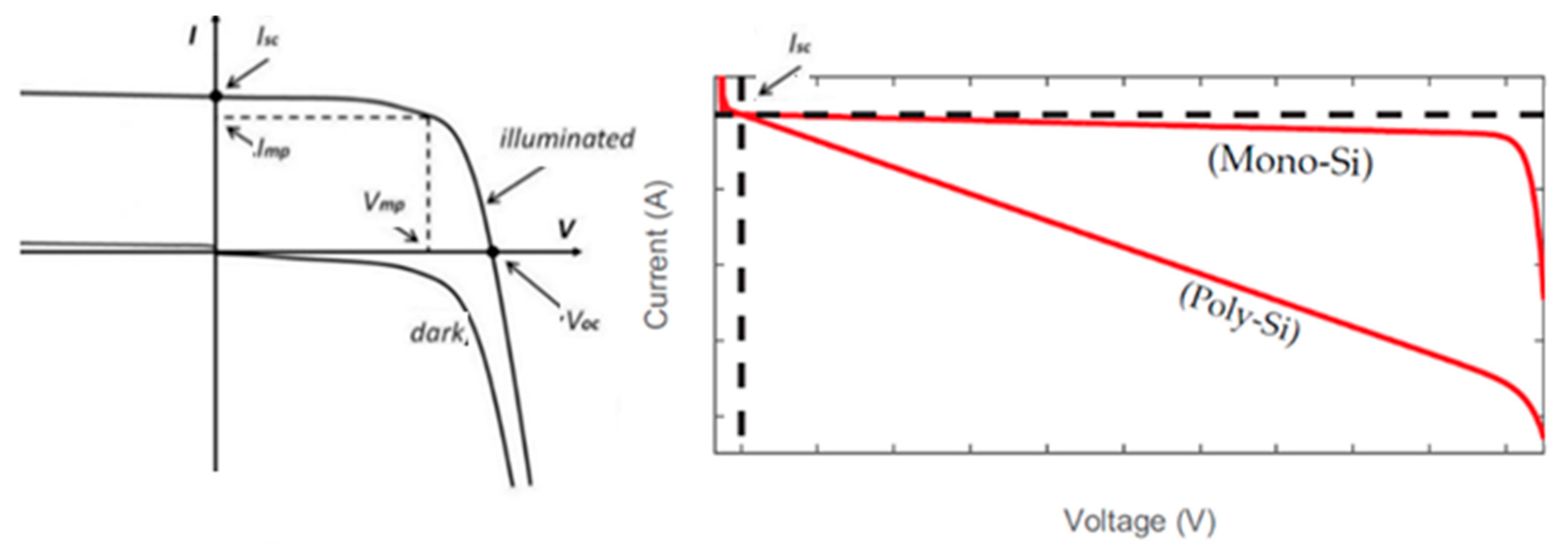
The reverse bias characteristic of a PV cell, presented on
Figure 1, is very important to understand what happens when the cell is not in photovoltaic operation [
1,
2,
3]. The reverse-bias characteristic is heavily influenced by the shunt resistance. This influence has been considered by using standard values for the following two kind of cells: for Mono-Si and for Poly-Si. One main difference is the bigger Rsh of the Mono-Si cells. This makes Poly-Si cells more prone to higher values of current outside of photovoltaic operation, dissipating more power instead of producing it.
The most common used PV panel configuration is a series of cells in a string divided in 2–4 parts, where each one is connected in parallel with a bypass diode (BPD). These panels can then be arranged in different ways, and their energy transformed from DC to AC to be injected in the grids they are connected to. Also, the PV system architecture uses a Maximum Power Point Tracker (MPPT) device, so the system always operates at its maximum power point (MPP).
1.2. Identification and Effects of Partial Shading
Shading is a natural cause of light obstruction, that can lead to some PV systems problems, as power losses [
1,
5]. Partial shading is particularly problematic, since it only reduces the irradiance in certain parts of a PV panel, an example of it, can be seen in
Figure 2. Mitigation techniques have an integral and key role of optimizing peak power production.
There are two possible scenarios, when a PV panel is under partial shading conditions [
1]:
The shaded cells still produce its own reduced power, depending on the shading factor.
The shaded cells may have to carry current of non-shaded cells, causing hot spot effect.
A cell in scenario 1, although not operating near its maximum due to the reduced irradiance received, it “forces” all cells in the series string to operate at the lowest current. They are still operating in the photovoltaic area of the cell characteristic curve. This means, little shading can greatly reduce the power output of an entire panel. However, scenario 2 is the least desirable, considering partial shading on cells. As consequence they stop operating in the photovoltaic region and become forward biased. Depending on the intensity of shade and the number of affected cells, a hot spot may occur [
4]. This situation is easily illustrated on
Figure 1. Basically, a cell can consume and dissipate a lot of power, instead of producing it, when it is outside the photovoltaic mode. This happens since the voltage reverse-bias area the voltage is negative and the current increases greatly.
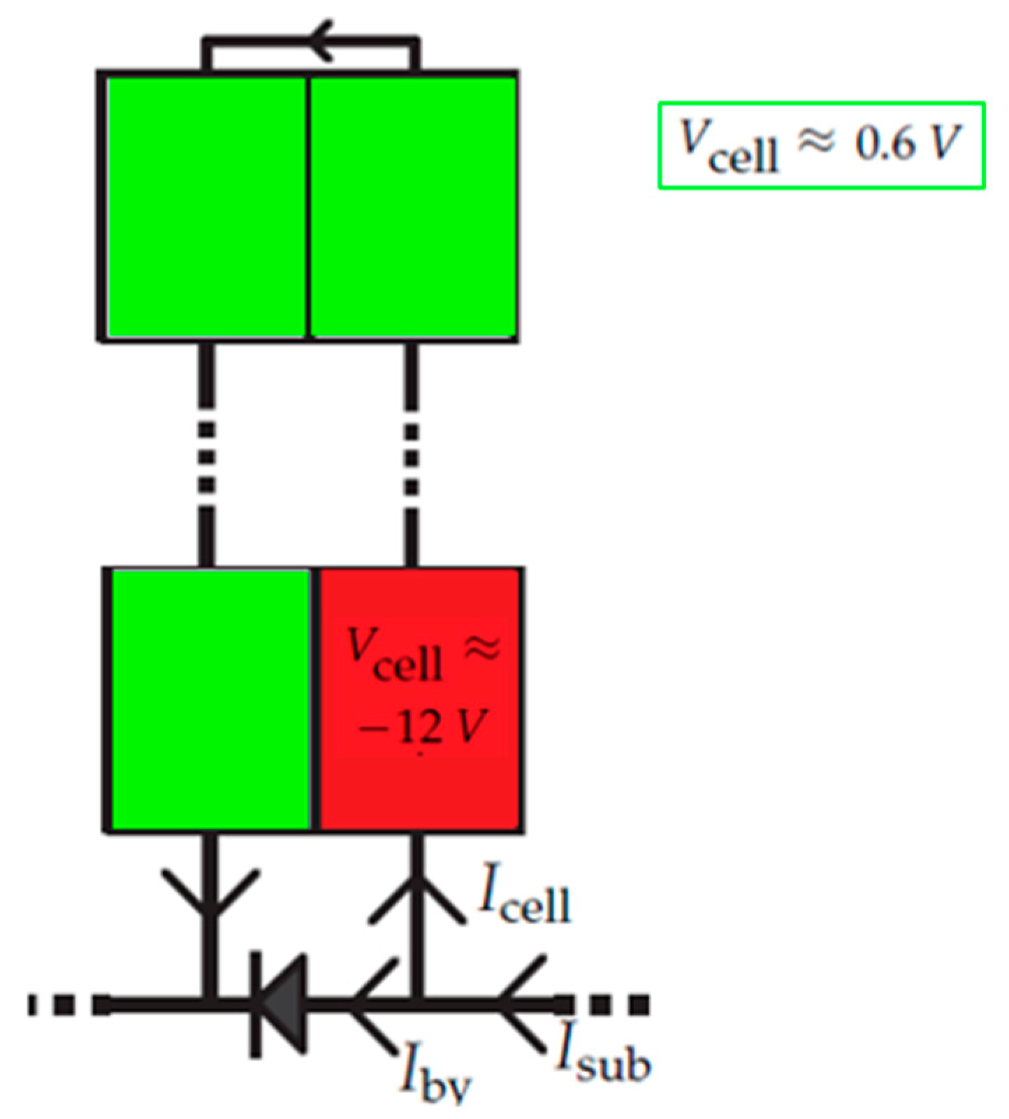
To mitigate it, many manufacturers use BPDs, so the current flow through them instead of the affected substring. Sadly, this does not prevent hot spots. A working BPD imposes a low voltage in its substring and the forward voltages produced by non-shaded PV cells induce a reverse voltage in the shaded parts of the submodule,
Figure 3.
It is possible to observe in
Figure 3 an example of that, with 20 cells in series in a substring, where it is induced a voltage of 19 × (−0.6) + (−0.6) = −12 V across the mismatched cell. If a reverse current of the cell is I > 0, the affected cell could dissipate a large amount of power. In worse cases, this can lead to the destruction of that part of the panel, burning it [
1,
4,
6].
Using BPD in PV panels generates another problem, since the Power-Voltage Curve, as observed on
Figure 4, presents multiple local peaks instead of only showing the global peak, the MPP. A MPPT has the objective to locate the power peak. Undesirably, the output power from partially shaded strings is often reduced, due to the probability of the MPPT algorithms selecting a local peak.
2. Methods to Mitigate Partial Shading in Literature
2.1. Panel Interconnection Topologies
A PV array is usually formed by a series/parallel configuration of modules. As for cells, a shaded panel in a string will lead to similar power losses. So, [
7] proposed to find out which topologies are more advantageous under partial shading conditions. Several other configurations have been discussed, such as series-parallel (SP), total cross-tied (TCT), bridge-linked (BL) or honeycomb (HC), compiled on
Figure 5.
Analyzing the effects of the bypass diodes, tests were made with and without them for a 6 × 4 array. For a broader and better understanding, diverse and detailed tests were conducted for 10 different array sizes and 15 different random shading patterns were assigned for each array. For these cases, it was considered one BPD across a group of 36 cells, one per module. There was a second test using two BPDs per module for 15 random shading patterns of a 6 × 4 array.
The many analyses done for the different array configurations in [
7], indicate that in most cases TCT provided a higher power output compared to the others. Conclusions from this study were that TCT is the best configuration closely followed by HC. Generalizing, TCT is the best configuration for symmetrical arrays and HC for asymmetrical ones. The worst was SP.
2.2. PV System Topologies
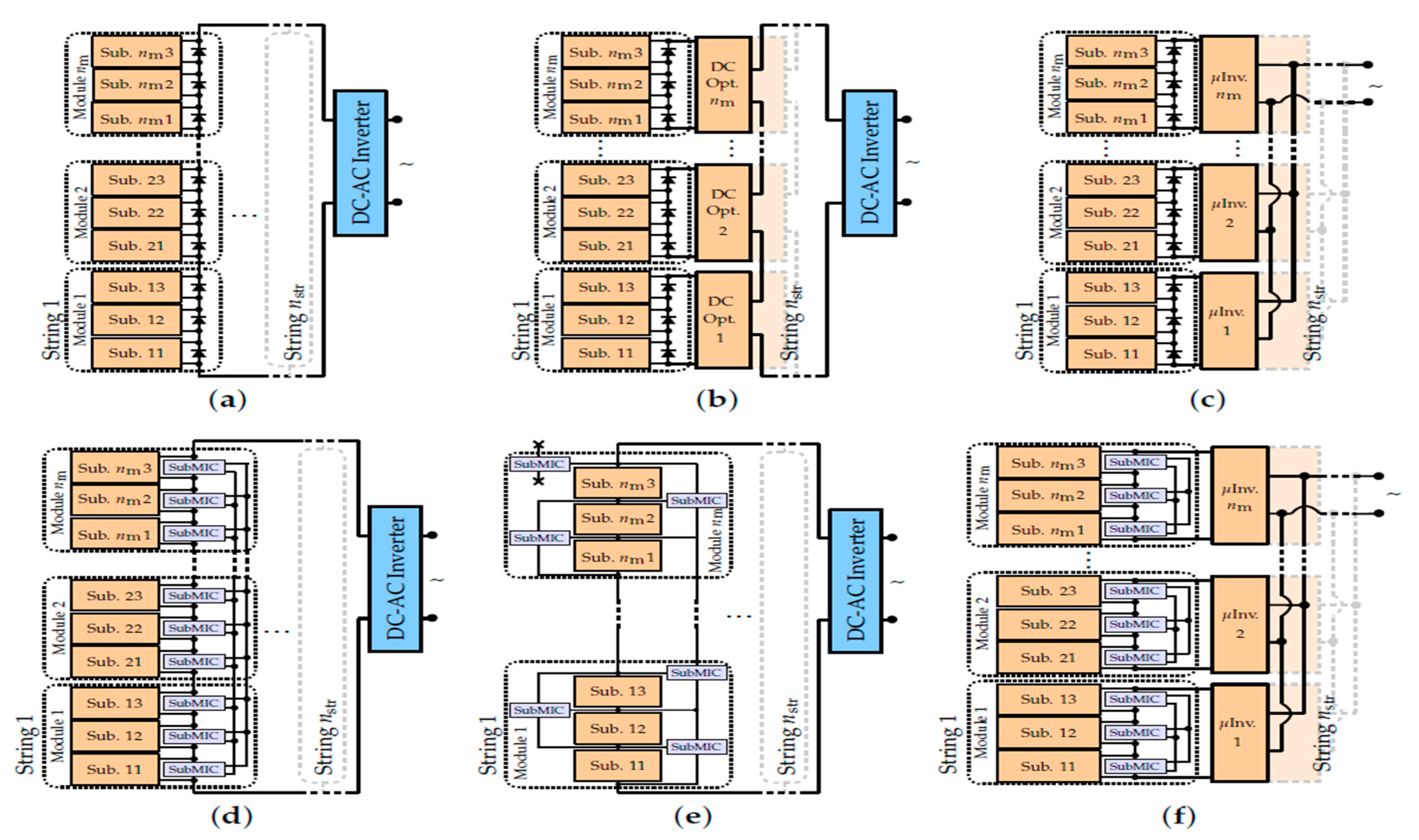
Another way to mitigate partial shading is by using different PV power electronics architectures, as presented on
Figure 6 [
1]. The most conventional method used is the string-level inverter (6a), plus BPDs. Other solutions can be using full power processing (FPP) DC optimizers (6b) or microinverters (6c). These solutions work at the module level (FPP MICs), which limit the effects of mismatching, but may not always prevent bypass diodes from activating, and consequently creating hot spots.
Although, at submodule level, these converters (FPP subMICs) replace the BPDs, maintaining the submodules’ operation at their MPP. Despite reducing the probability of hot-spot occurrence, these converters must process the total power of the PV system. To overcome this limitation, there is differential power processing (DPP). The mismatched power is passed from one submodule to another, mitigating it and using low rated converters, reducing system’s costs and size. Several methods can be used: PV-to-bus subMICs (6d–isolated-port version) and the PV-to-PV subMICs (6e). The latter was not considered in [
1] due to limited power ratings. Finally, there are the subMIC-enhanced microinverters (6f), where BPD are replaced by DPP converters, and each module has a microinverter.
In [
1], the objectives were quantifying the probability of hot-spot frequency under partial shading; quantifying how well hot spots were mitigated; and how hot spots affect the system’s lifetime and its reliability. From the results attained all distributed architectures decrease the occurrence of hot spotting. The best results were from submodule power converters. In conclusion, distributed power electronics provide many benefits, from increasing the energy yield to preventing hot spotting, improvingt the system’s lifetime and reliability.
2.3. Other Techniques
There are other PV system topologies, like the state-of-the-art review presented in [
8] indicates. These offer new different advantages, although, some have more complex and costly electronics architecture or they imply bigger levels of control and software associated.
Several techniques are related to how the Maximum Power Point Tracking (MPPT) is done. It is tough to select a specific MPPT technique as the best, since all methods, as reported in [
8], all have their own advantages and drawbacks. So, the best option is always deciding according to the project scenario.
Some other separate techniques are also present in the literature, as complex electronic circuits that optimize the power output of a PV panel [
9,
10] or testing different BPDs configurations [
11]. These circuits replace the BPD, working as an intelligent switch. There are still efforts in the development of BPD in modules, testing new kinds of materials and testing different interconnection configurations for different shading situations.
2.4. Economic Overview and Overall State-of-the-Art Discussion
Comparing the solutions, economically, can provide insights in terms of costs-benefits, that are as important on par to the technical advantages, since the objective of energy production systems is to produce energy cost-efficiently. For example, the extra cost of cabling to interconnect the panels is not significative since the cost of DC cabling is around 2€/m and the increase of energy produced justifies such investment.
In 2018, the most common situations were central/string inverter for commercial/utility solutions, although some commercial already are already investing in DC optimizers [
12]. Although microinverters are more expensive, they get better results than DC optimizers and the latter gets better results than conventional systems. The higher production of a microinverter system is converted in an economic advantage over the expected lifetime of the PV system. The LCOE example in [
13] shows that the benefits of higher production of energy outweigh the higher costs. When the cost of replacing the central inverter is considered, this difference is even greater. The microinverter also offers safety advantages, which were not monetized in the calculation. Another example [
14], the LCOE and NPV values of the project were calculated. The microinverter option is always best and in the case of partial shading the gap becomes better. As prices decrease, these solutions become more viable for bigger installed capacities, such as commercial systems.
As for the newer power electronic systems, such as DPP and FPP subMICs, no economic case studies were found. Although, [
15] studied the advantages in order to decrease the LCOE, improve the systems’ reliability, and increase their lifetime.
3. Models Used Continuously in the Simulation Work
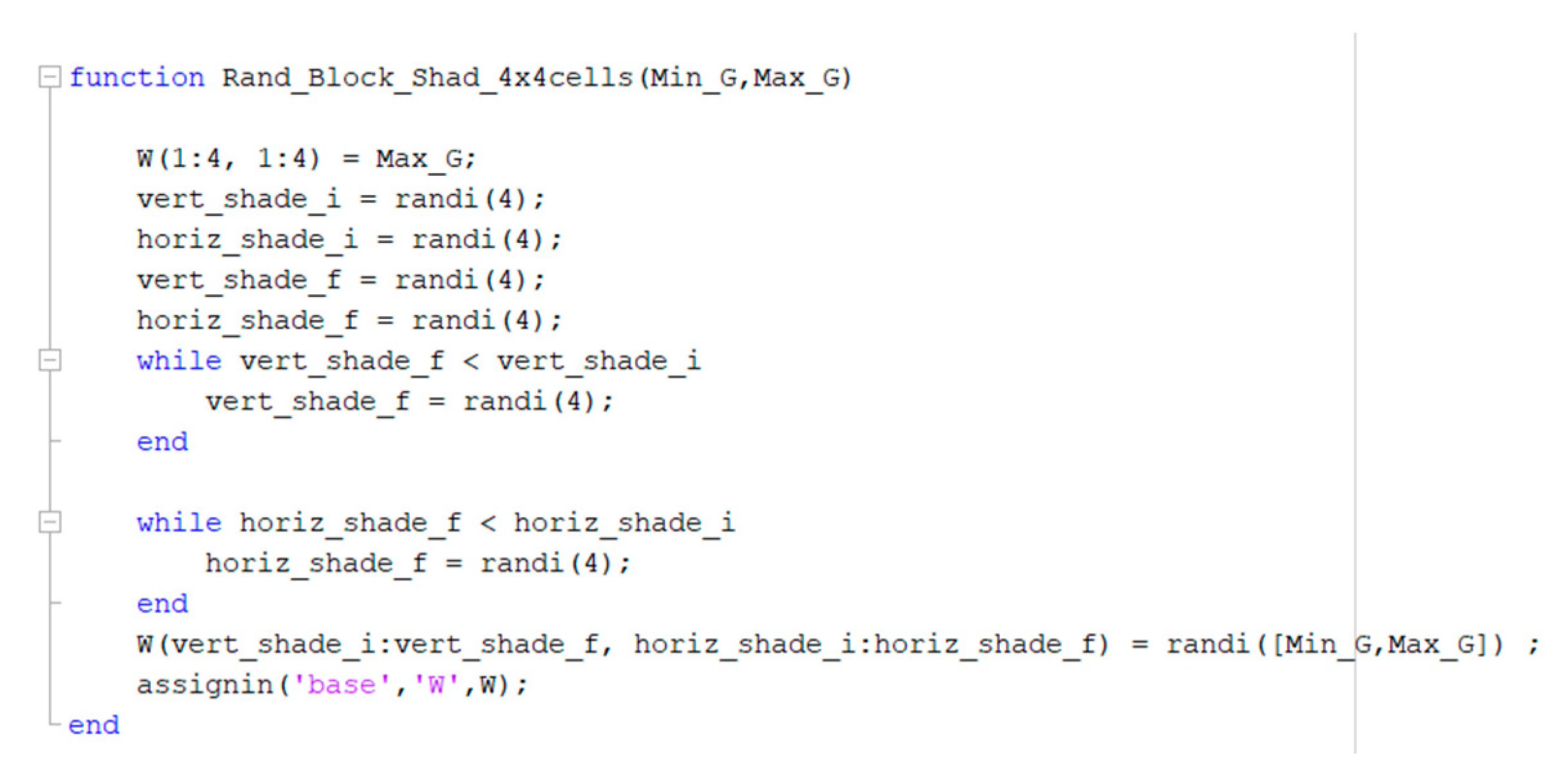
The simulation work was conducted using MATLAB and Simulink. The first step was to create an algorithm model that could randomize the partial shading size, percentage of shade, and the position where it would occur in the panel, observed on
Figure 7. Then, it had to run the model several times for each situation and under similar conditions.
This algorithm receives as input the minimum and maximum irradiance and releases as output a matrix, W, with the cell’s irradiance in each position with a random partial shading. Firstly, it creates the matrix, W, with the wanted panel size, and all positions with the maximum irradiance value. In this case, it has a total of 16 cells arranged 4 by 4. After, using the randi function from MATLAB, it is possible to randomize the size and location of the partial shading by randomizing a number for the initial and final position on the vertical and horizontal axis of the shading matrix. This process is executed in a WHILE loop, preventing that the randi chooses a final position value smaller than the initial. Finally, within the first matrix created, W, the values in the positions obtained by the previous process are changed to a randomized value between the minimum and maximum value of irradiance from the input. Then, the output matrix W goes to the MATLAB workspace.
Some simulations were intended to have a constant percentage of partial shading (20%, 25% or 50%). So, it was necessary to create an algorithm capable of such, which is presented on
Figure 8. This decision was made to compare the different models tested in conditions where the partial shading was more likely to happen;for example, to observe if the size of the partial shading could make a specific topology more interesting in reducing power losses.
This algorithm is built upon the first, so it receives the previous input of irradiance plus the partial shading percentage. The output is the same matrix W, with the cell’s irradiance with a random partial shading. The algorithm creates the same initial matrix but then there are IF conditions to select which of the partial shading percentage was introduced as input. After, the algorithm selects the shade size by searching within a loaded mat file that has specific values for initial and final values that correspond to the possible ways of creating a grouped partial shading of the percentage given. Then the process is similar again, the location of the partial shading and its value are chosen randomly, sending a new W to the MATLAB workplace.
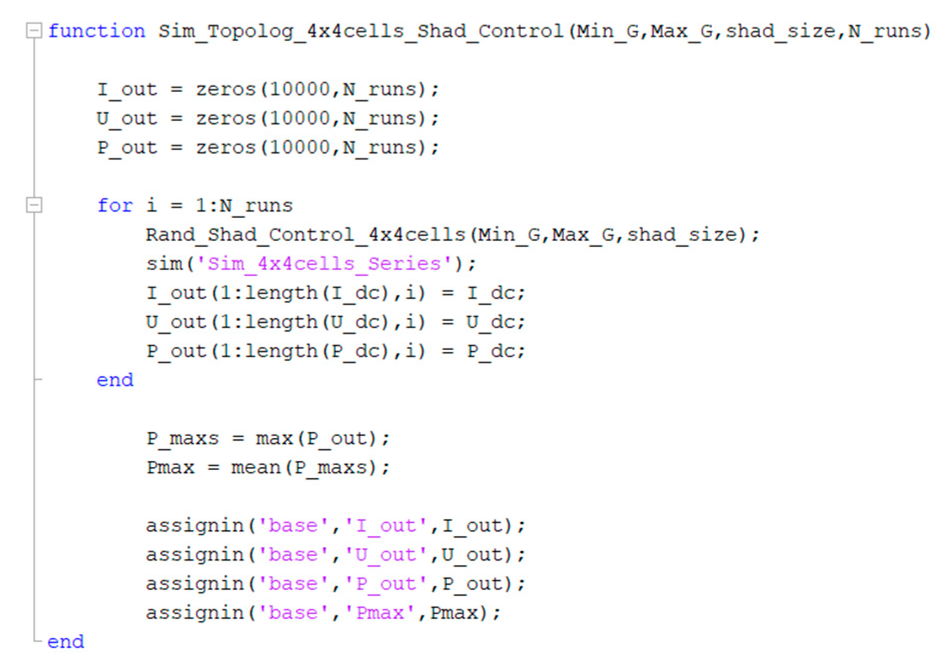
The rest of the model is comprised by a Simulink model of the case being tested and an overall function created to run both the function responsible for the random partial shading creation and the PV cells/panels model being tested, which is presented on
Figure 9. The inputs needed are the ones the partial shading randomizer needs plus the number of runs. Basically, inside a FOR loop the function runs the partial shading randomizer for the number of runs given, followed by the Simulink model, and each time saves the results inside a matrix, previously created, with the size of runs given. Its output is the compiled matrices of current, voltage and power, as well as the computed average of the MPP. The latter will be used to compare the different topologies.
4. Alternative Cell Interconnections in PV Cells
Although it was not discussed in the literature found, the following idea was envisioned: What if the cells within a PV panel were arranged in different topologies as for panel interconnection? The simulation work will focus on comparing different, array sizes, partial shading percentage, and PV cell technologies. After, some experimental work was conducted to verify some results. It was decided to simulate some scenarios similar to the experimental work, to attain some comparations. So, a “custom PV panel” of 16 cells was created.
4.1. Simulation Work
The cell model used for the simulations of this section was the solar cell model of the Simulink library, which has built-in the 1M5P PV cell model, the parameters needed for input in this model and that were considered were the irradiance-W, the short circuit current, ISC, the open circuit voltage, VOC, the ideality factor, N, and the series resistance, RS. The shunt resistance, RSH, is already considered by the model.
The first set of simulations are associated with the small Mono-Si cells present in the laboratory which will be used also in further experimental work. These cells, under the conditions of irradiance 1000 W/m2 and cell temperature of 40 °C, have the following estimated parameters: ISC = 123 mA, VOC = 2.12 V, N = 1.95, and RS = 5.5 Ω. This set of simulations was done to 4 × 4, 4 × 5 and 5 × 4 array sizes and it is separated in the following categories of Partial Shading Size:
Random Size Partial Shading
Constant 20–25% Partial Shading
Constant 50% Partial Shading
In each of the categories the following topologies will be tested:
The results will present the average maximum power for two simulations of 250 runs each. This is to assure the average quality of the partial shading randomizer, by applying an extensive set of partial shadings and by double checking the results. The number of runs is justified by the maximum difference of 0–2% between the same topology simulation and due to the large amount of time necessary to run the models. An example of a Simulink model can be observed on the
Figure 10.
Each result is already the result of 250 examples of partial shading cases, and consequently each maximum power output is compiled by the FOR iteration, and the final result is the mean of such matrix. The results are two simulations to recheck and assure the average quality of the partial shading randomizer, by applying an extensive set of partial shadings and by double checking the results. The maximum difference of 0–2% between the same topology simulation guarantees it. To reduce this difference and achieve near 0% differences would take a lot more runs and this method was preferred due to the large amount of time necessary to run the models.
The results on
Table 1 will also present the losses, in percentage, compared to the no-shading case, and the advantage, in percentage, over the standard Series + BPD topology.
From the results obtained is possible to verify that, as expected, the topology best fit to help mitigate the effect of partial shading in most categories was TCT, closely followed by BL. TCT also presented the best results for the Random Size Partial Shading category across any array size, while BL was consistently best during heavier partial shading, even surpassing TCT in 2 cases.
The new topologies offered less advantage, as expected, when the number of BPDs increased and when the percentage of shading was higher (50%). Also, in practically every category, any topology had less power losses than the standard topology, even in this set of simulations where it was used 4 BPD for 20 cells, which is not common in commercial PV panels.
The other set of simulations was done for three current main different commercial PV technologies present in the market. Industry standard modules are composed by 60 cells + 3 BPD.
This set of simulations is separated in the following categories:
In each of the previous indicated categories the same topologies will be tested. The standard Series topology will only have 3 BPD as commercial PV panels. All simulations were in the conditions of irradiance 1000 W/m
2 and cell temperature of 45 °C. The parameters from each technology on
Table 2 were obtained from the PVsyst database, from the following panels:
Mono-Si (2020)-Trina Solar TSM-DEG5-(II)-280 W
Poly-Si (2017)–Trina Solar TSM-330PE14A-330 W
HIT (2019)–REC Solar REC350AA-350 W
Regarding the technologies, it is important to point out that the HIT technology is comprised of 60 half-cut cells, meaning the panel has 120 cells, each one with half the size of “standard cells”. Then the panel is divided in two groups of 60 cells in series that are connected in parallel. This allows to distribute the stress under partial shading while using only the standard three BPDs, decreasing the power losses. One example of a Simulink model can be observed on
Figure 11.
The results on
Table 3 will present the average maximum power for two simulations of 250 runs each. That number was decided by the same reasons as previously and also because these models’ run is even more time consuming, particularly the HIT technology, since its Simulink model is more complex.
Yet again, as expected, the topology best fit to help mitigate the effect of partial shading was TCT, in five out of nine categories. Once more, closely followed by BL, with two out of nine. TCT presented the best results for the Random Size Partial Shading category across any technology type, while BL was best in cases of a constant higher percentage of partial shading (50%). Moreover, in the category Constant 25% Partial Shading for the HIT technology, the HC topology was the best. In this overall category, the HC topology was usually close to TCT and BL.
Once again, in practically every case, any topology had less power losses than the standard Series + 3 BPD. Important to note, that the advantages are lower for the HIT technology. Nonetheless, this is true even for the complex twin panel design.
4.2. Experimental Work
4.2.1. Small Mono-Si Cells
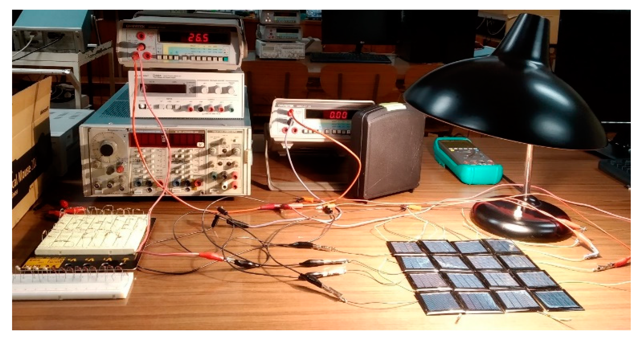
As mentioned before some experimental work was conducted to verify the MATLAB results. For that, 16 small mono-Si cells were used to create a “custom PV panel” to test and verify the simulations results. Additionally, to the 16 cells, the following material was used: two multimeters, one in series to measure the current and the other in parallel to measure the voltage; several wide-ranging resistances in order to create different loads; a lamp to create irradiance; an irradiance meter; and connector cables. The workstation can be seen on
Figure 12.
The resistances are important to the method used to obtain the I-U and P-U curves of the panel, since each load corresponds to a specific point of current and voltage of the curve. Enough points acquired create a significant plot for each configuration.
Since it would be very time consuming to test several array configurations, one of 16 cells in an 4 × 4 array was chosen. The same applies to the shading patterns, choosing five to compare. A base No Shading test at 350–400 W/m
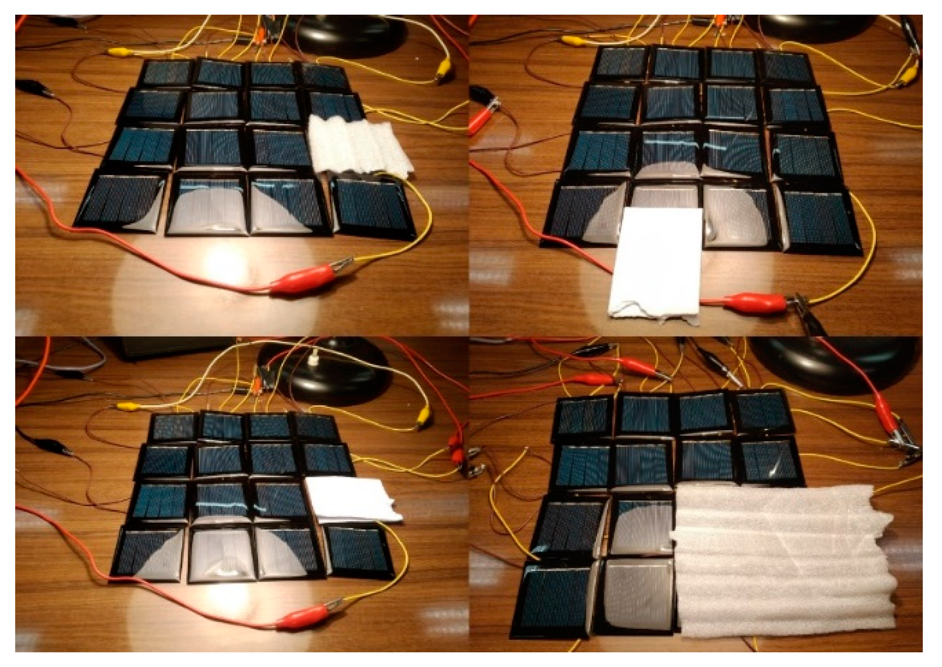
2 was best achieved in the laboratory for these small cells, without compromising them with the heat caused by the lamp and the cells’ operation. Plus four partial shaded tests, as verified on
Figure 13:
Soft Shading in one cell (created with a foam sheet, that reduced the irradiance to half–180–200 W/m2)
Hard Shading in half a cell (created using a folded paper, that reduces the irradiance to nearly zero)
Hard Shading in one cell (created using a folded paper, that reduces the irradiance to nearly zero)
Soft Shading in four cells (created with a foam sheet, that reduced the irradiance to half–180–200 W/m2)
Naturally, for each test, all the topologies were tested. Including the series topology with 2 BPD and without. The cells were welded in strings of four to prevent the connections to detach. The other topologies were made using connector cables. For the BPD case, each one was connected to a group of 8 cells.
Starting the experiment, the I-U curve differences between the standard series topology and the others was observed. As expected, the new presented topologies have a four times higher total current and four times lower total voltage. The results on
Table 4, have the MPP’s for each topology, as well as the advantage comparisons to the standard topology.
In all experimental tests the best topology to mitigate partial shading power losses, as expected, was TCT, closely followed by BL, and then HC followed by SP. Consistently showing up as the worse is the Series + BPD, despite offering better results than the standard Series topology, especially hard shading cases.
These results validate the MATLAB model used and also verify the results obtained from analogous simulations, since all non-standard topologies are better at mitigating partial shading. And because the two best topologies continue to be TCT and BL.
These tests advantages appear greater than in the simulations. This is because for the Series + BPD topology only two BPD were used versus the four in the Simulink model. Secondly, the test cases chosen are largely more advantageous for the non-standard topologies since the partial shading is low and small unlike in the MATLAB simulations where the results were an average of hundreds of random partial shading patterns.
4.2.2. Perovkite Cells
To test other types of PV technologies, another set of cells were experimented on, perovskite cells. These are a type of solar cells comprised of a perovskite-structured compound. Furthermore, these cells have a different characteristic curve illustrated on
Figure 14.
An equal “custom panel” of 16 cells, from infinityPV, was created and the same equipment and methodology to conduct the experiment as before was utilized, except for an additional second lamp, as seen on
Figure 15. However, this set of cells were not welded together, the terminal connections are very thin slates of silver that made impossible such task. The solution used was small copper cables set in place by small stickers. Unfortunately, due to the heat produced by the lamps, the stickers lead to contact issues. This led to longer duration tests since it was necessary to find and re-establish such contacts each time. Additionally, since the cells are bigger in area there was the need for a second lamp, so, the variations of irradiation among cells were higher. This meant it was difficult to maintain exactly the same conditions throughout the tests. To get better and more coherent results the comparisons for cases of partial shading were done to the No Shading test case of each topology, instead of an average of all topologies, as previously done.
The set of tests included a comparation base test without shading, with irradiance around 350–500 W/m2. Additionally, three partial shaded tests were chosen:
Soft Shading in one cell (using a foam sheet, reduced the irradiance to half the no-shading–200–300 W/m2)
Hard Shading in one cell (using a carboard, reduced the irradiance to practically zero)
Soft Shading in four cells (using a foam sheet, reduced the irradiance to half the no-shading–200–300 W/m2)
Once again, it was deemed interesting to observe the I-U curve differences. However, the new presented topologies (10–11 mA) do not have exactly four times the total current of the series topology (3 mA). The difference is even greater in the total voltage, the new topologies with 2.5–3 V and the standard series topology with 21 V. Furthermore, opposite to the mono-Si cells, the MPP’s for the case without shading are not similar and oscillate among topologies. This reenforces the idea to compare the results using the no shading case for each topology. For each shading category, all the previous topologies were tested.
The collected results from the tests conducted, are on
Table 5. Although, this time only the Series topology was considered for comparison since the BPD are not as important for this technology. The cells even if at 0 W/m
2 still carry the other’s current, making their use for this pointless.
Observing the results from the perovskite cells tests set, we can conclude that yet again all non-standard topologies achieve higher MPP. However, for all tests ran, the best topology to mitigate partial shading effects is the HC topology.
Despite not having done simulations, it was relevant to verify that this technique helps mitigate partial shading for other technologies, such as perovskite solar cells. It is possible to conclude that even across other technologies nonstandard topologies offer better results than the current market solution.
5. PV Panels Interconnection Topologies
In VI the objective was to test and compare different PV panels interconnection topologies under partial shading, as depicted in the literature previously presented. So, the simulation work focused on comparing different, array sizes, percentage of partial shading, levels of irradiation, and PV technologies.
Then, some experimental work was conducted to verify the first results. To simulate some scenarios similar to the experimental work, 6 CdTe panels were used. The panel’s parameters were from one similar to the one tested in laboratory.
5.1. Simulation Work
The simulation model used for the simulations of this section was different from the previous. A PV panel model was created from scratch applying the 1M5P model, using a current source, a diode and two resistances. For this model, the necessary parameters are the short circuit current, ISC, the inverse saturation current, IS, the diode ideality factor, N, and the series and shunt resistances, RS, and RSH, respectively. This first set of simulations done for 3 × 2 and 2 × 3 array sizes were separated in the following categories:
In each of the previous indicated categories only the topologies Series, SP and TCT were tested. Only these because for an array size smaller than 4 × 3, the BL and HC topologies cannot really express their configuration. These array configurations were chosen since the maximum number of panels in the laboratory for experimental tests were only seven, so, the biggest arrays possible were 2 × 3 and 3 × 2. Although, simulations with a third array size (4 × 4) were also done, to simulate all topologies.
Two levels of irradiation were chosen to depict a realistic PV system scenario: High Level of Irradiation (800 W/m2) for average summer months and Low Level of Irradiation (400 W/m2) for average winter months or low-light countries.
All simulations were conducted with a panel temperature of 45 °C. The parameters from each technology were obtained from the PVsyst database on
Table 6, from the following panels:
Regarding the technologies, it is important to point out that the CdTe technology used in the simulation is comprised of 116 Cadmium-Tellurium cells in series. The results on
Table 7 present the average max power for two simulations of 500 runs each. They have the losses, in percentage, compared to the no-shading case, and the advantage, in percentage, over the “standard topology”. One Simulink model is on the
Figure 16.
It is possible to verify that, as expected, the topology best fit to help mitigate the effect of partial shading, in all categories, was TCT. It is also possible to point out that all panel configurations presented less power losses in the 2 × 3 array size, this is particularly obvious in the SP and TCT topologies.
The other simulations set (4 × 4 array) were only for the Mono-Si technology, in order to test all topologies. Alongside High and Low Irradiation, it is also separated in partial shading sizes:
Random Size Partial Shading (random number of panels shaded)
Constant 25% Partial Shading (four panels)
Constant 50% Partial Shading (eight panels)
As previously, the results on
Table 8 will present the average max power for two simulations of 500 runs each. From the results of this set of simulations the best topologies to help mitigate the effect of partial shading were TCT and HC. However, the differences among the non-standard topologies were usually small. HC presented stronger results in heavier partial shading patterns (50%). As before, all topologies achieved better results than the standard topology.
5.2. Experimental Work
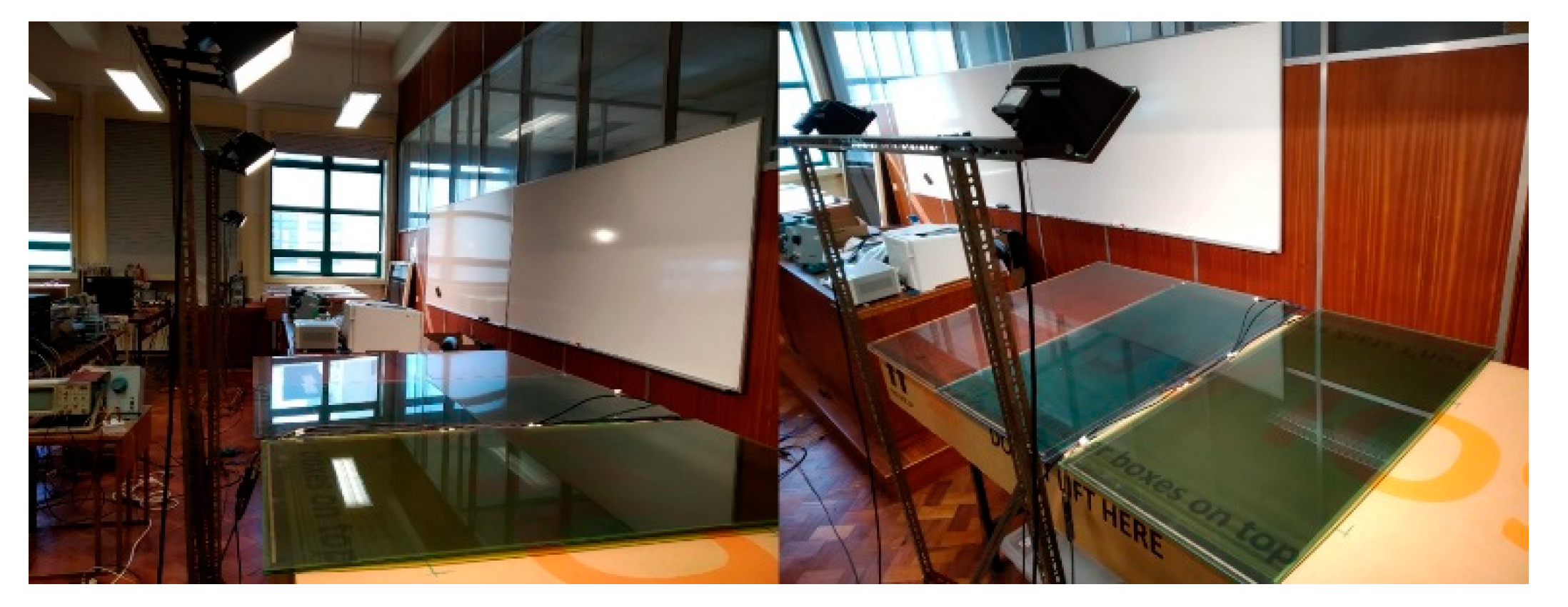
In order to experiment and verify the MATLAB results, the idea was to use 6 CdTe panels of 40–48 W panels to test the Series, SP and TCT topologies. The HC and BL topologies were not considered because there were not sufficient panels to properly create them.
Other equipments used were the searchlights for irradiance, cables and multimeters on
Figure 17.
There were not high enough rated resistances, in the laboratory, to use as load to create the I-U Curves as in the section before. Although, there was an attempt to connect the PV array to the grid, nfortunately, the inverter in the laboratory had not high enough voltage to connect the array and use the grid as the load. So, the maximum power was also not possible to obtain.
Leaving the only option to be measuring the VOC of each case and comparing it with simulation data. The tests conducted were:
No Shading (irradiance at 180–200 W/m2)
Hard Shading in half a cell (created using a black cloth, that reduces the irradiance to practically zero)
Hard Shading in one cell (created using a black cloth, that reduces the irradiance to practically zero)
The results on
Table 9 obtained from these panels cannot be compared directly with the MATLAB simulations because the panel parameters are not equal. It is the best scenario possible.
Examining the results, as expected, the VOC from the Series topology is always higher, around double the size of the other two topologies. Also, it can be observed that the TCT topology has a slightly higher VOC’s than the SP counterpart. It is also possible to notice that, similar to the simulations, the VOC variation to the Series topology in the Hard Shading-One Cell set is slightly below 50%. Despite this not being an exact comparation of maximum power and the differences in resilience of each topology in the face of partial shading, it is a good validation on the MATLAB simulation models. So, the results obtained there are reliable as proven by the similarities in the VOC’s experimental behaviour.
6. PV System Topologies
In this section the objective was to test and compare, under partial shading, different PV system topologies, associated to different power electronics, as depicted in the literature previously presented. Although, contrary to VI, this work focused only on MATLAB simulation. The simulation model used for the simulations of this section is the same as the one from VI. The panels’ input data used in the simulations was also the same as the overall cross-categories, in order to better compare the results of this section with the previous one. The following topologies were tested:
The results present the average MPP for two simulations of 500 runs each. For the PV system topology Series + DC-DC converter, a Boost converter from the Simulink Simscape library was placed in the Simulink model (
Figure 18), so to simulate panel’s power optimizers currently in the market.
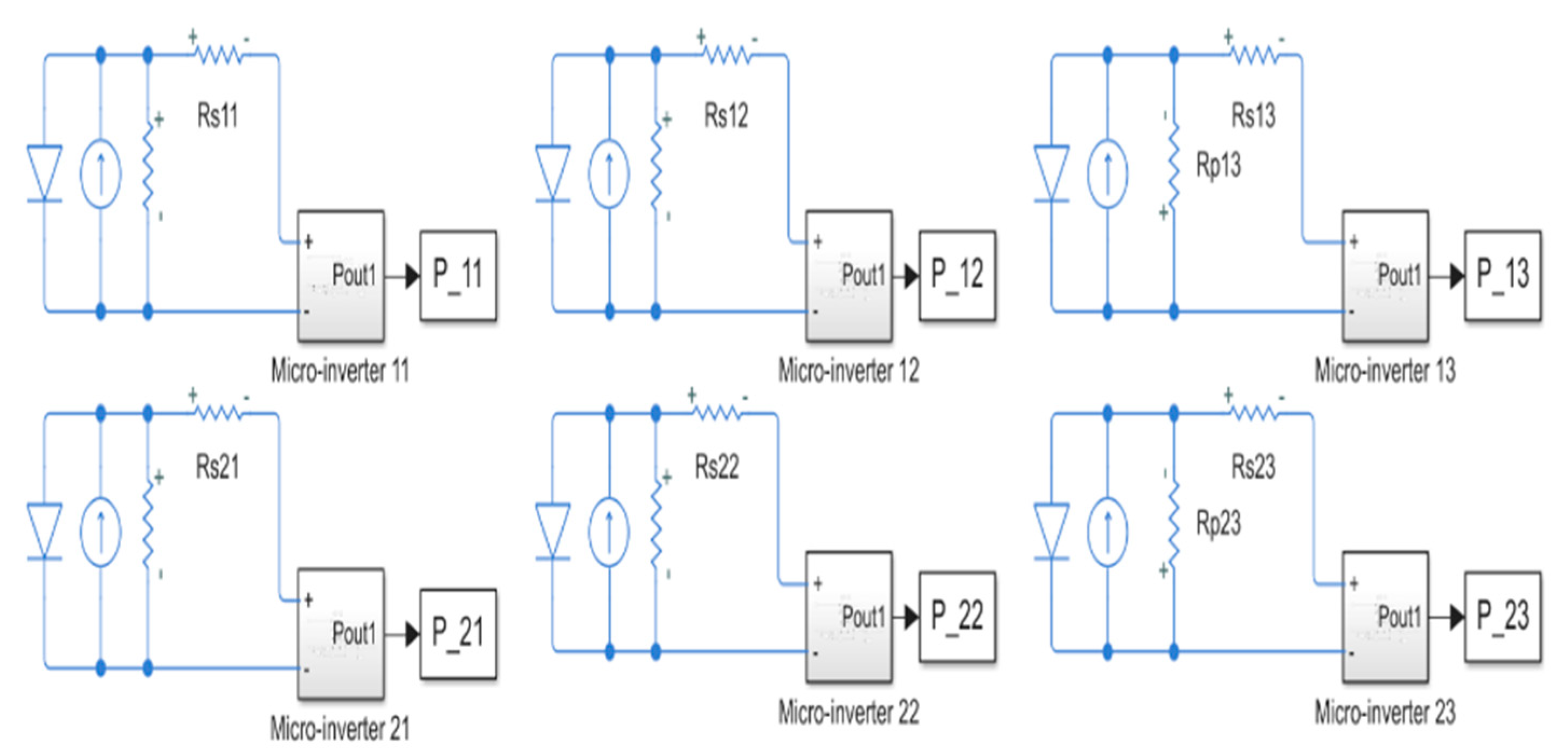
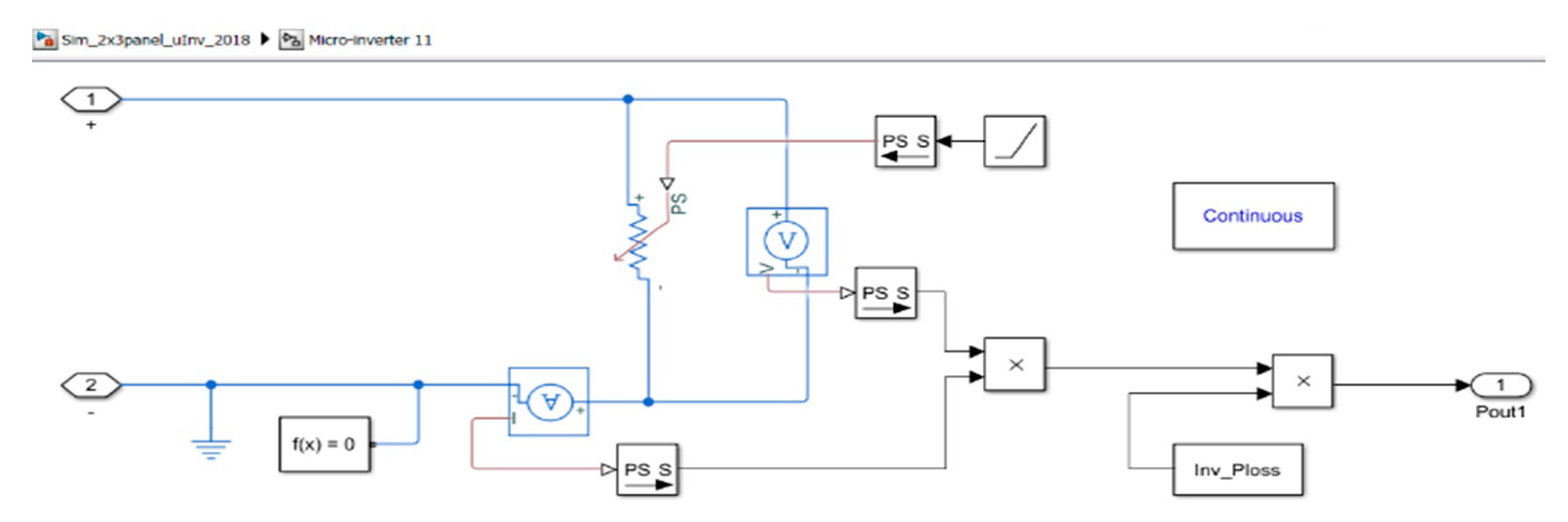
For the µ-Inverter, due to the inexistence of a single-phase inverter in the Simscape library, a simple block was created, as verified on
Figure 19 and
Figure 20, meant not to emulate an inverter operation, but to single panel independency. This means each “µ-Inverter” block gave the total power from each isolated panel, multiplied by a factor of 0.95, representing inverter power losses. The results regarding PV technology comparation, are in
Table 10.
From the results obtained in this set of simulations, the best PV system topology to mitigate the effects of partial shading is the µ-Inverter topology. As expected, µ-Inverter topology is the best of all, even comparing with topologies like TCT or BL. It is even better since only here were considered inverter power losses. As for all others, the results are for DC power, to connect to the AC grid, they too would have to account inverter power losses. The DC-DC topology fell short from expectations, as even some interconnection’s topologies had better results.
Contrary to the interconnection topologies, there were constantly better results in the 3 × 2 array rather than in the 2 × 3 array. This may indicate that power electronics topologies are best suited under partial shading of small arrays having more lines than columns. For interconnection topologies it is the opposite.
The results of the set of simulations on
Table 11 are regarding different percentages of constant partial shading, only for the Mono-Si panels.
Once again, the best results came from µ-Inverter topology, reaching even higher average power values than previously. Since this was also observed in VI, it is now possible to argue that the bigger the array, the bigger the advantages of mitigating partial shading via non-standard topologies. Once more, the percentage of advantage over the standard topology decreases when the constant partial shading increases.
There was an advantage of the DC-DC topology over the panel interconnection topologies in the 25% of partial shading case. However, under heavy constant partial shading, it is the second worst, which makes sense since it is still a Series topology.
7. Critics to the Presented Techniques
The previous presented techniques to mitigate partial shading in PV panels have without doubt several advantages over the current market standard techniques. Although, it is also relevant and truthful to discuss the downsides of such techniques.
Regarding the cell interconnection topology techniques, despite the lack of need for BPDs, there is the need of more research for the long-term results in PV panels, due to the higher currents flowing in the cell’s connections (6x times higher). Additionally, there are higher costs associated with changing the standard operation of the industry. From the projectionist and installer side, there are also different requirements, either for cables or inverters, which could require, higher costs.
Concerning the different panel interconnection topologies technique, it does not offer any specific barriers and has many upsides as seen in VII. However, there is the need to be attentive from the installer/projectionist side, in choosing an appropriate inverter capable of withstanding higher currents, although the SP topology is already being used in PV projects nowadays.
From the techniques involving power electronics, the biggest barrier is still the higher costs. Although the DC-DC topology offers a good panel’s operation isolation, it is not the same as the provided by the µ-Inverter topology. Unfortunately, this is equally true to their higher costs. Nevertheless, as the research in III indicated, in the long term, µ-Inverters still have an advantage in higher yields and returns on investment.
Other options were also contemplated, although after some experiments there was not enough processing power to conduct these simulations on MATLAB/Simulink. These included:
Integrating the DC-DC topology with different interconnection topologies
Integrating cell and panel different interconnection topologies simultaneously
Integrating the DC-DC topology with cell and panel different interconnection topologies simultaneously
Sub-mic topologies (DC-DC and µ-Inverter’s topologies applied to sub-module level, as in III)
Apart from these discussions, the most important take from these is the need of further studies in this field, either from simulation work or real-life testing. They are needed to better understand what the new and improved ways to overcome the effects of partial shading could be, and to take a bigger advantage of PV technologies in this energy switching world.
8. Conclusions
The simulation work conducted allowed to corroborate the findings in the literature, of some techniques, such as different panel interconnection topologies or the use of distributed power electronics. This was done, analyzing the advantages and disadvantages for different technologies of PV panels under different operating conditions (Mono-Si, Poly-Si, Cd-Te and Perovskite). From the work realized, the TCT topology for panel interconnection is the overall best bet to mitigate partial shading, considering the performance/cost ratio.
The more relevant conclusion was certainly the technique involving different cell interconnection topologies, that could offer higher power outputs under partial shading, having the best scenario in the TCT topology. However, there is the need of further studies on this technique. It should consider the probability of partial shading occurrence and the longevity of these envisioned panels, due to higher output currents. Although, in this category, TCT may even be interesting for no shading cases, since, as already shown, for low irradiance situations it may provide a higher panel power output.
Concluding, when choosing the best technique to mitigate partial shading it is important to always consider the performance/cost of each for the specific project. That is since, a private home with trees shading is not the same as a large-scale power production in a deserted area, in terms of shading or even investment. Perhaps the biggest conclusion is that the PV system client/designer needs to analyze its own requirements and constrictions in order to decide which of the many available techniques suit its case better.


 ,
, 


