1. Introduction. Traffic Calming
Road planning, together with intelligent transport systems, helps to minimise the negative impact of motorised traffic. Moreover, data acquired from traffic control, such as traffic flow information or video footage of the road network, give a background for traffic modelling. In this paper, we used the video detection of traffic-calmed roads to produce the trajectories needed to build a microsimulation model. Later, we investigated the influence of the traffic-calming measures on traffic assignment.
According to the definition by the Institute of Transportation Engineers [
1], traffic calming is the combination of mainly physical measures that reduce the negative effects of motor vehicle use, alter driver behavior and improve conditions for nonmotorized street users. The reduction in the negative effects comes with the reduction in the main factor causing it—high traffic volume. This allows the reduction in the noise or air pollution and improves the road safety and quality of life. The introduction of traffic calming historically started in the 1960s and 1970s in the Netherlands, Great Britain, Germany and Denmark, and it is connected with the idea to prioritise walking by closing the streets for motorised traffic or to slow car speeds down to walking pace—pedestrianisation [
2].
Traffic calming can be categorised by the scales of influences into three levels [
3]:
Level I—actions restricted to local, residential areas with low traffic volumes and capacities to restrain traffic velocities and to reduce negative traffic impacts;
Level II—actions dedicated to a corridor, which reduces traffic on that corridor, but not on the network;
Level III—actions introduced in a greater area and having an influence at a macro-level.
Recent progress in extracting the trajectories from video footage and the low cost of aerial videography thanks to the growing availability of unmanned aircraft has enabled easy trajectory recording for a relatively large area. This has made it possible to undertake the following research of the influence of the volume–delay function of a traffic-calmed street in order to create a modelling background to answer the question: Is it possible to model a situation where a traffic-calmed street attracts less traffic?
In this paper, the level III influence was discussed. Research on how traffic calming influences the traffic assignment was undertaken. For a given example, through driving characteristics research and microscopic modelling, BPR functions (volume–delay functions in the shape researched by the Bureau of Public Roads [
4]) were estimated—for a street with and without traffic calming. Later, a toy network of two roads of the same length, connecting the same origin and destination, was simulated using an equilibrium traffic assignment method. Simulations were conducted both with the use of PTV Visum software and through individual calculations. The result of this paper was the difference in traffic volume according to the equilibrium traffic assignment in the aforementioned “toy network” as a function of total network traffic volume.
2. Literature Review
2.1. Measurement Methods
The following research requires the fulfilment of two challenges to properly reproduce driver behaviour. The first is the accurate reproduction of vehicle movement, needed for proper calibration of the kinetic parameters of the traffic. The second is connected with the interactions among other vehicles. Identifying leader–follower pairs would allow the estimation of parameters of the car-following model. In the Wiedemann car-following model, these parameters are, for example: distances between successive vehicles, decceleration forces when noticing the approach to the car in front, and the velocity and distance fluctuations when following.
Measurement of the vehicle movement can be divided into two categories: inside and outside the vehicle. First, measurements inside the vehicle (known also as a floating car) are undertaken with the help of the measurement vehicle, which is equipped with a movement tracking device, recording distance and velocity, and possibly also measuring the press of the acceleration and braking pedal. Alternatively, the floating car can be equipped with the GPS device, which also makes it possible to record the complete trajectory (the positions of the vehicle in the time interval). When using this method, the accuracy of the GPS (2–5 m) should be noted [
5], which can influence the results negatively. Measurements outside the vehicle are able to record the trajectories of more than one vehicle. These measurements include the velocity measurement on the street, such as radar control or pneumatic tubes for speed measurement [
2]; moreover, they can be: speed control, photographing or video recording. Unfortunately, most of these methods collect the data in one specific point and not continuously on the whole measured road link.
To ensure the continuity and recording of every vehicle in the traffic flow, a video recording can be used. With the use of machine learning and computer vision, vehicles, bicycles and pedestrians can be detected automatically without the need to go through the time-consuming process of manual trajectory extraction.
Video recording requires a proper camera positioning to maintain the required angle and an unobstructed view on the traffic. This can be solved with the positioning of a camera vertically pointing down for simple trajectory calculation and to minimize the amount of unwanted objects in the picture. This requires the installation of the camera high above the street or to use aerial recording. In this research, an unmanned aircraft was used.
2.2. Microsimulation Model
The microsimulation model analyses every object (vehicle, pedestrian, etc.) separately, representing the driver behaviour (speed, acceleration, etc.) in the current traffic situation in every time stamp of the simulation [
6]. The simulation model should be calibrated correctly, meaning it should reproduce the traffic as close to the measured trajectories as possible, including unimpeded traffic speed, and interactions between vehicles. Based on these parameters, the vehicle (traffic) moves along the simulated road network along the set path. The microsimulation model usually does not produce a traffic assignment (choice of the path in the network), because it has been previously inputted, for example, from the traffic measurements or macrosimulation model. The microsimulation model delivers exact travel times. Every vehicle can be described by the following basic parameters: position, velocity, acceleration in time. Microsimulation models are dynamic models, meaning their product is the traffic information as a function of time. Usually, the simulation time is over a dozen minutes and the simulation time resolution is high (ex. 1 s). Due to the aforementioned accuracy, microscopic models require a precise and complete network reproduction, which comes with a lot of computing power, which makes it difficult or impossible to apply for larger areas, such as cities or regions. Each simulation run represents one example of the stochastic situation. The result of the simulation is both graphical and analytical, such as animation, trajectories (spatial and movement data), average travel times or velocities, unimpeded traffic speed or delay as an effect of growing density.
To simulate the interactions between vehicles in the microsimulation model, a car-following model is used, which defines the leader–follower behaviour. The movement characteristics can be based on the mathematical calculations dependent on the leader [
7,
8,
9,
10]. However, there have been models developed, which are based on the aforementioned models but also adds the behaviour additional to the reaction to the leader’s activity. These relate to the Wiedemann model [
11], optimum velocity model [
12], and Intelligent Driver model [
13].
In the article [
14], the authors collected the trajectories, simulated various models, and assessed which gave the best reproduction of the real behaviour. Based on this article, in this research, Vissim software and the Wiedemann model were chosen.
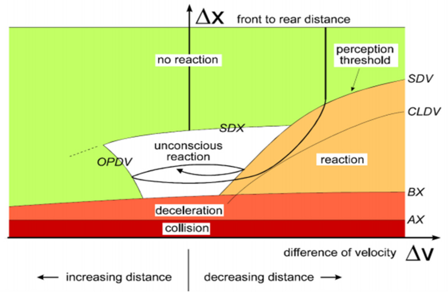
Vissim’s traffic flow model is a stochastic, time-step-based, microscopic model that treats driver-vehicle units as basic entities. The car-following model is based on the Wiedemann model. Driving behaviour in this model is divided into four states: free driving, approaching, following, and braking [
6,
15].
Figure 1 shows the driving behaviour reproduced in the model. The green colour is the situation when no other vehicle is in the distance needed for the reaction (that distance depends on the speed difference between two vehicles), the car is moving in the free flow with the velocity of its choice. When approaching the vehicle in front, after reaching the perception threshold (the moment when the driver notices the car in front), and the distance is small enough according to the difference in velocity, the following car starts to decelerate (light and dark orange colour). After reaching a similar speed and a proper distance, the following car speed oscillates randomly near the vehicle velocity in front of them, trying to adjust to a similar velocity and same distance (white colour) [
15].
Detailed driving behaviour is described with Wiedemann model parameters: Wiedemann 74, such as safety distances, lack of attention duration or lack of attention probability [
11]. Additionally, in Wiedemann 99: time distribution of the speed-dependent part of the desired safety distance, time of deceleration before reaching safe distance, influence of distance on speed oscillation, desired acceleration when starting from standstill [
15].
2.3. Relationship between Traffic Flow and Velocity
The relationship between traffic flow and velocity has been a research subject since the beginning of mass motorisation. First, a meaningful study of that topic was presented in the 13th Annual Meeting of the Highway Research Board in December 1933 by Greenshields [
16]. With the camera and chronometer in sight, the first measurements of density and speed were conducted. One of the most important results of the research was a fundamental diagram showing the relation between traffic volume (named in the research as “density”) and speed. That classic diagram is shown on
Figure 2.
On the diagram, there are two states of traffic visible. On the top is the state without congestion. With the growth in the traffic volume (D), there is a moderate decrease in the velocity, which continues to the point of reaching capacity. The other state, as seen on the bottom of the chart, is a low velocity and low traffic volume caused by congestion.
Primarily, fundamental diagrams of traffic flow were researched not for the urban streets but for highway traffic, establishing the relationship between traffic volume, velocity and capacity, level of service, etc. More advanced diagrams to use in urban areas were based on traffic density or a relationship with kinematic wave theory [
17,
18].
An alternative form of describing the relation between traffic flow and velocity is a volume–delay function. The volume–delay function (VDF) is an approximation of fundamental traffic phenomena such as gridlocks and spillbacks occurring in dynamic traffic models, for macroscopic, static models [
6,
19]. The VDF, unlike the fundamental diagram, is a function, containing a hypocritical part (where the traffic volume is below the capacity) and a hypercritical one.
One of the historically first and most popular formulations of VDFs are BPR functions, published in 1964 by the Bureau of Public Roads in USA [
4]. The other examples of VDFs can be Conical [
20] or Akcelik [
21] functions. Those function formulas are commonly used in macrosimulation models.
In the macroscopic model, the network is seen as a graph, where edges (links) (optionally nodes) are resistive. The resistance of the edges is described as a relationship between saturation grade (traffic volume to capacity ratio) and travel time (multiplied travel time of empty network), known as the volume–delay function. The volume–delay function is a nondescending, continuous, differentiable (with exception to the point sat = 1, where traffic volume is equal to capacity) function, usually calibrated based on assumptions or observations of the observed travel time and the corresponding volume data. [
22]. For unimpeded traffic flow, the result of the volume–delay function equals 1, meaning that vehicles travel with a free flow travel time. With the growth in traffic volume (vehicles per hour), the function values grow. When the traffic volume reaches capacity, the saturation grade equals 1. After crossing the capacity, the function starts to increase significantly. The example of the volume-delay function is shown in
Figure 3.
2.4. Macrosimulation Model and Traffic Assignment
Among the types of macrosimulation models according to the methods on which they were built, we considered a four-stage model. It consists of four steps: Trip generation, trip distribution, mode choice and traffic assignment [
24,
25].
Trip generation is the first stage in which spatial analysis is undertaken to determine the amount of trips going in and out of each homogenous area during the peak hour.
Trip distribution creates a matrix of trips between the origin and destination areas based on the gravity function, which determines the probability of a trip existing based on the distance or travel time.
Mode choice determines the amount of trips taken by every available means of transport, such as car, public transport, and bike. It is determined by functions defining the probability of choice of the specific means of transport according to distance, availability, and motivation (home-work, home-school etc.)
Traffic assignment sets the path for every trip generated, distributed and assigned to the transport mode in the previous stage. For the traffic assignment, Wardrop’s principle of user equilibrium is usually used [
26]. Its assumptions are that every user chooses the path with the lowest cost (cost is represented by travel time), and that the transport system aims to achieve equilibrium—the state when no vehicle can change the path to the other one, with a lower cost. However, for large networks, the simple user-equilibrium algorithm is relatively slow. Therefore, more time-efficient algorithms are used, based on the user-equilibrium rule, for example, the LUCE (Linear User Cost Equilibrium) algorithm, used in PTV Visum, which aims to be 10–100 times faster than other methods [
27]. The example of the traffic assignment is shown on
Figure 4.
Equilibrium methods require the iteration of traffic assignments, because the travel time on the link, the main factor to assign the trip to the path, depends on traffic flow, and thus on the amount of trips through the link in the form of volume–delay functions. Iterations are undertaken until the model reaches the equilibrium state.
In this research, only the last step of the four-step model is taken into the consideration, precisely, the traffic assignment reaction on the volume–delay functions existing on traffic-calmed roads.
3. Measurements and Building a Microsimulation Model
3.1. Methodology Overview
To produce the macrosimulation model, the vehicle movement was collected by unmanned aircraft with a video camera. Later, using video detection, the trajectories were produced with the help of machine learning. This allowed the extraction of the speed distributions of the vehicles, acceleration and braking—necessary parameters for the Vissim model, and speed profiles necessary for evaluation of the model. The overview is presented in
Figure 5. A more detailed methodology is presented in
Section 3.2,
Section 3.3,
Section 3.4 and
Section 3.5.
3.2. Location
The research area was Stachiewicza street in Kraków, Poland. There are speed cushions installed, two in each direction, allowing vehicles with a larger wheel gauge (such as buses) to pass them without slowdown. The street serves the role of one of the main connectors between the north-western and other districts, therefore carrying numerous and diversified traffic. Further, the direction “1” in this article means northbound, and “2” means southbound.
3.3. Video Data Collection
To provide coverage of the whole measured area, where a high point to place a camera was not present, an unmanned quadcopter (DJI Phantom IV) was used. Its coverage was 110 m of the street with an altitude of 80 m above ground level. The duration of the flight was approximately 25 min, which, after substracting the ascend and descend, left 15–20 min of traffic recording. The video parameters were: 1920 × 1080 pixels resolution and 40 frames per second.
The video footage was processed by the company DatafromSky [
29] to obtain the trajectories. The results of the processing delivered a graphical visualisation to watch in the DatafromSky viewer (see
Figure 6) and the csv file containing all trajectory data, such as: timestamp, coordinates, object ID, and object type (car, heavy vehicle, bus, bicycle, pedestrian).
3.4. Trajectory Analysis
The processing of the data acquired from the recordings was made as follows. First, the street visible in
Figure 6 was divided into measurement sections of 10 cm in length. Instantaneous velocities were identified in each section for every vehicle, with the division to vehicle classes, such as cars (standard and van), busses and heavy vehicles. Then, the sections were put together to create the speed charts showing the speed profiles of the analysed road, considering the velocity change on the speed cushions. For this measurement, 20 min of the recording was used, containing 192 vehicles: 165 cars, 18 vans, 3 heavy vehicles, and 6 busses. There were also 90 pedestrians detected, but these data were not used in this research. Charts of speed profiles are presented below in
Figure 7 and
Figure 8.
On the charts, speed profiles for the studied 107 m length of Stachiewicza Street can be seen. Speed cushions are indicated by violet dots on the top of the chart at 20 and 82 m along this section northbound, whereas southbound—on the 26th and 88th meter of the measured area. The minimum speed in each section is indicated with blue points. The decrease in the minimal velocity between the speed cushions (between 40th and 60th metre) shows the car stopping on the pedestrian crossing. The average velocity is represented with the green points—its decrease in the area of speed cushions is clearly visible. The red points marking the maximal speed show that there were vehicles which did not slow down on speed cushions, especially on the first one in the northbound direction.
3.5. Microsimulation Model
Building the microsimulation model started from preparing the speed distributions. Those were created according to the measured, cumulated frequencies for each vehicle type. There are two kinds of the speed distributions, corresponding to the two situations: near or away from the speed cushions. On the transfer between the speed distributions, the accelerations and braking were identified. In this model, there are two traffic directions, each on the separate link. There are two reduced speed areas in each link, representing the speed cushions. For every direction and for every reduced speed area, a separate speed distribution was inputted. Examples of the speed distributions are presented in
Figure 9.
In the vissim microsimulation model, the speed distributions, acceleration and deceleration data were inputted. Later, the simulation was undertaken for the traffic volume equal to that during the measurement, to check the calibration. To compare the simulated trajectory data with the measured ones, average speed profiles for all vehicles from the simulation were exported. The calibration was undertaken using the speed distributions when the traffic volume allows unimpeded traffic to correspond with the simulated velocities. Velocities in the simulation were adjusted to comply with the measurements. For the calibration of the speed profile shape, vehicles’ acceleration and braking were estimated. For the first direction of the Stachiewicza street (northbound), the correlation coefficient between the model and the measurement was equal to 0.79. The compared speed profiles are presented in
Figure 10.
For the second direction (southbound), the correlation coefficient was 0.71.
Figure 11 shows this comparison.
A correlation between measured and simulated speed profiles was clearly visible and acceptable. In case of needing correlation improvement and further calibration, the car-following model (Wiedemann) parameters can be adjusted or the link can be divided into more parts, with their own speed distributions, acceleration and breaking parameters.
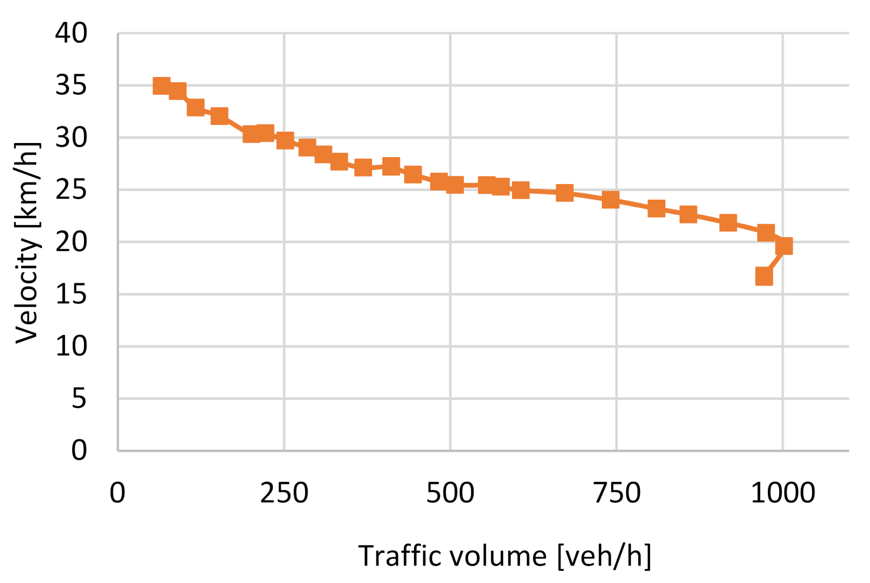
For the volume–delay function estimation, a variety of traffic volumes were simulated for both traffic-calmed and not-traffic-calmed links. To research the travel time in the traffic volumes exceeding the capacity, for the simulated link, another was added to accumulate the queues. Travel time (later used for the velocity calculation) is the travel time of the link with extensions (plus queue travel time if applicable) minus the travel time on extensions on the free flow. The initial result of that experiment was a relation between traffic volume [veh/h] and velocity [km/h]. This results in the chart shown in
Figure 12.
On
Figure 12, a descent in the speed with the traffic volume can be seen. At the point of reaching capacity, the velocity decreased with the maximal traffic volume, which created a relation complying with a fundamental diagram of traffic flow, where there are two results for velocity with the same traffic volume, depending on whether it is above or below capacity. To create a relation as a function, the traffic volume [veh/h] was replaced with the traffic density [veh/km] [
30]. In that case, after reaching the capacity, the density still increased with the decrease in the velocity. This is presented in
Figure 13.
The form of the travel times was calculated with the form corresponding to the volume–delay function presentation available in PTV Visum, meaning that the relationship between the saturation grade (density divided by the maximum traffic volume density) and the travel time is the t_0 (free flow travel time) multiplied by the rest of the function. In the macroscopic transport model of the city of Kraków, volume–delay functions were estimated using the BPR2 volume–delay functions shape (see Formula (1)):
Formula (1). BPR volume–delay function, source: [
4]
where:
t0—free flow travel time (for the following speeds: with traffic calming: 28 km/h, without traffic calming: 30 km/h);
a, b, b′—parameters of the function;
sat—saturation grade (q/qmax).
Estimating the function parameters for the best fit was made using the squared difference minimisation. Parameters’ values are shown in
Table 1.
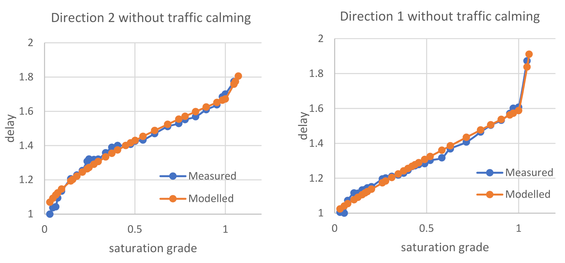
The fitting of the function had a high correlation coefficient, in every case above 0.9. The comparison of the empirical relation with the function fitting can be seen in
Figure 14.
4. Experiment
In this experiment, a “toy network” of two links of the same length was constructed, connecting a common origin and a destination. The links differed in the volume–delay function defined for them—one with, the other without traffic calming; thus, the travel time is as seen in Formulas (2) and (3):
Formula (2). Travel time with traffic calming. Source: own, based on: [
4]
Formula (3). Travel time without traffic calming
In the experiment, we researched a situation when our toy network is in the state of equilibrium. That means, for every user, the travel time is the same twtc = twotc. In that case, the traffic volume would be different for each link, which is written as qwtc: traffic volume for a link with the traffic calming and the remaining traffic (on the link without traffic calming): qtot − qwtc, where the total traffic flow is described by qtot. The traffic assignment on this simple network was calculated by solving the equation given in Formula (4): twtc = twotc.
Formula (4): The equation of the model
Calculations of the traffic assignment were made with the help of Microsoft Excel’s Solver together with the use of macros to automate the process of simulating various traffic volumes, and these were then confirmed with PTV Visum software (using the equilibrium traffic assignment for the aforementioned model). A graphical description of the model can be seen in
Figure 15. There are two pictures with each of them containing different total traffic (
qtot): on the left: 500 veh/h, on the right—3000 veh/h. For this model, the BPR function values of Direction 2 stated in
Table 1 are used—the top with traffic calming (
wtc) and the bottom without traffic calming (
wotc).
5. Results
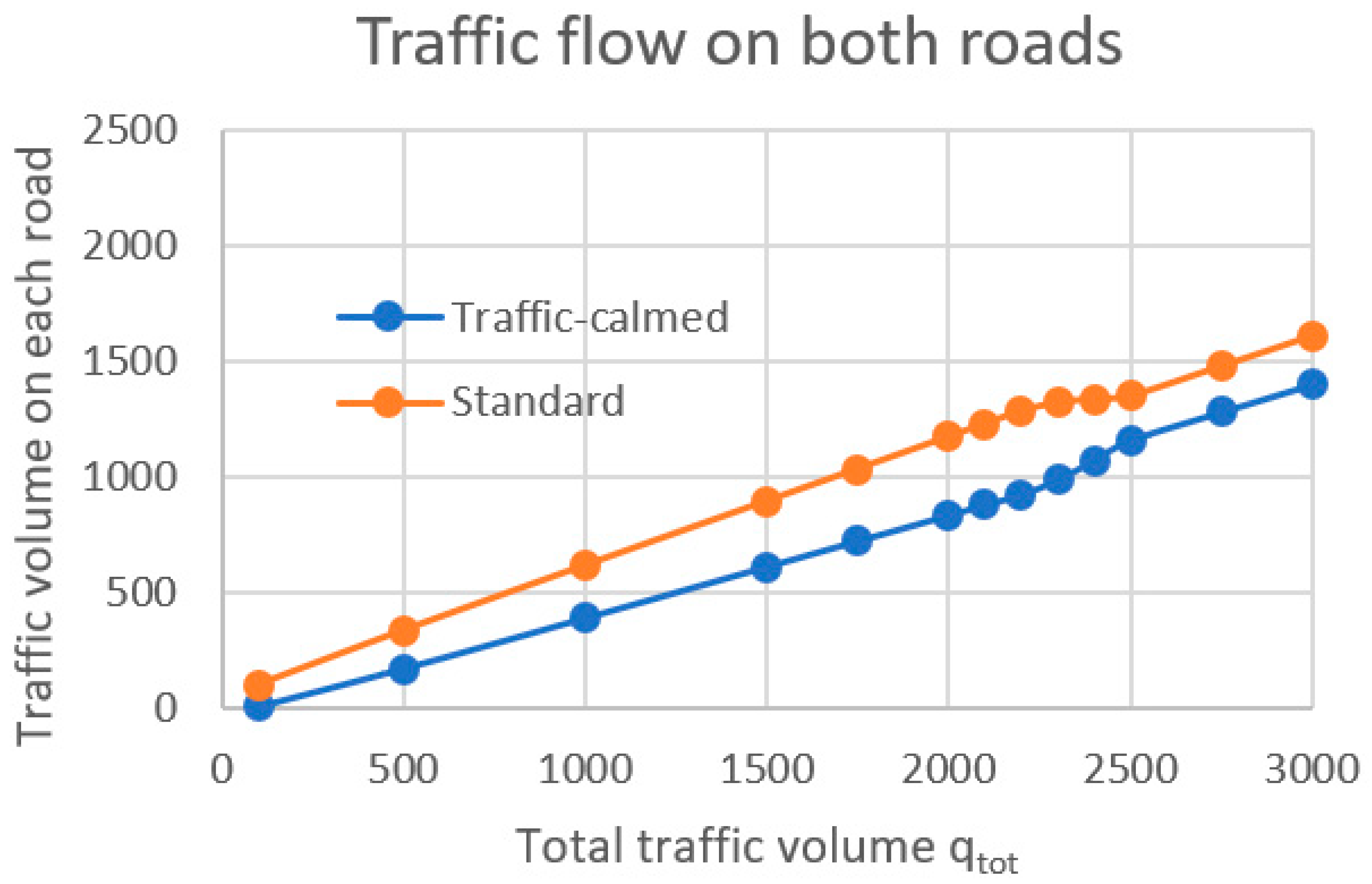
As a result of the experiment, a chart showing the relation between the total traffic volume (q
tot) and the traffic volume on each link was created. The results are shown in
Figure 16.
For a better interpretation of the above chart, it was shown (on
Figure 17) as a difference in traffic volume between each link.
The phenomena presented in the chart can be divided into three phases, depending on the state of the network:
Both links are below capacity. On the empty street, the speed is lower on the traffic-calmed road (because of the slowdown caused by speed cushions) than on the road without traffic calming. No or a little slowdown is caused by a high traffic volume. More vehicles choose the standard road. qtot ≤ 2200 veh/h.
Because more vehicles choose the standard road, it reaches capacity earlier (despite the capacity being higher than the other link) and causes congestion; thus, drivers choose an alternative road through a traffic-calmed one, which is still under capacity. 2200 < qtot ≤ 2500 veh/h.
Traffic-calmed road exceeds capacity, as well as standard road; more vehicles choose the standard road, with higher speeds during congestion. qtot > 2500 veh/h.
The difference between the traffic volumes on links with the aforementioned volume–delay functions in relation to total traffic volume was modelled as a polynomial function shown in Formula (4):
. Function parameters are presented in
Table 2.
Formula (5). Estimation function formula
The results of the function fitting have been presented in
Figure 18.
Comparison with the Results of the Current Solutions
Currently, in existing macroscopic urban models, in most of the cases, there is no modelling of the volume–delay functions for traffic-calmed roads. Either for roads with small traffic (where traffic-calmed ones often belong) are no volume–delay functions defined (meaning that the travel time is not dependent on the traffic volume) or a volume–delay function is standard for the whole link type. It is considered that the traffic on the toy network of two links would be simulated as the same for both types of links unless there is no differentiation in the free flow velocity. However, when that v
0 velocity is different, in the case of a constant volume–delay function, there will be no traffic on the traffic-calmed road, because it is always slower than the other one. In the case of using the same volume–delay function, together with a different v
0 velocity, which is a proper solution in existing models, the result will be as in the
Figure 19.
The difference between traffic volumes is shown on
Figure 20.
Comparing the last two charts with
Figure 19 and
Figure 20, we can see similarities such as the aforementioned three stages of traffic and similar values below the capacity. This is a result of a similar shape of the volume–delay functions for a standard and traffic-calmed road below capacity. However, the difference in the shape of the volume–delay functions above the capacity corresponds with a different traffic assignment behaviour. When we have different VDFs, the difference grows exponentially; otherwise, it grows linearly.
The described behaviour should occur in this specific case, but it is also the universal reaction of the macroscopic model for the change in the volume–delay functions. The experiment and comparison with the other possible methods show that applying volume–delay functions dedicated for the traffic-calmed areas gives other, possibly more precise traffic assignment results.
6. Summary
The aim of the article was to show the method of modelling a volume–delay function through video-detecting trajectories and microscopic modelling, and to use those functions to research traffic assignment. For the researched street, using this method, volume–delay functions’ parameters were estimated. That led to the analysis of the traffic assignment on the “toy network” using the aforementioned functions. It was shown that a traffic-calmed road attracts less traffic compared with that without. Lastly, the article showed that using different volume–delay functions for describing traffic calming for macroscopic modelling makes a difference in a traffic assignment results. For the comparison and discussion with the other research in this field, similar research using methodology used in this was not found. The results of this paper can help in understanding a traffic assignment of traffic-calmed roads. For further research, other traffic-calming measures than speed cushions can be used. This would allow a comparison of various traffic-calming measures regarding the influence of the traffic calming.
Author Contributions
Conceptualization: J.P., M.R. and A.S.; Methodology: J.P. and M.H.; Software: J.P. and M.H.; Validation: J.P.; Formal analysis: J.P. and M.H.; Investigation: J.P., M.R., A.S. and M.H.; Data curation: J.P. and M.H.; Writing—original draft preparation: J.P.; Writing—review and editing: M.R. and A.S.; Visualisation: J.P.; Supervision: M.R. and A.S. All authors have read and agreed to the published version of the manuscript.
Funding
This research received no external funding.
Institutional Review Board Statement
This study did not involve humans or animals.
Informed Consent Statement
Not applicable.
Data Availability Statement
Not applicable.
Acknowledgments
The authors would like to thank the Saxon State Ministry of Science and Art, represented by the State of Saxony, for their partial funding of the research project “Applied research in the future field of digital communication” (diKo19/diKo20), under which this research was conducted.
Conflicts of Interest
The authors declare no conflict of interest.
References
- ITE/FHWA. Traffic Calming: State of the Practice; Federal Highway Administration: Washington, DC, USA; Institute for Transportation Engineers: Washington, DC, USA, 1999. [Google Scholar]
- Brindle, R.E. Australia’s Contribution to Traffic Calming; Pearson: London, UK; PTRC: Kernersville, NC, USA, 1992. [Google Scholar]
- Bureau of Public Roads. Traffic Assignment Manual; Department of Commerce, Urban Planning Division: Washington, DC, USA, 1964. [Google Scholar]
- GPS Accuracy. 2018. Available online: https://www.gps.gov/systems/gps/performance/accuracy/ (accessed on 18 March 2018).
- Barbosa, H.M. Impacts of Traffic Calming Measures on Speeds on Urban Roads; University of Leeds: Leeds, UK, 1995. [Google Scholar]
- Kucharski, R. Makroskopowy Model Przepływu Ruchu w Sieci Drugiego Rzędu–Alternatywny Opis Stanu Sieci. In Proceedings of the Poznań-Rosnówko, Problemy Komunikacyjne Miast w Warunkach Zatłoczenia Motoryzacyjnego, Poznań-Rosnówko, Poland, 19–21 June 2013. [Google Scholar]
- Pipes, L.A. An operational analysis of traffic dynamics. J. Appl. Phys. 1953, 24, 274–281. [Google Scholar] [CrossRef]
- Forbes, T.W.; Zagorski, H.J.; Holshouser, E.L.; Deterline, W.A. Measurement of driver reactions to tunnel conditions. In Proceedings of the Highway Research Board, Washington, DC, USA, 6–10 January 1958; Volume 37. [Google Scholar]
- Gazis, D.C.; Herman, R.; Rothery, R.W. Nonlinear follow-the-leader models of traffic flow. Oper. Res. 1961, 9, 437–599. [Google Scholar] [CrossRef]
- Newell, G.F. Nonlinear effects in the dynamics of car following. Oper. Res. 1961, 9, 209–229. [Google Scholar] [CrossRef]
- Wiedemann, R. Simulation des Straßenverkehrsflusses, 1974th ed.; Institut für Verkehrswesen: Karlsruhe, Germany, 1974; Available online: https://trid.trb.org/view/596235 (accessed on 19 June 2021).
- Bando, M.; Hasebe, K.; Nakanishi, K.; Nakayama, A. Analysis of optimal velocity model with explicit delay. Phys. Rev. E 1998, 58, 5429–5435. [Google Scholar] [CrossRef] [Green Version]
- Treiber, M.; Kesting, A. Microscopic calibration and validation of car-following models—A systematic approach. Procedia Soc. Behav. Sci. 2013, 80, 922–939. [Google Scholar] [CrossRef] [Green Version]
- Raju, N.; Arkatkar, S.; Joshi, G. Evaluating performance of selected vehicle following models using trajectory data under mixed traffic conditions. J. Intell. Trans.Sys. 2020, 24, 617–634. [Google Scholar] [CrossRef]
- PTV-AG. PTV VISSIM 9 User Manual; PTV-AG: Karlsruhe, Germany, 2017. [Google Scholar]
- Greenshields, B. A Study of Traffic Capacity. Highw. Res. Board Proc. 1935, 14, 448–477. [Google Scholar]
- Daganzo, G. An analytical approximation for the macroscopic fundamental diagram of urban traffic. Transp. Res. Part B Methodol. 2008, 42, 771–781. [Google Scholar] [CrossRef]
- Helbing, D. Derivation of a fundamental diagram for urban traffic flow. Eur. Phys. J. B 2008, 70, 229–241. [Google Scholar] [CrossRef] [Green Version]
- Kucharski, R.; Drabicki, A. Estimating Macroscopic Volume Delay Functions with the Traffic Density Derived from Measured Speeds and Flows. J. Adv. Trans. 2017. [Google Scholar] [CrossRef]
- Spiess, H. Technical note—Conical volume-delay functions. Trans. Sci. 1990, 24, 153–158. [Google Scholar] [CrossRef] [Green Version]
- Akcelik, R. Travel time functions for transport planning purposes: Davidson’s function, its time dependent form and alternative travel time function. Aust. Road Res. 1991, 21, 49–59. [Google Scholar]
- Petrik, O.; Filipe, M.; de Abreu e Silva, J. The Influence of the Volume–Delay Function on Uncertainty Assessment for a Four-Step Model. Adv. Intell. Syst. Comput. 2014, 262, 293–306. [Google Scholar]
- Cascetta, E. Transportation Systems Engineering: Theory and Methods, 49th ed.; Springer Science: Berlin, Germany, 2013. [Google Scholar] [CrossRef]
- Manheim, M.L. Fundamentals of Transportation Systems Analysis; MIT Press: Cambridge, MA, USA, 1979. [Google Scholar]
- Florian, M.; Gaudry, M.; Lardinois, C. A two-dimensional framework for the understanding of transportation planning models. Transp. Res. B 1988, 22, 411–419. [Google Scholar] [CrossRef]
- Wardrop, J.G. Some Theoretical Aspects of Road Traffic Research. Proc. Inst. Civil Eng. 1952, 1, 325–362. [Google Scholar] [CrossRef]
- Gentile, G.; Noekel, K. Linear User Cost Equilibrium: The new algorithm for traffic assignment in VISUM. In Conference Papers 2009; AET: Noordwijkerhout, The Netherlands, 2009. [Google Scholar]
- Szarata’s Team. Badania Zachowań Komunikacyjnych Mieszkańców Krakowskiego Obszaru Metropolitarnego; Kraków: Technical Report. 2014. Available online: https://www.bip.krakow.pl/?sub_dok_id=96964 (accessed on 19 June 2021).
- Available online: http://datafromsky.com/ (accessed on 15 May 2019).
- Richter, M.; Paszkowski, J. Modelling driver behaviour in traffic-calmed areas. Czas. Tech. 2018, 8, 111–124. [Google Scholar]
Figure 1.
States of PTV Vissim model, source: PTV Vissim 9 manual [
15].
Figure 1.
States of PTV Vissim model, source: PTV Vissim 9 manual [
15].
Figure 2.
Greenshield’s fundamental diagram of traffic flow, source: [
16].
Figure 2.
Greenshield’s fundamental diagram of traffic flow, source: [
16].
Figure 3.
Example of volume–delay functions, source: [
23].
Figure 3.
Example of volume–delay functions, source: [
23].
Figure 4.
Example of traffic assignment for the city of Kraków. Source: [
28].
Figure 4.
Example of traffic assignment for the city of Kraków. Source: [
28].
Figure 5.
Methodology diagram. Source: own.
Figure 5.
Methodology diagram. Source: own.
Figure 6.
DatafromSky viewer software screenshot with car detection and trajectory data displayed (source: own).
Figure 6.
DatafromSky viewer software screenshot with car detection and trajectory data displayed (source: own).
Figure 7.
Speed profile for Stachiewicza street, direction northbound (source: own).
Figure 7.
Speed profile for Stachiewicza street, direction northbound (source: own).
Figure 8.
Speed profile for Stachiewicza street, direction southbound (source: own).
Figure 8.
Speed profile for Stachiewicza street, direction southbound (source: own).
Figure 9.
Car speed distributions for the link, direction southbound (orange) and its second speed cushion (blue), source: own.
Figure 9.
Car speed distributions for the link, direction southbound (orange) and its second speed cushion (blue), source: own.
Figure 10.
Comparison of speed profiles on the measured street section, heading northbound, source: own.
Figure 10.
Comparison of speed profiles on the measured street section, heading northbound, source: own.
Figure 11.
Comparison of speed profiles on the measured street section, heading southbound, source: own.
Figure 11.
Comparison of speed profiles on the measured street section, heading southbound, source: own.
Figure 12.
Traffic volume–speed relation, source: own.
Figure 12.
Traffic volume–speed relation, source: own.
Figure 13.
Traffic density–speed relation, source: own.
Figure 13.
Traffic density–speed relation, source: own.
Figure 14.
Fitting of the volume–delay functions, source: own.
Figure 14.
Fitting of the volume–delay functions, source: own.
Figure 15.
Example results of the traffic assignment, source: own.
Figure 15.
Example results of the traffic assignment, source: own.
Figure 16.
Traffic flow on both roads according to the total traffic volume, source: own.
Figure 16.
Traffic flow on both roads according to the total traffic volume, source: own.
Figure 17.
Difference in traffic flow on each link, source: own.
Figure 17.
Difference in traffic flow on each link, source: own.
Figure 18.
Fitting of the function, source: own.
Figure 18.
Fitting of the function, source: own.
Figure 19.
Traffic flow on both roads with the same volume–delay function and different v0 velocities, source: own.
Figure 19.
Traffic flow on both roads with the same volume–delay function and different v0 velocities, source: own.
Figure 20.
Difference in traffic volume between links with the same volume–delay function and different v0 velocities, source: own.
Figure 20.
Difference in traffic volume between links with the same volume–delay function and different v0 velocities, source: own.
Table 1.
Function parameter values.
Table 1.
Function parameter values.
| Number of Function | Direction 1 with Traffic Calming | Direction 2 with Traffic Calming | Direction 1 without Traffic Calming | Direction 2 without Traffic Calming |
|---|
| a= | 0.641359 | 0.758637 | 0.527618 | 0.611864 |
| b= | 0.738809 | 0.643984 | 0.905478 | 0.646525 |
| b′= | 6.760153 | 5.292947 | 7.080322 | 2.591875 |
| qmax | 1068 | 1044 | 1308 | 1158 |
Table 2.
Function parameters.
Table 2.
Function parameters.
| | a | b | c |
|---|
| 1. qtot ≤ 2200 veh/h | 1.75075 | 44.77371 | 0.00049 |
| 2. 2200 < qtot ≤ 2500 veh/h | 1.06087 | 1203.81532 | −0.23048 |
| 3. qtot > 2500 veh/h | 2.93892 | 0.141 × 10⁻¹² | 0.259 × 10⁻⁸ |
| Publisher’s Note: MDPI stays neutral with regard to jurisdictional claims in published maps and institutional affiliations. |
© 2021 by the authors. Licensee MDPI, Basel, Switzerland. This article is an open access article distributed under the terms and conditions of the Creative Commons Attribution (CC BY) license (https://creativecommons.org/licenses/by/4.0/).


