Demand-Side Optimal Sizing of a Solar Energy–Biomass Hybrid System for Isolated Greenhouse Environments: Methodology and Application Example

Abstract

The water–energy–food nexus has captured the attention of many researchers and policy makers for the potential synergies between those sectors, including the development of self-sustainable solutions for agriculture systems. This paper poses a novel design approach aimed at balancing the trade-off between the computational burden and accuracy of the results. The method is based on the combination of static energy hub models of the system components and rule-based control to simulate the operational costs over a one-year period as well as a global optimization algorithm that provides, from those results, a design that maximizes the solar energy contribution. The presented real-world case study is based on an isolated greenhouse, whose water needs are met due to a desalination facility, both acting as heat consumers, as well as a solar thermal field and a biomass boiler that cover the demand. Considering the Almerian climate and 1 ha of tomato crops with two growing seasons, the optimal design parameters were determined to be (with a solar fraction of 16% and a biomass fraction of 84%): 266 m${}^2$ for the incident area of the solar field, 425 kWh for the thermal storage system, and 4234 kW for the biomass-generated power. The Levelized Cost of Heat (LCOH) values obtained for the solar field and biomass boiler were 0.035 and 0.078 €/kWh, respectively, and the discounted payback period also confirmed the profitability of the plant for fuel prices over 0.05 €/kWh. Thus, the proposed algorithm is useful as an innovative decision-making tool for farmers, for whom the burden of transitioning to sustainable farming systems might increase in the near future.

1. Introduction

The growth of the world population, together with other environmental factors, such as climate change, are putting great pressure on the resources used to provide essential commodities for humankind. This is particularly noticeable for the water and food supply as well as others, such as energy, which is required in any kind of developed society that seeks to ensure human welfare. The magnitude of the problem increases if the nexus between these resources is taken into account. Water is fundamental for the agricultural sector, the main source of food, whereas energy is required to maintain suitable conditions for crop yield, as well as to transport and process food products, and in many any other links of the supply chain. In addition, energy determines the efficiency and effectiveness of water use, which is fundamental in creating the conditions for sustainable food production. This relationship has given rise to the so-called “water–energy–food (WEF) nexus”, which has been recognized as one of the crucial problems that humanity must face for proper and sustainable development [1,2].

Currently, the agriculture industry is the world’s main water consumer, approximately utilizing 80% of the total consumption (with territorial variations due to economic development and climatology [3]); however, this figure is expected to increase as the surface area used for irrigated crops does, by 1.3% per year according to the current trend [4]. This increase in water consumption can compromise the sustainability of the agricultural system in arid or semi-arid regions, such as the Mediterranean basin, causing severe economic problems as many of these places base their economy on this sector. Indeed, not only economic upheaval can arise but there will also be environmental degradation and a true social crisis as a consequence.

For these reasons, the use of desalination technologies has emerged as one of the most promising solutions to expand natural water reserves and mitigate water deficits in agriculture ecosystems [5]. However, massive and indiscriminate use of this technology can lead to cost overruns and serious environmental problems, since, currently, most of the energy requirements for these facilities come from on-grid electricity obtained by conventional sources, such as fossil fuels, and only around 1% of the total worldwide desalination facilities are powered on a sustainable way through renewable sources [6].

To deal with the aforementioned challenges, it is necessary to promote the use of alternative desalination technologies that allow a direct coupling with renewable energies and that can adapt their production to the water demand of agricultural holdings to avoid cost overruns in the desalinated water, which is claimed to be one of the main problems preventing the adequate use of desalinated water in agriculture systems in some target regions [7].

Membrane Distillation (MD) technology is an alternative desalination method that presents a wide variety of advantages to be used in agriculture environments [8]. This method consists of a thermally driven desalination technique that can deal with low–medium water needs and operate in a discontinuous and intermittent mode [9], which is consistent with the needs of small- to medium-sized agricultural settings as demonstrated in our previous work [10]. In addition, this technique can produce desalinated water from different sources, such as sea or brackish water and can treat even high salinity solutions reaching zero-liquid discharges, thus, avoiding the environmental problem that brines can produce [11]. Nevertheless, the main interest lies in its low operating temperature, which allows the MD modules to be easily coupled with low-enthalpy energy sources, such as low-grade solar thermal energy or waste heat [12]. Hence, this technology is currently in the spotlight, as an adequate alternative to be included in sustainable agricultural systems where renewable energies play a major role. Such is the case of greenhouse crops, for which there is a growing trend to use renewable or neutral emissions sources to supply heat, among other purposes [13].

Although greenhouses are normally placed in locations with favourable conditions to keep the operational costs as low as possible, most of them require heat for frost prevention or for maintaining an appropriate crop temperature over winter. Despite this, only a small number of growers can afford auxiliary heaters due to their relatively high cost, and those who can, typically install combustion systems based on natural gas or diesel oil, which worsens the problem of environmental pollution [14]. It is, then, not surprising that solar heating systems are attracting increased attention to respond to the imperative for minimum emissions and sustainable development [15]. Moreover, this energy source becomes particularly economically profitable in isolated or rural areas, where the cost of the aforementioned conventional energy carriers can significantly increase due to transport issues. In this context of self-sufficient environments powered by renewable energies, greenhouses, and thermal desalination technologies (i.e., MD) can emerge, providing a unique solution to address the water–energy–food nexus [16].

Different studies have evaluated the feasibility and performance of solar thermal systems for heat supply in greenhouses. For instance, in [17], the authors analysed the operation of flat-plate collectors in greenhouse environments and concluded that this technology is a profitable solution with less environmental impact than conventional systems. A similar study was carried out in [18], where the profitability of solar thermal systems in comparison with conventional heating systems, such as heat pumps, was demonstrated as well.

In [19], the authors demonstrated how the cost of a heating system could be reduced up to 25% by including solar thermal technology. However, in all of the above-mentioned references, the authors stated that, even with thermal storage systems, other backup devices were needed to cope with the whole demand of the greenhouse because of its irregular behaviour linked to the availability of solar irradiance. Therefore, in the line with the ideas presented in [13], a mixed hybrid heating system based on solar-biomass energy can be proven to be an efficient solution to provide all the necessary energy to these environments. This was also stated in [20], where the authors researched the use of such hybrid systems for heat provision in rural locations. The use of biomass energy is particularly suitable since agriculture environments present a unique opportunity to reuse part of their waste as biomass, thus, creating added value and contributing to a circular economy [21].

Additionally, food waste, which is tightly linked with energy challenges [22] and is intense in agricultural production [23], can also be used in the above-mentioned context due to its potential to produce valuable fuels [24,25]. However, in order to exploit all the advantages that solar energy–biomass hybrid systems can offer and to make them profitable, further design methods that include economical, technical, and environmental aspects, and that take into account, in an integrated way, the optimization and operation of the system are nevertheless yet to be addressed, as they have barely been developed in the literature thus far.

To the best of authors’ knowledge, the most complete study dealing with the above issue was presented in [26], where an optimization method to design hybrid systems based on solar energy and biomass for supplying heat to industrial processes was proposed. In that study, the authors formulated an optimization problem based on a weighted-sum objective function that attempted to maximize the solar energy contribution while minimizing the net energy balance of the complete system, which is tackled through a dynamic model programmed in TRNSYS and MATLAB. Even though the proposed method considers the variability on the demand profile—a basic requirement for the correct design of these systems—the use of a dynamic model considerably penalized the computational burden when solving the problem. In fact, the authors designed the system considering only one week of data. Such a high computational burden discourages the use of the proposed method for more complex and accurate analyses—for example, with very heterogeneous demands or longer periods of data, of at least one year, that include seasonality—unless a wide enough parallel computing network is employed. Furthermore, considering the objective function as a weighted sum, which defines a multi-objective optimization problem, requires carrying out numerous tests to tune the weighting factors until reaching the desired solution, and therefore delaying and further complicating the design process.

According to the above literature review, the main novelty of the present article lies in the development of a demand-side optimal design method for hybrid systems that allows users to perform an optimal dimensioning considering a heterogeneous demand over the year, and the exemplification of this via an actual system representative of the WEF nexus. In this sense, the main contributions can be summarized as follows:

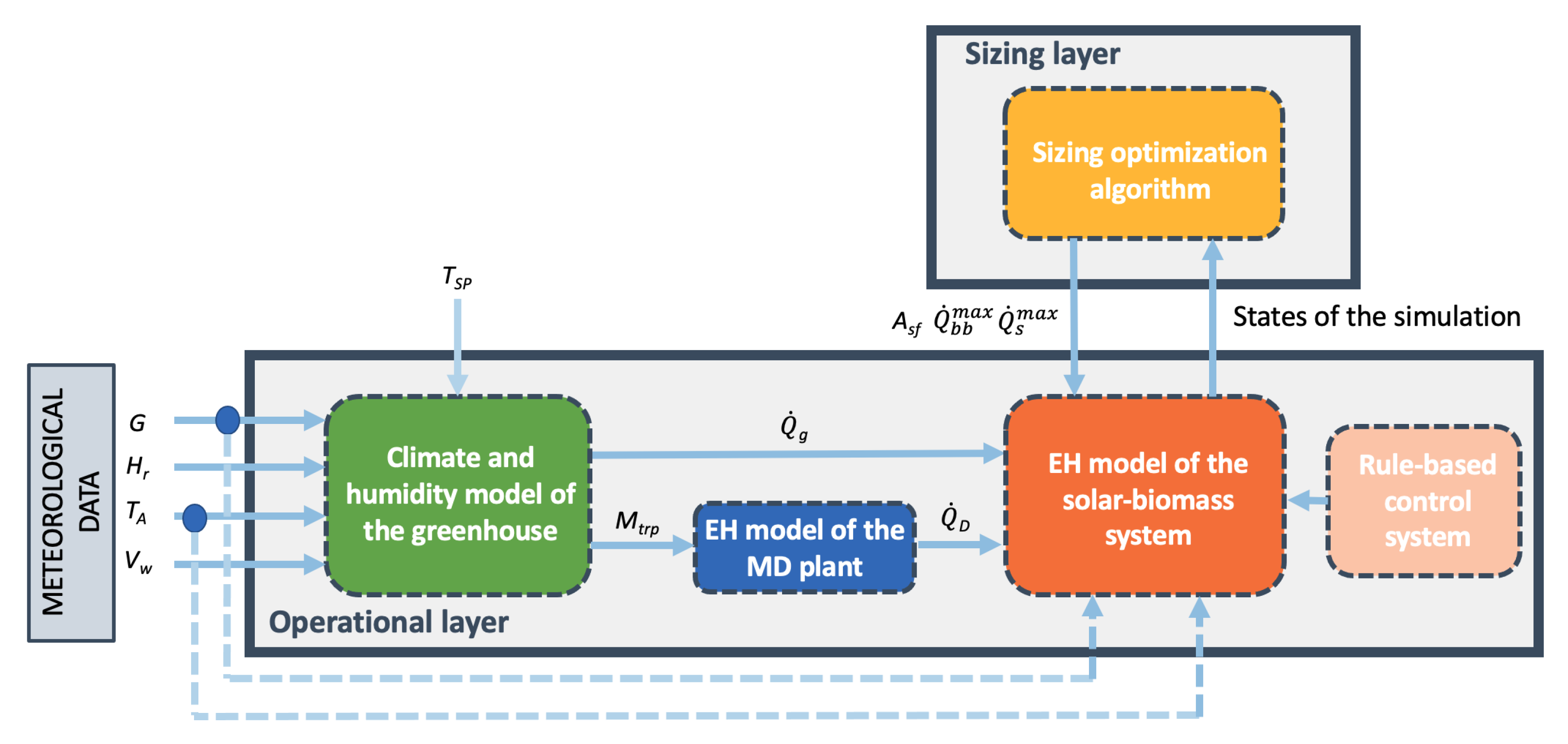
• A demand-side optimal sizing algorithm composed of two layers is presented. The upper layer performs the design, based on a global optimization algorithm that attempts to maximize the solar energy contribution in the hybrid system. Unlike the approach presented in [26], the optimization problem is formulated as a single-objective problem with an operational constraint that prevents the key elements, such as the solar field, from being oversized. The approach itself facilitates its applicability since no setting parameters need to be tuned.
  On the other hand, the lower layer is responsible for evaluating the operation of the hybrid system from the sizing parameters provided by the upper layer and sending the results back to the same one; hence, they are in continuous communication until the optimization algorithm converges to the global solution of the problem. Therefore, the algorithm offers a solution that integrates both the operation of the system over the period of time considered and the optimal design of its sizing parameters.
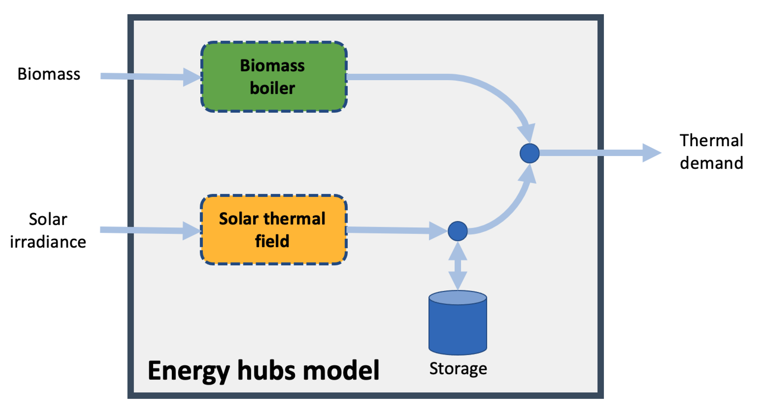
• The Energy Hubs (EH) [27] approach is proposed to link the two aforementioned layers. This broad methodology allows one to build a model that represents energy and mass balances between certain input resources that can be converted into other output resources. Each component of the system is usually characterized by static or time-variant conversion factors, thus, considerably decreasing the computational burden of the problem. A complete EH model for these kinds of systems is proposed, and the way in which these models are related to the sizing parameters provided by the optimization technique is depicted. This type of modelling methodology is justified as long as an effective low-level controller is implemented in the systems under study, which was addressed in previous studies [28,29] for the solar thermal field and biomass system, respectively.
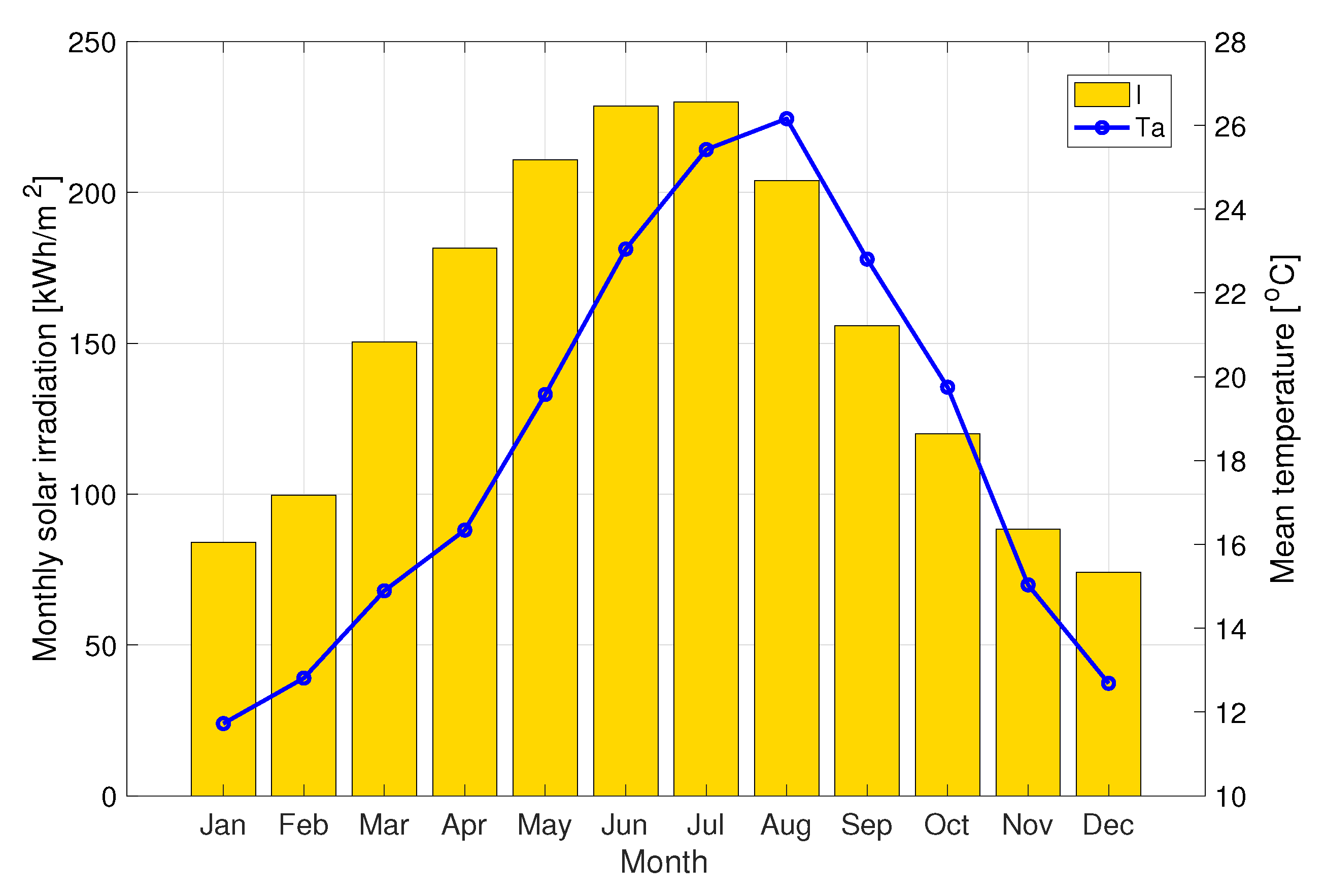
• A case study in the province of Almería (Southeast Spain) is presented to illustrate the performance of the proposed methodology. In this case study, a full year of data on an hourly basis was used for design. The results obtained are analysed in operating and economic terms demonstrating and validating the good performance of the proposed methodology. The province of Almería is a region of special interest since, on the one hand, its main economic driving force is agriculture based on greenhouse crop production [30,31], and, on the other, it has a wide availability of solar energy, which makes the implementation of solar-based technologies viable.
  In addition, this province is the perfect illustration of the relevance of the WEF nexus in the situation where there are trade-offs between (1) the production of high-quality products that supply a large part of Europe with healthy food, (2) a development model that has turned the poorest province in Spain into a reasonably equitable cooperative agricultural model, and (3) huge stress on the water resources and aquifers as well as problems with dealing with nitrate directives and controlling greenhouse expansion. Thus, the solution offered by this paper is part of the puzzle of the transitioning agricultural systems into more sustainable pathways.

The paper is arranged as follows. Section 2 is devoted to a description of the hybrid system and the formulation of the EH model. Section 3 presents the development of the proposed design optimization method, discussing how the demand is calculated, how the hybrid facility is operated, and posing the optimization problem. Section 4 shows and discusses the results obtained in the case study. Finally, Section 5 summarizes the main findings of this study.

2. Hybrid Plant Description and Modeling

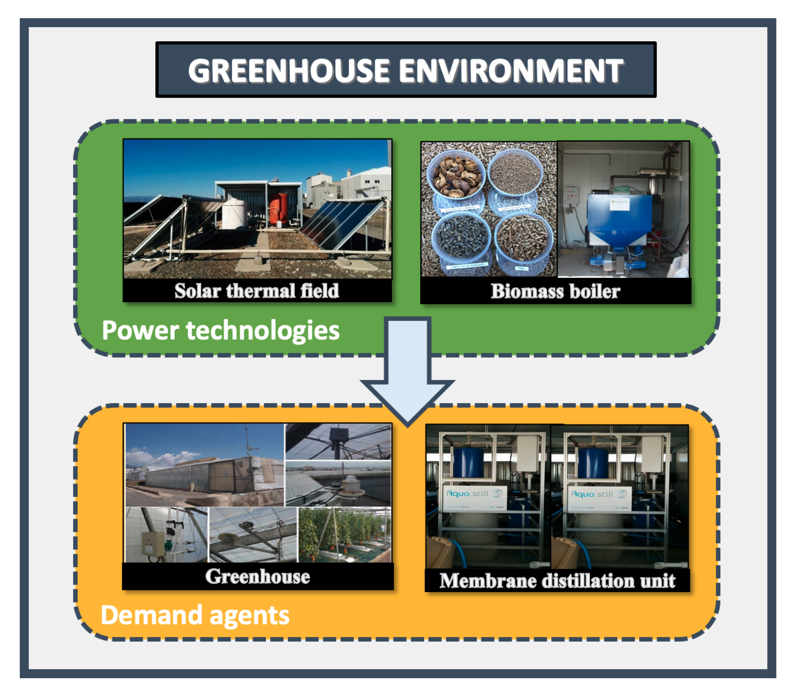
2.1. Plant Description

In this article, a hybrid network composed of a solar thermal field and a biomass boiler aims to cover the demands of an isolated greenhouse environment that is located in a coastal area. Thermal energy is required to maintain the desired temperature range for the crops and to power a thermal desalination unit in charge of providing irrigation water. The layout of this environment is presented in Figure 1, and this is based on different real facilities located in Almería (Southeast of Spain).

This real representative environment allows us to directly address actual production concerns and experiences, which is essential to demonstrate the adequacy of the proposed method and the applicability of the obtained results. Nevertheless, it should be remarked that these facilities are exclusively used to determine the key parameters for the EH modelling of the system, such as efficiency or conversion factors, and to determine the heat demand of the greenhouse. However, they will be appropriately scaled through the design technique proposed in this article for the case study addressed as described in Section 4.

For the solar thermal field and the thermal desalination facility, the solar membrane distillation pilot plant located at Plataforma Solar de Almería (PSA, www.psa.es (accessed on 9 June 2021)) is used as a reference. The solar thermal field consists of two rows of five flat-plate collectors: Solaris CP1–Nova by Solaris Energía Solar SA, with an area of 2 m${}^2$ each, so that the total area of the solar field is 20 m${}^2$. Its total nominal capacity is 7 kW_th at 90 °C, and its output is connected to a thermal storage tank of 1.5 m${}^3$ that is used as an energy buffer. The thermal desalination unit uses a commercial air-gap MD module manufactured by Aquastill. This module has a total effective membrane area of 24 m${}^2$, providing a maximum distillate production of around 30 L/h under the best operating conditions [32]. Further information about this pilot plant can be found elsewhere [33].

The greenhouse and the biomass boiler are located at the Experimental Station of the Cajamar Foundation, also in the province of Almería but 40 km from the PSA. The first one is an Almería-type greenhouse (E–W orientation), with a total area of 821 m${}^2$, 616 m${}^2$ of which are available for cultivation purposes. The cover is made of polyethylene, and the greenhouse is equipped with an automatic ventilation system, incorporating side windows on the south and north walls. On the other hand, the Missouri 150,000 multi-fuel boiler (normally fed with biomass) is available to meet the crop’s necessities. A more extensive description of this facility can be found in [29].

2.2. Model of the Hybrid System

Although the hybrid system is based on the aforementioned real plants, the main idea behind this work is to determine the optimal size of the solar field, storage tank, and biomass boiler. For this aim, these elements were modelled through the EH methodology, since it allows one to obtain a direct relationship between the operation of the different subsystems and the main design parameters that determine their size, i.e., the total area of the solar field, capacity of the thermal storage tank, and maximum power of the biomass boiler.

The schematic diagram of the EH model is presented in Figure 2, where each of the components is modelled through an input port, related to any kind of energy carrier; a conversion factor, for modelling the conversion of resources or energy; and an output port, which represents the demand of any kind of energy [27]. In the case of the biomass boiler, the input is the amount of biomass burned whereas the output is the thermal power provided to the demand agents. In the solar thermal field, the input is the solar irradiance, whereas the output is the thermal power delivered to the same agents.

Regarding the conversion factors, the biomass boiler’s can be calculated based on the boiler’s overall efficiency (${\eta }_b$) and the Lower Heating Value (LHV) of the biomass. This factor (${\eta }_{BB}$) relates the biomass flow (${\dot{m}}_B$) provided to the system with the heat flux generated by the biomass-generated power (${\dot{Q}}_{BB}$) [34]:

$$\frac{{\dot{Q}}_{BB}\left(k\right)}{{\dot{m}}_B\left(k\right)}={\eta }_{BB}={\eta }_b·LHV,$$

(1)

where k represents a discrete instant of time. In addition, the output of this equation is limited according to the maximum power that the biomass system can provide:

$$0\le {\dot{Q}}_{BB}\left(k\right)\le {\dot{Q}}_{BB}^{max}.$$

(2)

In this constraint, the parameter ${\dot{Q}}_{BB}^{max}$ will be computed by the optimization algorithm responsible for determining the optimal size of the system.

In the case of the solar field, the conversion factor (${\eta }_{sf}$) that relates the radiant power received by the solar field (I) to the thermal power generated (${\dot{Q}}_{sf}$) can be calculated according to the efficiency of the solar collectors [35] as:

$$\frac{{\dot{Q}}_{sf}\left(k\right)}{I\left(k\right)}={\eta }_{sf}\left(k\right)={\eta }_{\mathrm{o}}-\alpha ·\left[\frac{T_{in}\left(k\right)-T_A\left(k\right)}{G_T\left(k\right)}\right]-\beta ·\left[\frac{{(T_{in}\left(k\right)-T_A\left(k\right))}^2}{G_T\left(k\right)}\right],$$

(3)

where ${\eta }_{\mathrm{o}}$ denotes the collector optical efficiency, $\alpha$ and $\beta$ are thermal loss parameters, $T_{in}$ is the inlet temperature of the solar field, $T_A$ is the ambient temperature, and $G_T$ is the incident irradiance on a tilted plane (the collectors’ surface), which has been calculated according to the HDKR model [36]. In this equation, I must be related to the solar irradiance available at each sampling time and the solar field size. Thus, the following constraint must be satisfied:

$$0\le I\left(k\right)\le G_T\left(k\right)·A_{sf},$$

(4)

where $A_{sf}$ is the total area of the solar field that will be computed by the sizing optimization algorithm.

Finally, the storage state ($Q_s$) of the thermal storage tank can be modelled as follows:

$$Q_s(k+1)={\eta }_s·Q_s\left(k\right)+{\eta }_{ch}·Q_{ch}\left(k\right)-{\eta }_{dis}·Q_{dis}\left(k\right),$$

(5)

where ${\eta }_s$, ${\eta }_{ch}$, and ${\eta }_{dis}$, are the storage degradation, charge, and discharge efficiencies, respectively, and $Q_{ch}$ and $Q_{dis}$ are the charged and discharged thermal energy, respectively. This equation is also constrained by the maximum capacity of the storage tank ($Q_s^{max}$), another parameter $Q_s^{max}$ that will be provided by the sizing optimization algorithm.

$$0\le Q\left(k\right)\le Q_s^{max}.$$

(6)

2.3. Performance Indicators

In order to assess the performance of the hybrid system, different metrics will be employed. First, the useful contribution of each of the power sources is given by the Solar Fraction (SF) and the Biomass Fraction (BF). These metrics can be calculated as follows, according to the total thermal energy demand ($Q_{Tot}$), i.e., the sum of the demands of the greenhouse and desalination plant,

$$SF=\sum _{k=1}^p\frac{Q_{sf}\left(k\right)}{Q_{Tot}\left(k\right)},$$

(7)

$$BF=\sum _{k=1}^p\frac{Q_{BB}\left(k\right)}{Q_{Tot}\left(k\right)},$$

(8)

where p is the number of samples considered in the analysis. Similarly, the amount of biomass used with respect to the solar fraction can be computed through the Biomass Power Utilization Index (BPUI) [26]:

$$BPUI=\frac{BF}{SF}.$$

(9)

In relation to the economic profitability, the first selected metric to be analysed has been the Levelized Cost of Heat (LCOH), which corresponds to the adaptation of the well-known index Levelized Cost of Energy (LCOE) to projects where the systems to be evaluated generate thermal energy instead of electricity, such as the hybrid solar-biomass power plant considered in this work. This metric is calculated as the ratio between the total life cycle cost and the total lifetime energy production of the power plant [26],

$$LCOH=\frac{C_{Inv}+{\sum }_{i=1}^N\frac{C_O+C_M}{{(1+r)}^i}}{{\sum }_{i=1}^N\frac{\gamma ·Q}{{(1+r)}^i}},$$

(10)

where N is the useful life of the system expressed in years, $C_{Inv}$, $C_O$, and $C_M$ are the investment, operation, and maintenance costs, respectively, Q is the total heat provided by the solar field or biomass boiler depending on the studied system, r is the discount rate (a nominal value has been employed in this article as described in Section 4), and $\gamma$ is a conversion factor.

Another interesting economic indicator for these kinds of investments is the discounted payback period, which can be seen as a measure of the risk inherent in the project. This metric determines when profit generation starts, in other words, when the cash flow is positive, indicating how certain the project cash inflows are [37]. This can be calculated by using the Cash Flow (CF) per year, which is given by the formula

$$CF\left(i\right)=-C_{Inv}+\sum _{j=0}^i\frac{-C_O-C_M+C_{savings}}{{(1+r)}^j},\forall i\in \{1,\dots ,N\},$$

(11)

where i is the year under study, and $C_{savings}$ accounts for the savings obtained with the hybrid heating system. Note that cash flow is negative the first year of investment; however, when the cumulative cash flow turns positive, the discount payback period is reached.

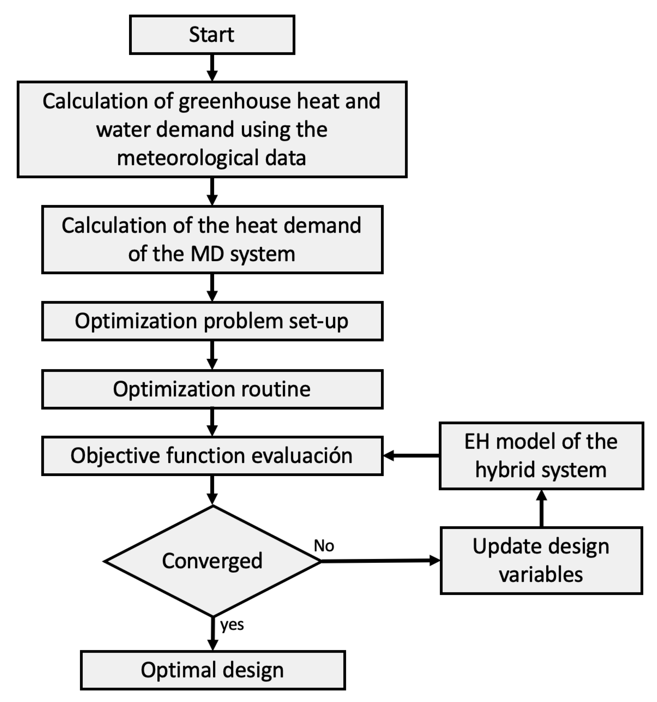
3. Design Optimization Method

The main objective of this work is to develop an operation-based optimization design method that exploits the synergies between the operational and design phases. In order to simultaneously take into account these phases, the developed algorithm was divided into two layers related to each other as shown in Figure 3. In the operational layer, a one-year meteorological dataset of the selected location is used to simulate the performance of the different subsystems. First, the thermal ($Q_g$) and water demands ($M_{trp}$) of the greenhouse are computed by means of its climate and humidity models, and then an EH model of the desalination facility is used to predict its thermal demand ($Q_D$).

Once both demands are calculated, they are used in the EH model of the solar-biomass system, which is governed by a rule-based control system in charge of ensuring the required thermal power to cover the demands. As presented in Figure 3, the sizing layer includes an optimization algorithm responsible for providing the optimal design of the system, according to a given objective function that attempts to ensure a sustainable energy supply by minimizing the biomass boiler contribution.

The communication between layers can be summarized as follows: (i) the sizing parameters provided by the optimization algorithm are sent to the operational layer to configure the EH model of the solar energy–biomass system, and (ii) in the operational layer, the one-year simulation is performed and the states of the different devices throughout it are sent to the sizing layer in order to calculate the new value of the objective function. This procedure is repeated until the optimization algorithm converges to the global solution. Figure 4 shows a detailed solving flowchart of the design algorithm to better clarify the aforementioned procedure. In addition, the following subsections depict each of the blocks presented in Figure 3.

3.1. Operational Layer: Thermal Demand Calculation

As mentioned above, the first step to carry out the optimal design of the hybrid system consists of predicting the thermal demand of both the greenhouse and the thermal desalination facility. The heat required by the greenhouse can be estimated using the climate model of this environment, as presented in [38]; hence, the temperature inside the greenhouse ($T_a$) can be calculated as follows:

$$c_a{\rho }_a\frac{{\mathrm{v}}_g}{{\mathrm{A}}_{ss}}\frac{d{T}_a}{dt}={\dot{q}}_{sol,a}+{\dot{q}}_{cv,ss-a}+{\dot{q}}_{heat}-{\dot{q}}_{cv,cnd-e}-{\dot{q}}_{ven}-{\dot{q}}_{trp},$$

(12)

where ${\dot{q}}_{sol,a}$ represents the radiative flux heating in the inside air through the cover, ${\dot{q}}_{cv,ss-a}$ is the convective flux with the soil surface, ${\dot{q}}_{heat}$ is the contribution of the heating system, ${\dot{q}}_{cv,cnd-e}$ is the convective heat transfer with the outside air, ${\dot{q}}_{ven}$ is the heat lost by natural ventilation and infiltration, and ${\dot{q}}_{trp}$ is the latent heat effect of crop transpiration. The remaining variables are presented in the Nomenclature section (see the Appendix A).

In addition, to calculate the thermal energy required by the thermal desalination plant, the water needs of the crops must be also estimated. This can be carried out by using the internal air humidity model of the greenhouse in which the humidity ($H_{abs,a}$) can be computed as [38]:

$${\rho }_a\frac{{\mathrm{v}}_a}{{\mathrm{A}}_{ss}}\frac{d{H}_{abs,a}}{dt}=M_{trp}-M_{vent},$$

(13)

where $M_{trp}$ is the crop transpiration flux, which represents the amount of water lost by the crops during the transpiration process and that must be supplied through irrigation, and $M_{vent}$ is the outflow by natural ventilation and infiltration. The remaining variables are also presented in the Nomenclature section.

The above equations were used in static mode for two reasons: on the one hand, to reduce the computational burden of the simulations as an entire year of meteorological data will be considered in the optimization routine, and, on the other, to directly link the climate model and the EH model within the optimization procedure. Thus, the temperature inside the greenhouse can be calculated at each sampling time as a function of the following meteorological variables:

$$T_a\left(k\right)=f(T_A\left(k\right),G\left(k\right),V_w\left(k\right)),$$

(14)

where $f(·)$ is a function of its arguments, and $V_w$ is the wind velocity. For this calculation, we assumed that the heating and ventilation systems of the greenhouse cannot be used at the same time. Thus, first, the temperature inside the greenhouse is calculated assuming that these two systems are turned off. Afterward, the heating or cooling needs are calculated based on the inner temperature set-point ($T_{SP}$), which means that, if the temperature inside the greenhouse is over $T_{SP}$, the ventilation must be used and the thermal contribution of this system is considered,

$${\dot{q}}_{ven}\left(k\right)=f(T_{SP}\left(k\right),T_A\left(k\right),G\left(k\right),V_w\left(k\right)),$$

(15)

otherwise, the heating system must be utilized to reach the set-point temperature and the heat flux needs to be taken into account instead,

$${\dot{q}}_{heat}\left(k\right)=f(T_{SP}\left(k\right),T_A\left(k\right),G\left(k\right),V_w\left(k\right)).$$

(16)

In this way, the heat flow rate needed by the greenhouse is given by Equation (17)

$${\dot{Q}}_g\left(k\right)=A_{ss}·{\dot{q}}_{heat}\left(k\right).$$

(17)

To calculate the needs of the thermal desalination facility, the crop transpiration flux is computed by using Equation (13) in static mode as a function of the following variables:

$$M_{trp}\left(k\right)=f(T_a\left(k\right),G\left(k\right),V_w\left(k\right),H_r\left(k\right)),$$

(18)

where $H_r$ is the external relative humidity. Then, the thermal needs of the desalination plant can be calculated using the EH methodology according to the Specific Thermal Energy Consumption (STEC) of the MD module as follows [39]:

$$\frac{{\dot{Q}}_D\left(k\right)}{M_{trp}\left(k\right)}=\frac{\delta ·A_{ss}·{\eta }_{ss}·STEC}{{\rho }_{wa}},$$

(19)

where ${\eta }_{ss}$ is related to the water losses in the substrate, $\delta$ is a conversion factor, and ${\rho }_{wa}$ is the water density.

3.2. Operational Layer: Rule-Based Control System of the Hybrid System

This system is used to deploy an operational scheme that guarantees the energy required by the greenhouse and the desalination system despite solar irradiance disturbances and demand variations. To this end, solar energy is considered as the primary energy source while the biomass boiler is used as backup. According to the above issues, the rule-based control algorithm can be summarized as follows:

• If the solar irradiance is higher than a threshold value, the solar field is turned on and the energy provided by this system is used to cover the demand.
• If the energy provided is higher than the demand, the surplus is stored in the storage system.
• Otherwise, either the remaining energy in the thermal storage tank (if any) is used to cover the demand or, if not, the biomass boiler is used instead.

3.3. Sizing Layer: Optimization Problem Statement

In line with the ideas presented in [26] for these kinds of systems, the objective function of the sizing optimization algorithm is aimed at minimizing the BPUI. In other words, the optimal solution consists of minimizing the contribution of the biomass boiler to ensure a sustainable energy supply. However, this optimization problem must be constrained to avoid an oversized solar field and storage system. Therefore, the energy balance over the entire simulation period in the operational layer, concerning the contribution of the heating system (both $Q_{sf}$ and $Q_{BB}$), the demands ($Q_D$ and $Q_g$), and the thermal losses in the storage device ($Q_{loss}$, this term is computed based on the storage degradation in Equation (5)) needs to be added as a constraint to ensure economic profitability of the designed system, and the optimization problem can be formulated as follows:

$$\begin{array}{cc}\hfill & \underset{{\dot{Q}}_{BB}^{max},A_{sf},Q_s^{max}}{min}BPUI,\hfill \\ \hfill \mathrm{subject}\mathrm{to}:& \sum _{k=1}^p{Q}_{sf}\left(k\right)+Q_{BB}\left(k\right)-Q_g\left(k\right)-Q_D\left(k\right)-Q_{loss}\left(k\right)=0,\hfill \\ \hfill & L_{BB}\le {\dot{Q}}_{BB}^{max}\le U_{BB},\hfill \\ \hfill & L_{sf}\le A_{sf}\le U_{sf},\hfill \\ \hfill & L_s\le Q_s^{max}\le U_s,\hfill \end{array}$$

(20)

where L and U are related to the lower and upper bounds of the design parameter of the respective systems. To solve the optimization problem, a genetic algorithm [40] ensures convergence toward a global solution given the nonlinear behaviour of the objective function. Furthermore, to avoid the complete evaluation of infeasible solutions in the operational layer (which, for a one-year period, is quite time consuming), if, at any sampling time, the energy demand cannot be covered by the power systems and the remaining energy in the storage tank, the simulation is aborted, and a high value, i.e., 10${}^6$, is considered as the cost of the objective function.

4. Results and Discussion

The case study based on the facilities described in Section 2 serves to illustrate the developed methodology in the design of a solar energy–biomass heating system for an isolated greenhouse environment, which has been adapted to replicate a real-world example of a small plot greenhouse holder. In this way, regarding the greenhouse included in the case study, the same greenhouse structure as the one described in Section 2 was used to configure the model. However, since this is a pilot-scale greenhouse, the results in terms of heat flux and crop transpiration were extrapolated to a crop cultivation area of 1 ha, which is more representative of small–medium farms in the province of Almería [41].

The set-point temperature to calculate the heating demand was established at 14 and 21 °C for the night and day periods, respectively, whereas the relative humidity inside the greenhouse was constrained between 40–90%. Both the temperature and humidity operating conditions were chosen following the recommendations provided in [42] for tomato cultivation, the type of crop considered in this study. To provide a more realistic case, we assumed that two cultivation campaigns were carried out over the simulated year, one long campaign, from September to May, and a short one, from June to July, while August was devoted to carry out maintenance work, with no crops inside the greenhouse. This reproduces the timing and operating conditions that are usually used in the province of Almería for tomatoes.

With regard to the EH model of the solar energy–biomass system and the desalination plant, the setting parameters used to configure it are shown in

Table 1. Value of the parameters of the EH model.

	ηb1 [-]	HV 2 [kWh/kg]	ηo3 [-]	α3 [W/(m2K)]	β3 [W/(m2K3)]	ηs4 [-]	ηch4 [-]	ηdis4 [-]	ηss5 [-]	STEC 6 [kWh/m3]
Value	0.8	4.86	0.775	3.723	0.016	0.95	0.98	0.98	1.2	106.6

^1. Obtained from [34]. ^2. Obtained from the database of the European Biomass Industry Association [43], considering, as biomass, Pellets at 8% moist. ^3. Obtained from collector’s certification [44]. ^4. Obtained from [45]. ^5. Obtained from the operation experience in the real greenhouse. ^6. Obtained from [46] considering the optimal operating conditions reported in that study.

, as well as the sources from which their values were obtained. Most of the parameters come from certification or experimental tests performed in the actual facilities. In addition, the threshold irradiance value used in the rule-based controller to turn on the solar field was fixed at 250 W/m${}^2$ following the typical strategies used in solar thermal fields [28].

For the simulation and design of systems, Meteornorm v7 Typical Meteorological Year (TMY) for a representative coastal location at the province of Almería was used to conduct corresponding model calculations on an hourly basis [47]. TMY data were checked for consistency with the daily records of an available twenty year agro-climatic station in close vicinity of the selected greenhouse placement [48]. The overall meteorological conditions that mostly affect the greenhouse indoor climate, i.e., the irradiation and ambient temperature, are presented in Figure 5 on a monthly basis. Note that the total global irradiation along the year was 1827 kWh/m${}^2$.

The algorithm was programmed in MATLAB code (release 2020b), and the genetic algorithm used to solve the optimization problem is included in the Global Optimization Toolbox of this software (the reader can find further information about it in [49]). The code was run on a PC with an Intel Core i7 CPU 2.5 GHz (four cores) and 16 GB of RAM.

The remaining subsections show and discuss the optimization and analysis of the hybrid solar energy–biomass heating network. First, the results of the optimization procedure that identifies the optimal sizing of the system are presented. Second, the optimized plant performance is depicted by showing several weeks of system operation for the year under consideration. Lastly, the solution provided by the algorithm is analysed taking into account different aspects and putting special attention toward the economic viability of the hybrid using LCOH and the discount payback period.

4.1. Optimal Design

As commented, the ga algorithm from MATLAB was used to solve the optimization problem. This algorithm allowed us to deal with the nonlinear behaviour of both the objective function and the constraint related to the energy balance of the system, as presented in the formulation of the optimization problem in Equation (20). Within the optimization procedure, a complete year of meteorological data on an hourly basis was considered. The main advantage of taking into account data on such a small time scale is that it allowed us to make a much more accurate design of the hybrid heating system, considering the time-varying demands of the greenhouse and desalination facility (see Figure 6).

However, this detailed simulation significantly penalized the solving time of the optimization problem. For this reason, the $ga$ algorithm was configured to be executed in parallel, trying to take advantage of all the hardware resources available in the PC, i.e., the four cores, to reduce the solving time. The bounds in

Table 2. The upper and lower bounds used in the optimization problem.

	Lower Bound, ${\mathit{L}}_{\mathit{i}}$	Upper Bound, ${\mathit{U}}_{\mathit{i}}$
$A_{ss}$	0	10,000
${\dot{Q}}_{BB}^{max}$	0	6000
$Q_s^{max}$	0	10,000

were used in the optimization problem to limit the search space. In this way, the time required to solve the problem was around 20 min, leading to the results summarized in

Table 3. Values of the optimal sizing parameters and performance metrics.

	Optimal Sizing Parameters			Performance Metrics
	${\mathit{A}}_{\mathit{s}\mathit{f}}$	${\dot{\mathit{Q}}}_{\mathit{B}\mathit{B}}^{\mathit{m}\mathit{a}\mathit{x}}$	${\mathit{Q}}_{\mathit{s}}^{\mathit{m}\mathit{a}\mathit{x}}$	SF	BF	BPUI
	[m${}^{\mathbf{2}}$]	[kW]	[kWh]	[-]	[-]	[-]
Value	266	4234	425	0.16	0.84	5.25

.

The optimal size of the solar field was found to be around 266 m${}^2$, the thermal storage system has a maximum capacity of 425 kWh, whereas the optimal maximum capacity of the biomass system takes a value of 4234 kW (note that this value refers to the total biomass-generated power, not a single boiler). This configuration led to a solar fraction of 16%, and, consequently, to a biomass fraction of 84%. The relatively low solar fraction was due to the heterogeneous demand of the system. Although the accumulated demand of both systems was balanced, the greenhouse represented the 51% of the total demand and the desalination facility represented the remaining 49%, the greenhouse’s demand appeared mainly in the form of sharp peaks during the night periods in the winter months (see Figure 6). This prevented an increase in the solar fraction since it would give rise to oversized designs of the solar field and thermal storage tank that would not be justified taking into account the demand during the rest of the year, which was more homogeneous since it was attributed only to the desalination plant (see Figure 6). In June, the demand of the desalination plant was lower since it coincided with the start of the second growing season (the demand for water, and therefore for heat, increases as the plants grow), while, in August, there was no demand as there were no crops inside the greenhouse as commented above.

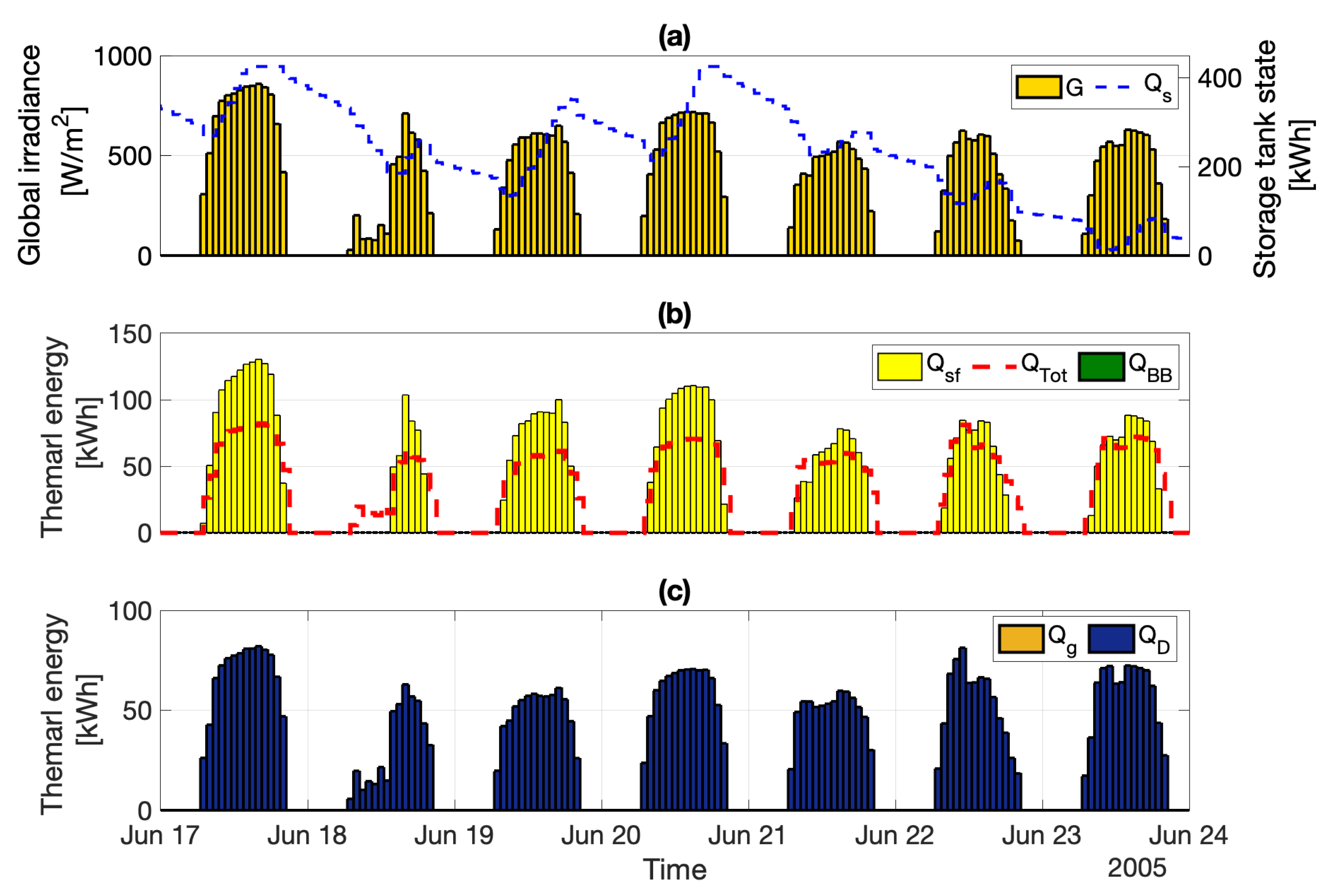
4.2. Optimized Plant Performance

This section shows two weeks of operation at two different periods of the year to demonstrate the performance of the optimized hybrid system in the daily operation. The first one corresponds to the week of 7 to 14 January and is presented in Figure 7. In this case, there was thermal demand both from the greenhouse, for heating, as it was a cold month, and from the desalination plant, to cover the irrigation water needs (see Figure 7c). The main peculiarity that occurs in this case is that the two demands are decoupled in time, that is, the heating demand of the greenhouse is predominant at night, while the demand of the desalination plant is higher during the day since the transpiration of the crops is directly related to the solar irradiance. This disparity supports the application of the proposed design optimization method using an hourly basis simulation to undertake an adequate demand-side design.

The scheduling performed by the rule-based control can be seen in Figure 7b. On the first, second, and third days, as the global irradiance was over the threshold value, the thermal demand of the desalination plant was covered using the entire energy provided by the solar field and using the biomass boiler as backup. During the night, as there was no room to store energy in the thermal storage tank due to the irradiance conditions and high demand during the day (see Figure 7a), the heating demand of the greenhouse was totally covered with the biomass boiler. Something similar happened in the rest of the days in which, due to the low availability of irradiance typical at this time of the year (more likely to have partially or totally overcast skies), the solar field could hardly be operated, and almost all the energy was covered with the biomass boiler.

The second week corresponded to the week of 17–24 June and is displayed in Figure 8. Here, the panorama was different from the one shown previously. First, there was no demand for heating as it was a summer month, and, secondly, the thermal demand from the desalination plant was lower than in the previous case (see Figure 8c). The latter occurred since the size of the crops was smaller as it was almost at the beginning of the second growing season. In this way, it can be observed how the rule-based control system used part of the energy provided by the solar field to meet the demand of the desalination plant (see Figure 8b), while the rest was stored in the tank (see Figure 8a).

This allowed, on days with lower irradiance values or with disturbances, such as the second day of the week shown, part of the energy stored in the tank could be used to cover the demand, avoiding the operation of the biomass boiler (see Figure 8b) and, thus, leading to a much more sustainable and efficient operation of the hybrid system in terms of emissions.

4.3. Analysis of the Optimal Solution

The solution provided by the algorithm must be evaluated in terms of not only the technical feasibility but also the economic, social, and environmental impacts in order to address sustainability. As the plant’s layout is already bound, up to a certain point, to the two latter issues in the Almerian agricultural system (all the energy carriers are renewable, part of the biomass can come from agricultural waste, and desalination contributes to reducing the overexploitation of aquifers), no externalities, such as ecosystem impacts and/or resource limits, were considered. Only the economic viability was studied to evidence the effectiveness of the proposed design method. For this purpose, the LCOH and discount payback period of the given solution were analysed using the nominal values presented in

Table 4. The purchase prices considered for each device, the investment costs of the solution delivered by the algorithm, the operating and maintenance costs, the discount rate, and the life time of the plant. The values reported in the last three rows are used for the three devices, i.e., the solar field, biomass boiler, and thermal storage tank.

	Cost/Unit	${\mathit{C}}_{\mathit{I}\mathit{n}\mathit{v}}$ [€]	${\mathit{C}}_{\mathit{O}}$	${\mathit{C}}_{\mathit{M}}$	r	N [Years]
Solar field	200 ${}^a$ €/m${}^2$	53,200	0.009 ${}^d$ kW/m${}^2$	0.5% e of $C_{Inv}$	3% ${}^f$	25
Biomass boiler	Power law rule ${}^b$	491,860	0.225 ${}^d$ €/kg
Thermal storage tank	62 ${}^c$ €/kW	26,350	-

^a Obtained from the work in [50], ^b calculated through the power law rule according to the ideas presented in [51], ^c obtained from the work in [26], ^d obtained from reference [52] (considering also the same electricity price of that work to calculate the operating cost of the solar field), ^e obtained from reference [53], ^f obtained from [54].

to configure the economic model.

The first economic metric evaluated was the LCOH, which gives information about the cost of the energy produced by each device. The value of the LCOH for the solar thermal field was found to be around 0.035 €/kWh, and the biomass boiler was 0.078 €/kWh. These figures are in agreement with the LCOH values reported in the literature for similar applications. For example, in the case of the solar thermal field, an LCOH of around 0.03 €/kWh was obtained in [53], whereas, in the case of the biomass boiler, LCOH values ranging from 0.07 to 0.10 €/kWh, depending on the biomass price, were disclosed in [26].

This demonstrates the adequacy of the solution provided by the algorithm. The LCOH values can also be compared to other energy sources employed in these kinds of environments, especially fossil fuels, which tend to be the economical alternative at the expense of their environmental impact. As discussed in [31], gas and diesel boilers are normally used for providing heat to greenhouses, especially in isolated areas. The base price of natural gas is 0.05 €/kWh, which may be higher if there is no nearby natural gas distribution network, whereas diesel fuel can reach 0.45 €/kWh in off-grid locations [55].

These reference prices prove the viability of the designed hybrid system, even without considering the environmental benefits, and suggest that it is especially attractive to be implemented in rural areas without access to the natural gas distribution network, in which the price of this resource could be higher than the reference value because of the transportation costs, or, directly, diesel could be the only option available.

The second economic indicator analysed was the discount payback period. This metric is highly dependent on the fuel price considered for comparison purposes, as this price influences the term $C_{savings}$ in Equation (11). For this reason, several fuel prices from 0.01 to 0.45 €/kWh were taken into account to perform a sensitivity analysis as shown in Figure 9. This range was chosen to encompass the price that a conventional source, such as natural gas can reach in different countries considering the supply and demand particular conditions, the national energy mix, geopolitical situation, network costs, import diversification, environmental protection costs, or levels of excise and taxation [56], and, also, the price that this kind of conventional sources can attain in isolated rural environments, i.e., 0.45 €/kWh [55].

In this way, as observed in Figure 9, for the case of a fuel price of 0.05 €/kWh (nominal price of the natural gas) the discount payback period was 13 years. Although this is a relatively high value, it is within the useful life of the system confirming its economic profitability. Nevertheless, this result improved considerably as the price of fuel increased, reaching periods of 4 years when compared to a fuel price of 0.08 €/kWh and of around one year from a price of 0.25 €/kWh onwards. This means that, in locations where diesel is the only option, the use of the hybrid system is much more profitable, and the investment cost of the hybrid facility can be recovered almost immediately. Finally, it should also be noted that, for prices below 0.05 €/kWh, the investment is not profitable.

5. Conclusions

This paper demonstrates that sustainable farming solutions, within the WEF nexus approach, can be carried out by implementing EH-based models and renewable hybrid systems for energy production. In particular, a demand-side optimization algorithm for sizing solar energy–biomass plants was proposed to be implemented in isolated greenhouse environments. An opportunity for agriculture presents itself as this innovative method of designing systems may ease decision-making for farmers, on whom the burden of the transition to sustainable farming systems might be unduly placed in the near future. The main findings that can be drawn from this study are:

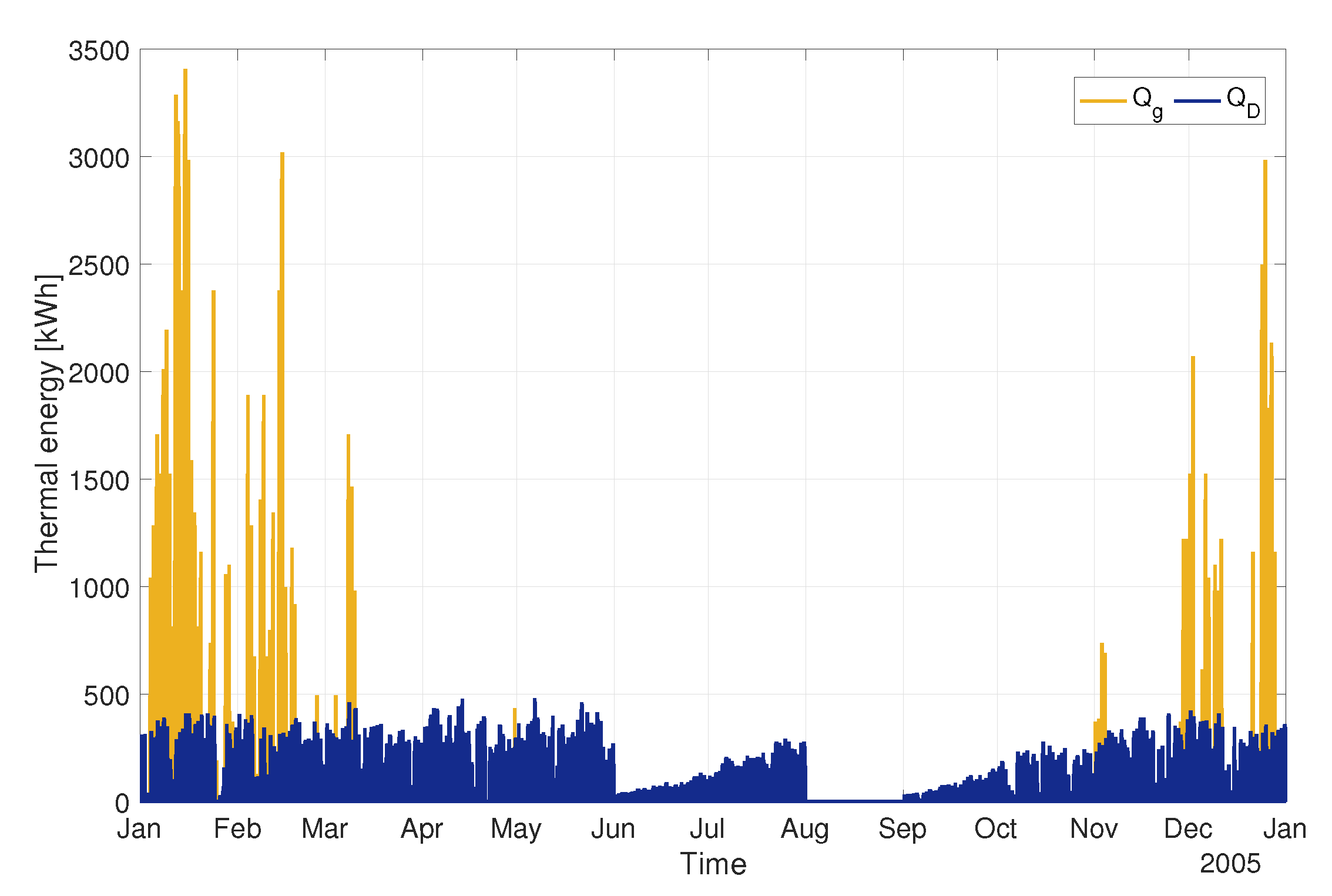
• The proposed algorithm resulted in a powerful tool to carry out demand-side design of solar-biomass hybrid systems for greenhouse environments. Its use is especially recommended for applications where the demand is heterogeneous, such as for the case study conducted. There was a high demand for heating during the winter months and a more homogeneous demand during the rest of the year due to the thermal consumption of the desalination plant used to provide the irrigation water.
• The use of the EH modelling methodology was proven to be an effective mechanism for bridging the design and operation phases. This methodology allowed us to evaluate, in a simple and fast way, each of the designs proposed by the optimization algorithm during a full year of operation. This resulted in a much more adequate design of the system and avoided the oversizing of key elements for the economic profitability of the system, such as the solar field and the thermal storage tank.
• Regarding the case study, the results revealed an optimal solar fraction for the considered location (Almería province) and greenhouse size (1 ha) of 16%. With this solar fraction, the system was able to cover almost the complete thermal demand of the desalination facility during hot months where there was no heat demand from the greenhouse.
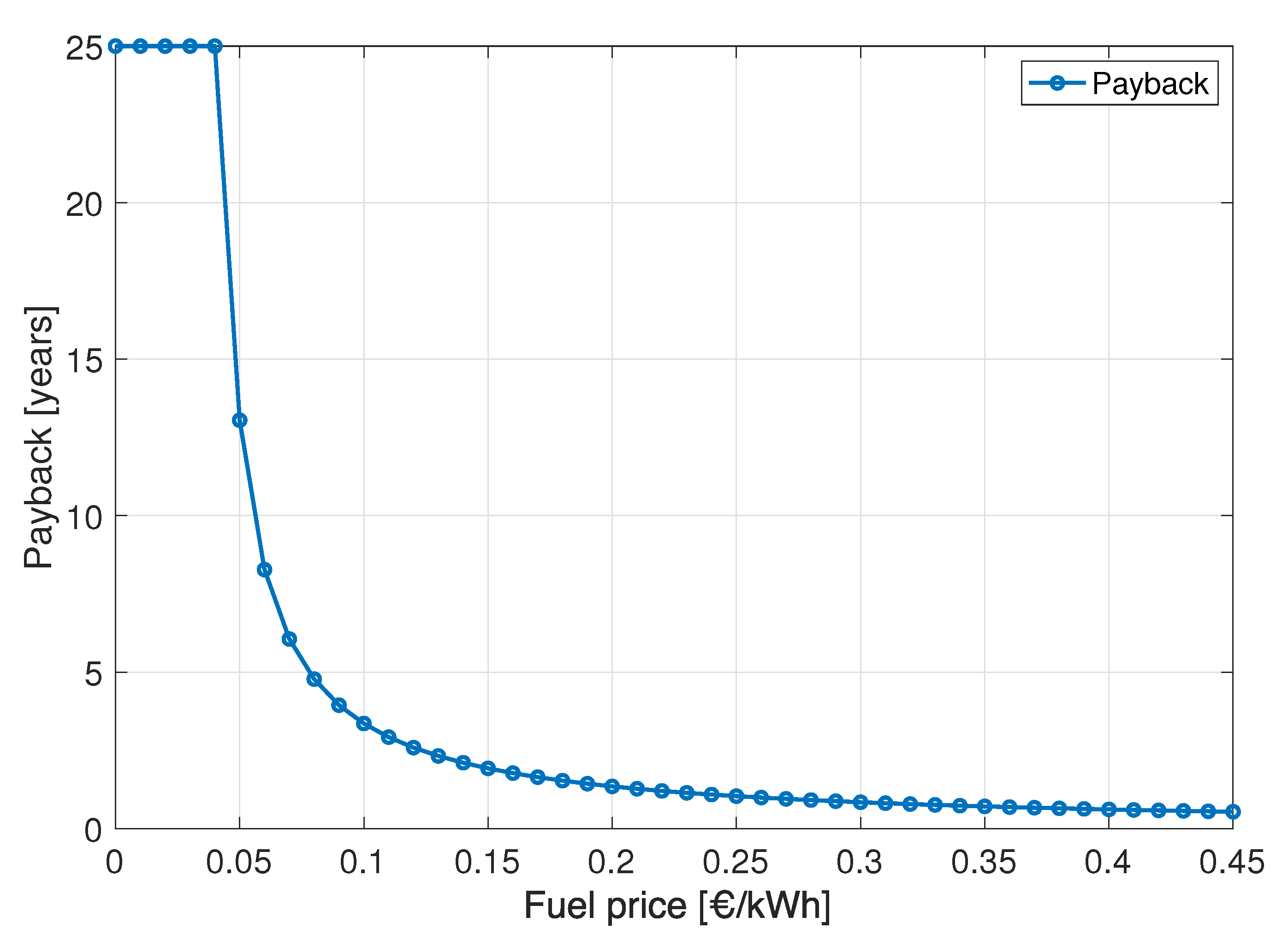
• Finally, the economic evaluation performed in terms of the LCOH and discount payback period confirmed the adequacy and viability of the solution provided by the design algorithm, especially for isolated areas where the price of conventional sources can be relatively high due to transportation issues.

Future work will focus on extending the design technique to multi-objective optimization frameworks that consider economic, technical, and environmental issues, which normally conflict in these kinds of systems. Moreover, further studies on the control system of the operational layer will be performed. In this article, a rule-based controller was employed that was proven to be effective for design purposes; however, for practical situations where irradiance disturbances play a major role, the use of advanced control techniques, such as model predictive controllers, is more appropriate and could become essential for the successful implementation of solar-energy biomass systems in real-world applications.

References

1. Irabien, A.; Darton, R. Energy–water–food nexus in the Spanish greenhouse tomato production. Clean Technol. Environ. Policy 2016, 18, 1307–1316. [Google Scholar] [CrossRef]
2. Martinez, P.; Blanco, M.; Castro-Campos, B. The water–energy–food nexus: A fuzzy-cognitive mapping approach to support nexus-compliant policies in Andalusia (Spain). Water 2018, 10, 664. [Google Scholar] [CrossRef] [Green Version]
3. Aquastat, F. Information System on Water and Agriculture. Available online: http://www.fao.org/aquastat/en/overview/methodology/water-use (accessed on 9 June 2021).
4. Velasco-Muñoz, J.F.; Aznar-Sánchez, J.A.; Belmonte-Ureña, L.J.; Román-Sánchez, I.M. Sustainable water use in agriculture: A review of worldwide research. Sustainability 2018, 10, 1084. [Google Scholar] [CrossRef] [Green Version]
5. Hipólito-Valencia, B.J.; Mosqueda-Jiménez, F.W.; Barajas-Fernández, J.; Ponce-Ortega, J.M. Incorporating a seawater desalination scheme in the optimal water use in agricultural activities. Agric. Water Manag. 2021, 244, 106552. [Google Scholar] [CrossRef]
6. Mehmood, A.; Ren, J. Renewable energy-driven desalination for more water and less carbon. In Renewable-Energy-Driven Future; Elsevier: Amsterdam, The Netherlands, 2021; pp. 333–372. [Google Scholar]
7. Aznar-Sánchez, J.A.; Belmonte-Ureña, L.J.; Velasco-Muñoz, J.F.; Valera, D.L. Farmers’ profiles and behaviours toward desalinated seawater for irrigation: Insights from South-east Spain. J. Clean. Prod. 2021, 296, 126568. [Google Scholar] [CrossRef]
8. Quist-Jensen, C.A.; Macedonio, F.; Drioli, E. Membrane technology for water production in agriculture: Desalination and wastewater reuse. Desalination 2015, 364, 17–32. [Google Scholar] [CrossRef]
9. Gil, J.D.; Roca, L.; Berenguel, M. Modelling and automatic control in solar membrane distillation: Fundamentals and proposals for its technological development. Rev. Iberoam. Autom. Inform. Ind. 2020, 17, 329–343. [Google Scholar] [CrossRef]
10. Gil, J.D.; Álvarez, J.D.; Roca, L.; Sánchez-Molina, J.; Berenguel, M.; Rodríguez, F. Optimal thermal energy management of a distributed energy system comprising a solar membrane distillation plant and a greenhouse. Energy Convers. Manag. 2019, 198, 111791. [Google Scholar] [CrossRef]
11. Bouchrit, R.; Boubakri, A.; Hafiane, A.; Bouguecha, S.A.T. Direct contact membrane distillation: Capability to treat hyper-saline solution. Desalination 2015, 376, 117–129. [Google Scholar] [CrossRef]
12. Deshmukh, A.; Boo, C.; Karanikola, V.; Lin, S.; Straub, A.P.; Tong, T.; Warsinger, D.M.; Elimelech, M. Membrane distillation at the water-energy nexus: Limits, opportunities, and challenges. Energy Environ. Sci. 2018, 11, 1177–1196. [Google Scholar] [CrossRef]
13. Aschilean, I.; Rasoi, G.; Raboaca, M.S.; Filote, C.; Culcer, M. Design and concept of an energy system based on renewable sources for greenhouse sustainable agriculture. Energies 2018, 11, 1201. [Google Scholar] [CrossRef] [Green Version]
14. Esen, M.; Yuksel, T. Experimental evaluation of using various renewable energy sources for heating a greenhouse. Energy Build. 2013, 65, 340–351. [Google Scholar] [CrossRef]
15. Taki, M.; Rohani, A.; Rahmati-Joneidabad, M. Solar thermal simulation and applications in greenhouse. Inf. Process. Agric. 2018, 5, 83–113. [Google Scholar] [CrossRef]
16. Shekarchi, N.; Shahnia, F. A comprehensive review of solar-driven desalination technologies for off-grid greenhouses. Int. J. Energy Res. 2019, 43, 1357–1386. [Google Scholar] [CrossRef]
17. Attar, I.; Naili, N.; Khalifa, N.; Hazami, M.; Farhat, A. Parametric and numerical study of a solar system for heating a greenhouse equipped with a buried exchanger. Energy Convers. Manag. 2013, 70, 163–173. [Google Scholar] [CrossRef]
18. Lazaar, M.; Bouadila, S.; Kooli, S.; Farhat, A. Comparative study of conventional and solar heating systems under tunnel Tunisian greenhouses: Thermal performance and economic analysis. Sol. Energy 2015, 120, 620–635. [Google Scholar] [CrossRef]
19. Attar, I.; Farhat, A. Efficiency evaluation of a solar water heating system applied to the greenhouse climate. Sol. Energy 2015, 119, 212–224. [Google Scholar] [CrossRef]
20. Zhang, C.; Sun, J.; Lubell, M.; Qiu, L.; Kang, K. Design and simulation of a novel hybrid solar-biomass energy supply system in northwest China. J. Clean. Prod. 2019, 233, 1221–1239. [Google Scholar] [CrossRef]
21. Bilandzija, N.; Voca, N.; Jelcic, B.; Jurisic, V.; Matin, A.; Grubor, M.; Kricka, T. Evaluation of Croatian agricultural solid biomass energy potential. Renew. Sustain. Energy Rev. 2018, 93, 225–230. [Google Scholar] [CrossRef]
22. Morone, P.; Falcone, P.M.; Tartiu, V.E. Food waste valorisation: Assessing the effectiveness of collaborative research networks through the lenses of a COST action. J. Clean. Prod. 2019, 238, 117868. [Google Scholar] [CrossRef]
23. Garcia-Herrero, I.; Hoehn, D.; Margallo, M.; Laso, J.; Bala, A.; Batlle-Bayer, L.; Fullana, P.; Vazquez-Rowe, I.; Gonzalez, M.; Durá, M.; et al. On the estimation of potential food waste reduction to support sustainable production and consumption policies. Food Policy 2018, 80, 24–38. [Google Scholar] [CrossRef]
24. Ng, W.J.; Xiao, K.; Tyagi, V.K.; Pan, C.; Poh, L.S. Food Waste and Biomass Recovery. In Oxford Research Encyclopedia of Environmental Science; Oxford University Press: Oxford, UK, 2019. [Google Scholar]
25. Despoudi, S.; Bucatariu, C.; Otles, S.; Kartal, C. Food waste management, valorization, and sustainability in the food industry. In Food Waste Recovery; Academic Press: Cambridge, MA, USA, 2021; pp. 3–19. [Google Scholar]
26. Tilahun, F.B.; Bhandari, R.; Mamo, M. Design optimization of a hybrid solar-biomass plant to sustainably supply energy to industry: Methodology and case study. Energy 2021, 220, 119736. [Google Scholar] [CrossRef]
27. Geidl, M.; Koeppel, G.; Favre-Perrod, P.; Klöckl, B.; Andersson, G.; Fröhlich, K. Energy hubs for the future. IEEE Power Energy Mag. 2006, 5, 24–30. [Google Scholar] [CrossRef]
28. Gil, J.D.; Roca, L.; Zaragoza, G.; Normey-Rico, J.E.; Berenguel, M. Hierarchical control for the start-up procedure of solar thermal fields with direct storage. Control Eng. Pract. 2020, 95, 104254. [Google Scholar] [CrossRef] [Green Version]
29. Sánchez-Molina, J.; Reinoso, J.; Acién, F.; Rodríguez, F.; López, J. Development of a biomass-based system for nocturnal temperature and diurnal CO2 concentration control in greenhouses. Biomass Bioenergy 2014, 67, 60–71. [Google Scholar] [CrossRef]
30. Herranz de Rafael, G.; Fernández-Prados, J.S. Intensive agriculture, marketing and social structure: The case of South-eastern Spain. Agric. Econ. 2018, 64, 367–377. [Google Scholar]
31. Valera, D.; Belmonte, L.; Molina, F.; López, A. Greenhouse Agriculture in Almería: A Comprehensive Techno-Economic Analysis; Cajamar: Almería, Spain, 2016. [Google Scholar]
32. Ruiz-Aguirre, A.; Andrés-Mañas, J.; Fernández-Sevilla, J.; Zaragoza, G. Comparative characterization of three commercial spiral-wound membrane distillation modules. Desalin. Water Treat. 2017, 61, 152–159. [Google Scholar]
33. Zaragoza, G.; Ruiz-Aguirre, A.; Guillén-Burrieza, E. Efficiency in the use of solar thermal energy of small membrane desalination systems for decentralized water production. Appl. Energy 2014, 130, 491–499. [Google Scholar] [CrossRef]
34. Vallios, I.; Tsoutsos, T.; Papadakis, G. Design of biomass district heating systems. Biomass Bioenergy 2009, 33, 659–678. [Google Scholar] [CrossRef]
35. Allouhi, A.; Agrouaz, Y.; Amine, M.B.; Rehman, S.; Buker, M.; Kousksou, T.; Jamil, A.; Benbassou, A. Design optimization of a multi-temperature solar thermal heating system for an industrial process. Appl. Energy 2017, 206, 382–392. [Google Scholar] [CrossRef]
36. Duffie, J.A.; Beckman, W.A. Solar Engineering of Thermal Processes; John Wiley & Sons, Inc.: Hoboken, NJ, USA, 2013. [Google Scholar] [CrossRef]
37. Ali, B. Techno-economic optimization for the design of solar chimney power plants. Energy Convers. Manag. 2017, 138, 461–473. [Google Scholar] [CrossRef]
38. Rodríguez, F.; Berenguel, M.; Guzmán, J.L.; Ramírez-Arias, A. Modeling and Control of Greenhouse Crop Growth; Springer: Berlin/Heidelberg, Germany, 2015. [Google Scholar]
39. Gil, J.D.; Ruiz-Aguirre, A.; Roca, L.; Zaragoza, G.; Berenguel, M. Prediction models to analyse the performance of a commercial-scale membrane distillation unit for desalting brines from RO plants. Desalination 2018, 445, 15–28. [Google Scholar] [CrossRef] [Green Version]
40. Golberg, D.E. Genetic Algorithms in Search, Optimization, and Machine Learning; Addion Wesley: Boston, MA, USA, 1989; Volume 1989, p. 36. [Google Scholar]
41. Galdeano-Gómez, E.; Aznar-Sánchez, J.A.; Pérez-Mesa, J.C. Sustainability dimensions related to agricultural-based development: The experience of 50 years of intensive farming in Almería (Spain). Int. J. Agric. Sustain. 2013, 11, 125–143. [Google Scholar] [CrossRef]
42. Shamshiri, R.R.; Jones, J.W.; Thorp, K.R.; Ahmad, D.; Che Man, H.; Taheri, S. Review of optimum temperature, humidity, and vapour pressure deficit for microclimate evaluation and control in greenhouse cultivation of tomato: A review. Int. Agrophys. 2018, 32, 287–302. [Google Scholar] [CrossRef]
43. EUBIA. European Biomass Industry Association. Biomass Characteristics. 2021. Available online: https://www.eubia.org/cms/wiki-biomass/biomass-characteristics-2/ (accessed on 28 April 2021).
44. BOE. Certification of Solar Collectors SOLARIS CP1—NOVA. 2014. Available online: https://www.boe.es/boe/dias/2014/07/02/pdfs/BOE-A-2014-6950.pdf (accessed on 28 April 2021).
45. Evins, R. Multi-level optimization of building design, energy system sizing and operation. Energy 2015, 90, 1775–1789. [Google Scholar] [CrossRef]
46. Ruiz-Aguirre, A.; Andrés-Mañas, J.; Fernández-Sevilla, J.; Zaragoza, G. Experimental characterization and optimization of multi-channel spiral wound air gap membrane distillation modules for seawater desalination. Sep. Purif. Technol. 2018, 205, 212–222. [Google Scholar] [CrossRef]
47. Remund, J.; Muller, S.; Kunz, S.; Huguenin-Landl, B.; Studer, C.; Cattin, R. Global Meteorological Database Version 7 Software and Data for Engineers, Planers and Education; Genossenschaft Meteotest: Bern, Switzerland, 2017; pp. 1–17. [Google Scholar]
48. RIA. Red de Información Agroclimática de Andalucía. 2021. Available online: https://www.juntadeandalucia.es/agriculturaypesca/ifapa/riaweb/web/inicio_estaciones (accessed on 28 April 2021).
49. MATLAB. MATLAB Optimization Toolbox Release 2020b; The MathWorks: Natick, MA, USA, 2020. [Google Scholar]
50. Meyers, S.; Schmitt, B.; Vajen, K. A Comparative Cost Assessment of Low Carbon Process Heat between Solar Thermal and Heat Pumps. In Proceedings of the ISES Solar World Congress 2017, Abu Dhabi, United Arab Emirates, 29 October–2 November 2017. [Google Scholar]
51. Chau, J.; Sowlati, T.; Sokhansanj, S.; Preto, F.; Melin, S.; Bi, X. Economic sensitivity of wood biomass utilization for greenhouse heating application. Appl. Energy 2009, 86, 616–621. [Google Scholar] [CrossRef]
52. Ramos-Teodoro, J.; Gil, J.D.; Roca, L.; Rodríguez, F.; Berenguel, M. Optimal Water Management in Agro-Industrial Districts: An Energy Hub’s Case Study in the Southeast of Spain. Processes 2021, 9, 333. [Google Scholar] [CrossRef]
53. Semple, L.; Carriveau, R.; Ting, D.S.K. A techno-economic analysis of seasonal thermal energy storage for greenhouse applications. Energy Build. 2017, 154, 175–187. [Google Scholar] [CrossRef]
54. Tian, Z.; Perers, B.; Furbo, S.; Fan, J. Thermo-economic optimization of a hybrid solar district heating plant with flat plate collectors and parabolic trough collectors in series. Energy Convers. Manag. 2018, 165, 92–101. [Google Scholar] [CrossRef] [Green Version]
55. Soltero, V.; Chacartegui, R.; Ortiz, C.; Velázquez, R. Potential of biomass district heating systems in rural areas. Energy 2018, 156, 132–143. [Google Scholar] [CrossRef]
56. Eurostat. Natural Gas Price Statistics. 2020. Available online: https://ec.europa.eu/eurostat/statistics-explained/index.php?title=Natural_gas_price_statistics (accessed on 9 June 2021).
Figure 1. Supply and demand agents in the greenhouse environment.
Energies 14 03724 g001
Figure 2. The Energy Hubs (EH) schematic diagram from which the mathematical model is derived.
Energies 14 03724 g002
Figure 3. Schematic diagram of the design optimization algorithm.
Energies 14 03724 g003
Figure 4. The solving flowchart diagram.
Energies 14 03724 g004
Figure 5. The monthly global irradiation and mean temperature of the Typical Meteorological Year (TMY) used.
Energies 14 03724 g005
Figure 6. Distribution of the hourly thermal demand of the greenhouse ( Q g ) and desalination facility ( Q D ) throughout the year under consideration.
Energies 14 03724 g006
Figure 7. Simulation results during the week of 7 to 14 January. (a) Global irradiance (G) and storage tank state ( Q s ), (b) the total thermal energy demand of the system ( Q T o t ), contribution of the biomass boiler ( Q B B ) and contribution of the solar field ( Q s f ), and (c) the greenhouse thermal energy demand ( Q g ) and thermal desalination facility demand ( Q D ).
Energies 14 03724 g007
Figure 8. Simulation results during the week of 17 to 24 June. (a) Global irradiance (G) and storage tank state ( Q s ), (b) the total thermal energy demand of the system ( Q T o t ), contribution of the biomass boiler ( Q B B ) and contribution of the solar field ( Q s f ), and (c) the greenhouse thermal energy demand ( Q g ) and thermal desalination facility demand ( Q D ).
Energies 14 03724 g008
Figure 9. The discount payback period as a function of different fuel prices.
Energies 14 03724 g009