Article

Reliability and Economic Evaluation of Offshore Wind Power DC Collection Systems

1
School of Electrical Engineering, Zhengzhou University, Zhengzhou 450001, China
2
School of Engineering, Cardiff University, Cardiff CF24 3AA, UK
*
Author to whom correspondence should be addressed.
Energies 2021, 14(10), 2922; https://doi.org/10.3390/en14102922
Submission received: 16 April 2021 / Revised: 12 May 2021 / Accepted: 14 May 2021 / Published: 18 May 2021
(This article belongs to the Special Issue Innovative HVDC and MVDC Connection Schemes for Offshore Wind Farms)

Abstract

:
One key directive to realize the global transition towards net-zero emission goals is to integrate more renewable energy resources into the generation mix. Due to higher and more consistent wind speeds, offshore wind farms (OWFs) have the potential to generate more energy at a steadier rate than their onshore counterpart. However, at the collection system level, all the OWFs use alternating current (AC) technology at present. Nonetheless, with an increasing capacity of the single wind turbine (WT) and larger distances to the shore, the use of direct current (DC) technology at the collection system level is beneficial. To select a suitable DC collection system topology, this paper proposes a comprehensive analytical reliability evaluation method, based on the Universal Generating Function technique, together with associated economic factors. Four candidates DC collection system options were evaluated with different WT capacities for a 400 MW OWF. The availability indices such as Generation Ratio Availability and Expected Energy Not Supplied were used to assess their reliability levels. The results show that the radial topology with a single platform DC/DC converter is more reliable and economical than the other candidate options.

1. Introduction

1.1. Background

Power generation that utilizes naturally replenishing resources shows significant advantages over coal- and fossil fuel-based power plants. Greenhouse gas emissions, depletion of resources over time, and emission of harmful substances are some of the major drawbacks of these thermal power plants. To minimize these impacts, various policy goals have been set by different nations across the globe. The UK’s ambition to be net-zero by 2050 [1] and the European Union’s target to become carbon neutral by 2050 [2] are some of the strategic decisions already established. Further, China also devised aspiring targets to become carbon neutral before 2060 and plans to reduce its emissions within the next ten years [3]. All these goals will catalyze renewable energy (RE) development further.
Among the different state-of-the-art RE technologies, energy generation via wind resource accounts for a significant portion of the global RE mix. For instance, the energy generated by wind in 2019 was 1417.05 TWh [4]. Compared to onshore wind power, offshore wind power has advantages, such as richer wind resources, no land restrictions, and a higher capacity factor. Therefore, it has shown broader sustainable development prospects [5]. In 2019, the newly installed capacity of global offshore wind power exceeded 6 GW, with a cumulative installed capacity of 29.1 GW [6]. Notably, in the same year, China achieved a new record, installing 2.4 GW offshore wind [7].
With the significant advancements in offshore wind turbine (WT) technology, the rated capacity of a single unit has been increased over the last few years. In early 2021, Vestas announced a 15 MW wind turbine—V236-15.0 MW [8]. It is currently the largest WT in the world, with a prototype installation expected in 2022, and serial production scheduled for 2024. Further, the GE 14 MW Haliade-X—an upscaled version of the 13 MW unit—to be installed during phase three of the Dogger Bank offshore wind project (130 km off the North East coast of England), is considered the largest WT to secure a supplier contract at present [9].
Among the transmission options available for bulk power transfer, both the high voltage direct current (HVDC) and high voltage alternating current (HVAC) technologies are being used to export offshore wind energy to the onshore grid. However, with the increasing distances to the mainland grid, it is always beneficial to use HVDC technology over its counterpart HVAC technology. The 400 MW BorWin1 project (located 125 km off-the-shore) is one of the first large-scale OWFs to use voltage source converter (VSC) HVDC technology. It has been feeding electricity into the German electrical network since December 2010 [10]. Both these technologies are used at the transmission level, while to date, only the medium voltage AC (MVAC) technology has been used at the collection system level.

1.2. Different Collection System Options

The selection of a pertinent network structure is one of the important preliminary studies performed at the early stage of an OWF development. Different offshore wind AC collection system topologies were well analyzed in the literature to obtain the optimized configuration with a consideration of system losses and associated life-cycle costs [11,12,13,14,15]. It was shown [16] that closed-loop network configuration (i.e., ring configuration) is more economically viable than the typical radial OWF collection system configuration. However, due to concerns such as (a) additional control complexity, and (b) the requirement to over-rate some cable sections (which incurs additional investment), the radial topology has only been deployed in commercially operating OWFs at present. One of the main advantages of radial topology is its control and operational flexibility. However, the main drawback of the radial connection is that, upon failure of an upstream cable connection of the network, all healthy WTs are required to implement a forced-shutdown. With the uncertainties associated with severe weather conditions prevailing in the offshore environment, component repair times could be much longer than anticipated.
As discussed above, with the increasing capacity of a single WT unit, more energy could be extracted with fewer units. However, electrical losses also increase proportionately. In this regard, the use of DC technology at the collection system level will help minimize network losses. Different DC collection system topologies were proposed in the literature, such as different variants of radial topology, DC-series, and series–parallel structures [17,18,19,20]. Topologies such as series and series–parallel, do not require an intermediate collection system platform. This leads to a lower capital investment over topologies that use intermediate collection platforms. Unlike the AC technology, DC technology does not require bulky power frequency transformers. This helps to increase the power density of intermediate collection platforms in some DC collection system topologies. Further, the use of a pure DC system eliminates the reactive compensation issue, which always encounters with long-distance AC transmission.

1.3. The Requirement of Reliability and Economic Assessment

Although the OWFs yield higher energy, operational and maintenance costs are much higher than those of the onshore counterpart, due to the poor accessibility under harsh marine weather conditions. In such environments, it is crucial to ensure that all components are reliable in order to maintain higher availability levels. Thus, overall reliability assessment is important when selecting a suitable collection system topology.
Various studies were conducted on the reliability evaluation of AC collection systems in the open literature. In [21], a multi-objective optimization model, based on the redundancy of the power collector system was used to evaluate several AC collection system options. However, the main objective of this study was to identify the optimal redundant structure and a detailed availability analysis, as the stochastic behavior of components has not yet considered. A genetic algorithm-based optimization technique was used in [22] to evaluate the investment cost and reliability of different AC collection system topologies. It demonstrated that the number of collection system platforms and their geographical locations influence the overall system reliability. The results show that the ring-type collection system with a single collection system platform is more reliable than a radial configuration with two intermediate collection system platforms. In [23], an efficient methodology based on the genetic algorithm and minimum spanning tree was used to identify the optimal OWF grid layout to minimize the total cost, which is a sum of construction, power losses, maintenance, and costs of reliability. However, all of the above studies only focused on identifying the optimal AC collection system configuration and very few works are conducted on the reliability assessment of DC collection system configurations.
In [24], a comparison was made between the reliability and cost of the OWF DC-series collection system and those of the AC-radial collection system. The results highlighted that the candidate DC series topology becomes comparable with the AC-radial design, as the single WT capacity increases. However, other DC collection system options are not yet investigated. A reliability block diagram (RBD)-based approach was used to assess the reliability of the DC series and series–parallel topologies in [25] and the same approach was used to identify the best converter topology in [26]. However, the variability of the wind speed or multiple component failures was not considered. In this regard, a detailed evaluation of the reliability of candidate DC collection system topologies considering associate economic factors is yet to exploit.
In view of the shortcomings of the above works, this study proposes an analytical reliability evaluation model, based on universal generating function (UGF) to evaluate different OWF DC collection system topologies [27]. This strategy combines with the stochasticity of wind with multiple power output states of a single WT. The corresponding state probabilities for a finite number of output states were obtained using Jenks natural breaks clustering algorithm. The relationship between the output states and corresponding state probabilities of WTs were combined using the UGF technique considering the network structure. Twelve different case studies were performed using four DC collection system options with three different WT capacities (10 MW, 8 MW, and 5 MW) for a 400 MW OWF. The system availability indices such as Energy Expectation Not Supplied (EENS) and Generation Ratio Availability (GRA) were used to assess their reliability performances. Finally, the investment cost and operating costs (which includes network losses) were incorporated to identify the best topology.
This paper is organized as follows. In Section 2, the proposed network topologies for DC collection systems with their unique advantages and disadvantages are discussed. Then, Section 3 provides a detailed description of the methodology used to identify the most suitable DC collection system configuration, in terms of reliability and other economic factors. In Section 4, a case study was performed for a 400 MW OWF, according to the methodology discussed in Section 3. Finally, the general conclusions of this study are presented.

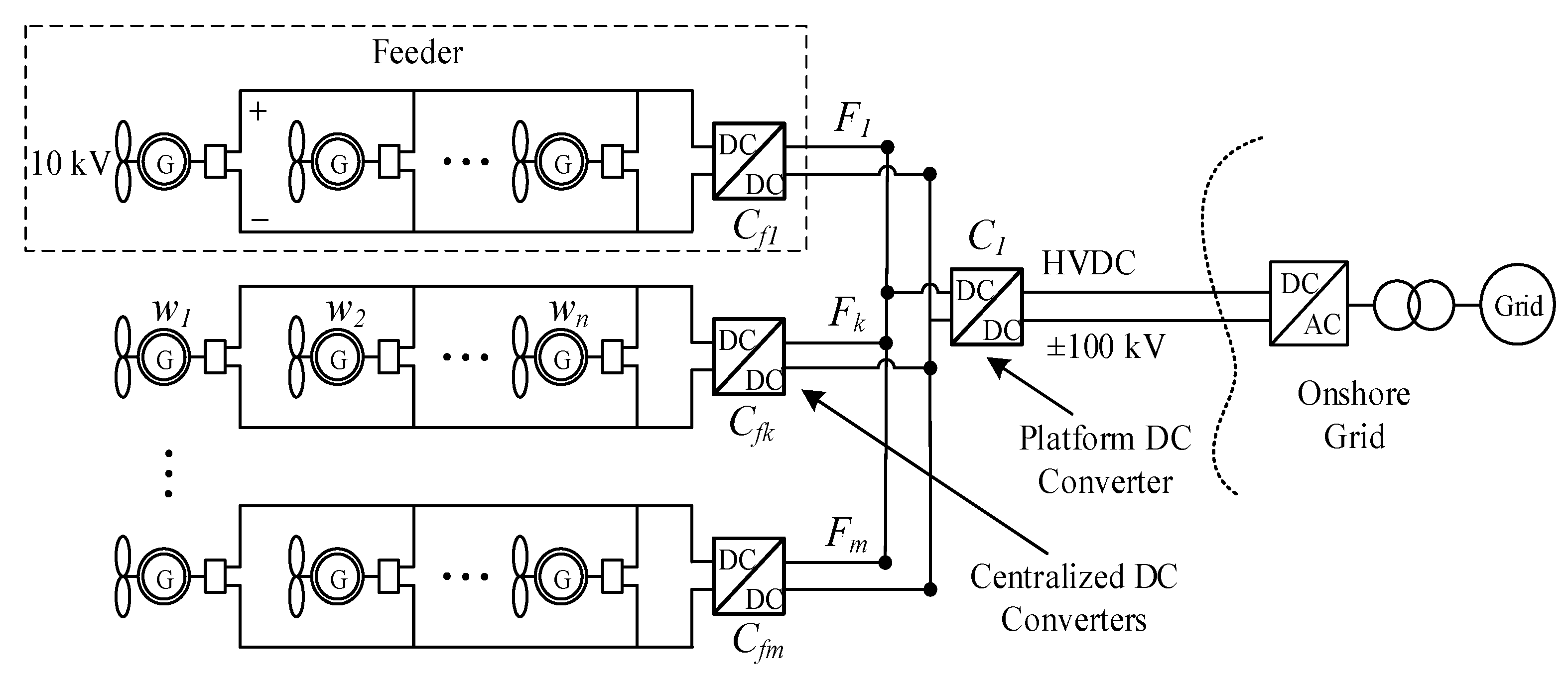
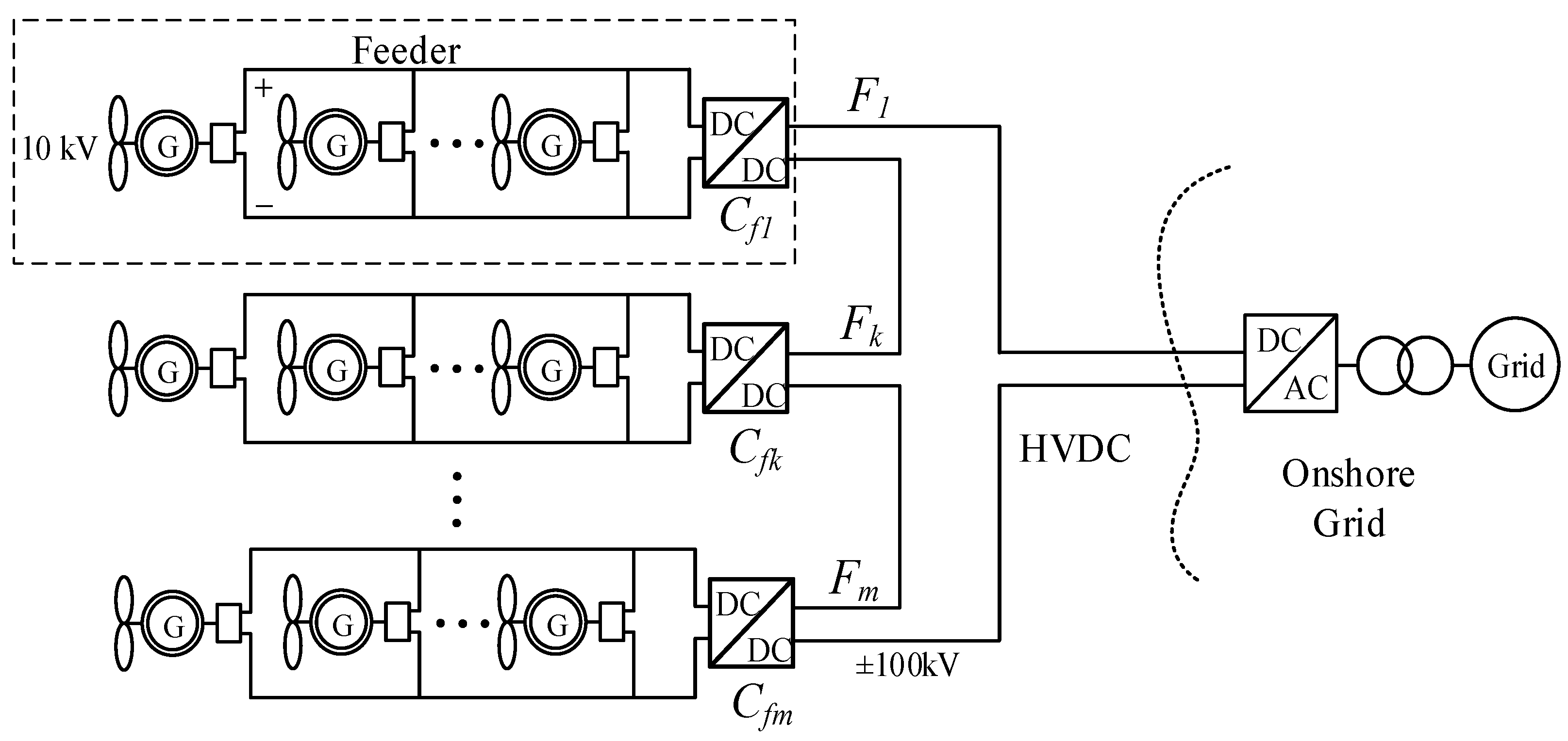
2. Network Topologies for DC Collection Systems

The proposed DC collection system topologies for OWFs include different configurations of radial topology, series topology, series–parallel (SP) topology, and matrix topology [17,19,28]. As shown in Figure 1, Figure 2, Figure 3 and Figure 4, the availability levels of three different configurations of radial topology and SP topology are first analyzed. In this analysis, the MVDC and HVDC pole-to-pole voltage levels were set to ±10 kV and ±100 kV, respectively. The matrix topology is an improved version of the SP topology [28]. However, it uses additional switchgear, which is more complex to control, and the investment is also higher as compared to SP topology, hence opt from this analysis.

2.1. DC Radial Collection Systems

In any radial configuration, at least one centralized DC/DC converter is required to boost the voltage to the HVDC transmission voltage level. The configuration in Figure 1 uses a single collection system platform. The number of WTs connected to each feeder is decided by the optimized network layout under multiple factors, such as the current carrying capacity of cables, network losses, etc. In the radial configuration, the use of a reduced number of voltage conversion stages is beneficial to minimize the capital cost. To improve the reliability of the centralized DC/DC converter station, modular designs can be used [29].
Among the candidate DC/DC converters available for high power applications, the Dual Active Bridge (DAB) converter looks promising in terms of flexibility in power flow control [30,31]. One drawback of this configuration is that it requires a higher voltage gain to boost the voltage from the MVDC level to the HVDC level. However, to overcome this issue, modular designs, such as modular multi-level converter (MMC) with input-parallel, and output-series (IPOS) connections with a lower transformation ratio, can be used at the expense of capital investment [30].
Figure 2 shows a radial configuration that comprises an individual collection system platform per feeder (Radial-2). This topology is more suitable for OWFs, where the centralized collection system platform is located far away from the OWF collection system. Another advantage of this topology is the ability to use lower voltage transformation ratios. The DC output voltage of WTs is first boosted by the intermediate DC/DC converter and then a higher MVDC voltage level than the voltage in Radial-1 topology is used, at the centralized collection system. However, due to the utilization of multiple DC/DC converters, the capital cost is higher than the Radial-1 topology.
The feeder configuration of the Radial-3 topology is shown in Figure 3. This configuration is almost the same as Radial-2, except for the intermediate DC/DC converter voltage levels. In this configuration, the intermediate platforms are connected in series to build up the required HVDC voltage level. One advantage of this topology is the elimination of the platform converter platform, which enables reducing the capital investment. However, the inherent drawbacks of SP topology, which are discussed in Section 2.2, are also associated with this topology.

2.2. Series–Parallel Collection System

In the series or SP topology (Figure 4), the WTs are connected in series to build up the HVDC transmission voltage. However, in the series topology, there is only one feeder/branch and it has a lower wind farm output capacity than the SP topology, hence, it was eliminated from the analysis. The main advantage of SP topology is that it requires no intermediate platforms to boost the voltage to the transmission level. This helps to minimize capital investment.
The main drawback of this topology is that, upon failure of multiple WTs, the healthy units are required to maintain the pole-to-pole HVDC voltage level [32]. However, if the allowable voltage limits are exceeded by individual units (typically 10% of the rated voltage), the entire string is required to implement a forced-shutdown. Further, additional requirements such as (a) proper insulation coordination between each series-connected WT, and (b) special insulation designs for each unit are some other drawbacks of this SP topology.

3. Methodology

The OWF reliability assessment uses two basic techniques—(a) analytical methods, and (b) chronological simulation methods. The analytical methods such as Reliability Block Diagrams (RBDs) [33], Markov processes [34], capacity outage probability tables (COPT) [35], and methods, based on the minimal spanning tree technique [23] were used to evaluate the reliability of OWFs in the literature. The chronological simulation technique called Monte Carlo simulation (MCM) is also a widely used method in the literature [36,37]. The MCM method relies on repeated random samples to obtain numerical results that are computationally inefficient, as compared to analytical methods.
In general, a physical component operates with binary states, i.e., working or failed state, with their associated probabilities. However, due to the stochastic nature of wind speed, the WT power output is always coupled with the probability distribution of the wind. Although the WT is in a healthy operational condition (with a certain probability), its power output always correlates with the corresponding state probabilities of wind speed. Thus, this can be considered to be a multi-state system that is driven by a single source, i.e., wind. In the OWF reliability assessment, the variability of wind speed is required to be incorporated. The established methods based on RBDs or COPT tables to evaluate such systems with a large number of components is inherently complex. To overcome this computational complexity with different network structures and their dependency on external constraints, the proposed UGF technique can be easily adapted. Compared with other analytic methods, the required reliability results can be obtained with a fewer calculation step.
Section 3.1 first introduces the clustering method used to quantify the finite number of wind turbine power output states, with their associated state probabilities. Then, Section 3.2 presents the mathematical representation of the UGF technique as the basis for reliability evaluation. Next, the UGF model is applied to different DC collection system options to evaluate their availability levels, using indices such as GRA and EENS. Finally, a detailed cost model is presented to perform economic analysis.

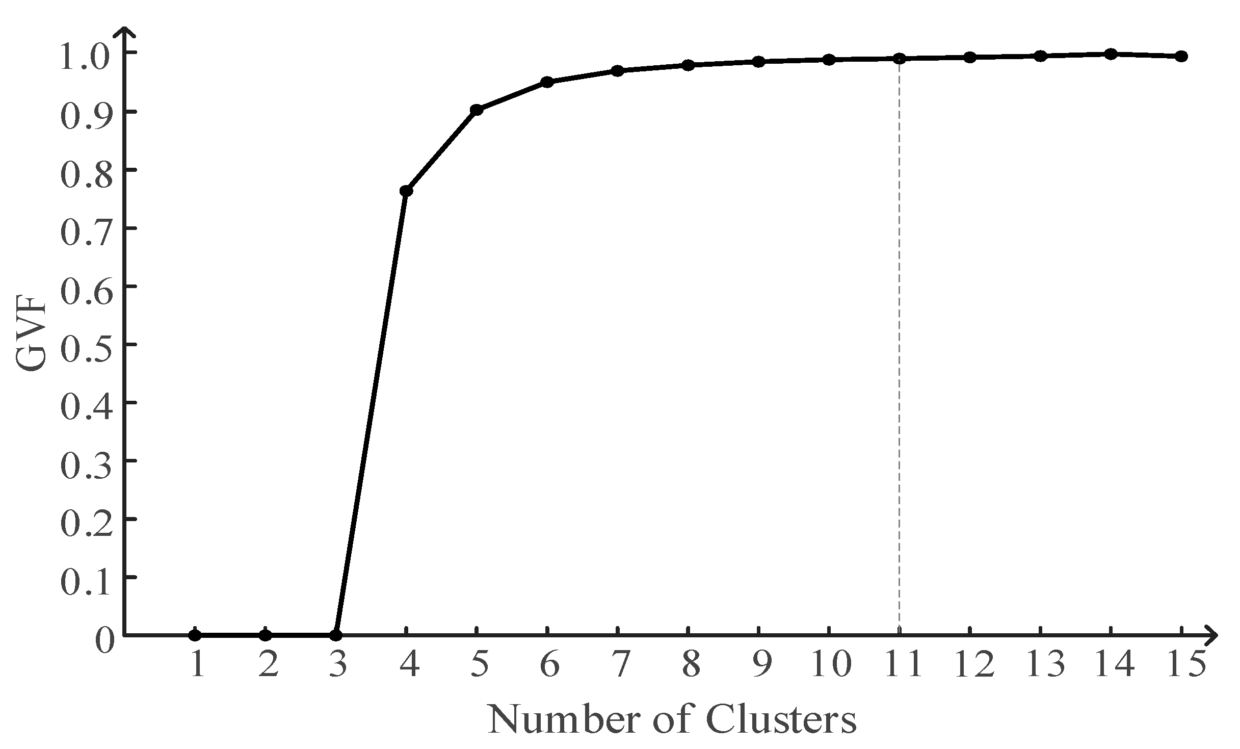
3.1. Clustering of Wind Turbine Power Output

To evaluate OWF reliability, first, it is required to obtain corresponding state probabilities of WT power output from the measured time-series wind speed data (typically between 1–10 min sampling interval) for a certain period (typically 1 year). However, accounting for all state probabilities of time-series data (e.g., 52,560 state probabilities in 10 min average) with very low probabilities, only increases the computational time. Therefore, as shown in Figure 5, the clustering of WT power output into a finite number of states will enhance the computational efficiency when analytical techniques are used.
The intermittent and randomness of wind speed result in different states of WT power output. To obtain the corresponding WT power output for a certain wind speed, it is required to refer to the WT power curve provided by the manufacturer’s datasheet. This is given by:
P w ( v w ) = { 0 v w < v c i P r · ( v w v c i ) ( v r v c i ) v c i v w < v r P r v r v w < v c o 0 v c o v w
where Pw(vw) is the power generated at wind speed vw (m/s), vci is the cut-in wind speed, and vco is the cut-out wind speed. Pr is the rated power of the wind turbine, and vr is the rated wind speed. It can be seen from Equation (1) that the relationship between the instantaneous wind speed and instantaneous power output of WT is non-linear.
Among the different clustering techniques available in the literature, this study used the Jenks Natural Breaks method to quantify the time-series wind power output data into a finite number of states [38,39]. The classification principle of this method is based on grouping similar sized data. The variance of the data is used to measure the classification effect, i.e., to determine the number of clusters. First, it calculates the variance of each category, and then the sum of the variances of all categories are calculated. The smaller the sum of variance, the better the classification effect. Therefore, first, the number of clusters K must be determined. The calculation process for obtaining the objective function i.e., Goodness of Variance Fit (GVF) is mathematically represented by Equations (2)–(4), as follows:
S D A M = 1 N i = 1 N ( z i z ¯ ) 2
S D C M = j = 1 K 1 N j i = 1 N j ( z i j z ¯ j ) 2
G V F = 1 S D C M S D A M
where SDAM (Sum of Squared Deviations from the Array Mean) is the variance of all data, which is a fixed value. N is the number of data, zi is the ith data point, z ¯ is the average value of the data set, SDCM (Sum of Squared Deviations about Class Mean) is the sum of the variances when data are divided into K categories, Nj is the number of data in the jth category, zij is the ith data in the jth category, and z ¯ is the average value of the jth category. SDCM is related to the value of K. SDCM decreases with an increase in K. When K = n, SDCM = 0 and GVF = 1. The larger the GVF, the better the classification effect.

3.2. Reliability Modelling

3.2.1. Failure Rate Calculation of dcWT

The dcWT used in this analysis can be considered to be an extension of Type-4 acWT, which replaces the grid side converter (GSC) with a DAB DC/DC converter [19]. The operating status of the WT is determined by the availability of each sub-system, such as the generator, converter, gearbox, etc. It was assumed that all components were independent and hold Markov properties [40]. In the Markovian context, the status of a component/sub-system was represented by the binary state-space model, as shown in Figure 6.
The average failure λ ¯ and repair rate μ ¯ of the dcWT can be calculated using Equations (5) and (6), with the knowledge of its subsystems as follows:
λ ¯ = i = 1 r λ i
μ ¯ = λ ¯ i = 1 r λ i μ i 1
where λi and μi are the failure and repair rates of the dcWT ith sub-system, which has r number of total sub-systems. The availability AWT of the whole system, i.e., the probability of being in the working state can be calculated as Equation (7), and the unavailability level UWT is defined as Equation (8):
A W T = μ ¯ λ ¯ + μ ¯
U W T = λ ¯ λ ¯ + μ ¯

3.2.2. The Universal Generating Function

Suppose there are n discrete random vectors G1, G2, G3, …, Gn, where the probability distribution of Gi can be represented by two vectors gi and pi. The vector gi represents the possible value of Gi and the vector pi represents the probability corresponding to the value of Gi:
g i = { g i , 1 , g i , 2 , g i , 3 , , g i , m i } p i = { p i , 1 , p i , 2 , p i , 3 , , p i , m i }
where:
p i , j = Pr { G i = g i , j }           j = 1 , 2 , , m i
For a random variable Gi, the polynomial form of its z-transformation is defined as:
U i ( z ) = p i , 1 z q i , 1 + p i , 2 z q i , 2 + + p i , m i z q i , m i = j = 1 m i p i , j z q i , j
where z is just a symbolic notation. The index qi,j represents the value of the variable, and the coefficient pi,j represents the probability when the variable value is qi,j. Therefore, the z- transformation for the system consisting of n random variables can be represented as:
U ( z ) = f ( U 1 ( z ) , U 2 ( z ) , , U n ( z ) ) = f ( j 1 = 1 m 1 p 1 , j 1 z q 1 , j 1 , j 2 = 1 m 2 p 2 , j 2 z q 2 , j 2 , , j n = 1 m n p n , j n z q n , j n ) = j 1 = 1 m 1 j 2 = 1 m 2 j n = 1 m n ( i = 1 n p i , j i z f ( q 1 , j 1 , q 2 , j 2 , , q n , j n ) )
where U(z) is the UGF of the function and f is the combination operator of UGF. For instance, if the system contains two components in series, the UGF of the system is given by:
U ( z ) = f ( U 1 ( z ) , U 2 ( z ) ) = j 1 = 1 m 1 j 2 = 1 m 2 ( i = 1 n p i , j i z min ( q 1 , j 1 , q 2 , j 2 ) )
Thus, the f combination operator is the minimum value of (q1 and q2) of system variables under the governing constraints. Similarly, for a system with two components in parallel, the UGF can be represented as Equation (14), where the combination operator is the addition of (q1 and q2).
U ( z ) = f ( U 1 ( z ) , U 2 ( z ) ) = j 1 = 1 m 1 j 2 = 1 m 2 ( i = 1 n p i , j i z q 1 , j 1 + q 2 , j 2 )

 UGF Model for Radial Topology 

In the radial topologies presented in Figure 1, Figure 2 and Figure 3, assume that there are n WTs per feeder and m total number of feeders. Consider the states of the WT as operating at power level Px MW or failed state, i.e., 0 MW with corresponding state probabilities p1 and p2 (=1 − p1), respectively. For the time being, assume that the probability of power output level Px is px = 1. The UGF of the ith WT Ui(z, x) can then be represented by:
U i ( z , x ) = p 1 z P x + p 2 z 0
For n WTs in parallel, the UGF function for kth feeder UFk is represented by:
U F k ( z , x ) = ( U 1 ( z ) , U 2 ( z ) , , U i ( z ) , , U n ( z ) ) = i = 1 n ( p 1 z P x + p 2 z 0 ) i = ( p 1 z P x + p 2 z 0 ) n = a 0 z 0 + a 1 z P x + a 2 z 2 P x + + a i z i P x + + a n z n P x
Define the UGF of the platform DC/DC converter C1 with the corresponding state probabilities of perfect functioning as pc1 and failure as pc2 by:
U C 1 = p c 1 z n m P x + p c 2 z 0
Similarly, the UGF of the kth centralized DC/DC converter CFk (k = 1,2, … k, …, m) with corresponding state probabilities of perfect functioning as pcf1 and failure as pcf2 is defined as:
U CF k = p c f 1 z n P x + p c f 2 z 0
  • Radial-1 Topology
As shown in Figure 1, all MVDC feeders are aggregated at the platform DC/DC converter in Radial-1 topology. The UGF of the OWF collection system Ur1, which has n × m number of WTs can be defined as:
U r 1 ( z , x ) = ( U F 1 ( z ) , U F 2 ( z ) , , U F k ( z ) , , U F m ( z ) ) = ( k = 1 m ( p 1 z P x + p 2 z 0 ) n k = b 0 z 0 + b 1 z P x + b 2 z 2 P x + + b i k z i k P x + + b n m z n m P x
Next, to obtain the UGF of the Radial-1 topology, the UGFs of the collection system and the platform DC/DC converter is combined using the formula:
U R a d i a l 1 ( z , x ) = min ( U r 1 ( z , x ) , U C 1 ( z , x ) ) = ( b 0 z 0 + b 1 z P x + b 2 z 2 P x + + b i k z i k P x + + b n m z n m P x ) × ( p c 1 z n m P x + p c 2 z 0 ) = ( p c 1 b 0 z min ( 0 , n m P x ) + p c 2 b 0 z min ( 0 , 0 ) + p c 1 b 1 z min ( P x , n m P x ) + p c 2 b 1 z min ( P x , 0 ) + p c 1 b 2 z min ( 2 P x , n m P x ) + p c 2 b 2 z min ( 2 P x , 0 ) + + p c 1 b i k z min ( i k P x , n m P x ) + p c 2 b i k z min ( i k P x , 0 ) + + p c 1 b n m z min ( n m P x , n m P x ) + p c 2 b n m z min ( n m P x , 0 ) ) = ( c 0 z 0 + c 1 z P x + c 2 z 2 P x + + c i k z i k P x + + c n m z n m P x )
In Equation (20) the combination operator f is the minimum value of corresponding to the state variables. Finally, the UGF of the Radial-1 topology for Px power, which corresponds to cluster x with the state probability of pwt_x can be obtained as:
U R a d i a l 1 ( z , x ) = p w t _ x × ( c 0 z 0 + c 1 z P x + c 2 z 2 P x + + c i k z i k P x + + c n m z n m P x )
Considering that all ncl WT power output clusters, the UGF of the Radial-1 topology is given by:
U G F O W F R a d i a l 1 = x = 1 n c l U G F R a d i a l 1 ( z , x )
  • Radial-2 Topology
Similarly, using Equations (16) and (18), the UGF of a feeder in Radial-2 topology which combines the n parallel WTs, and the centralized DC/DC converter could be represented as:
U C F k ( z , x ) = min ( U F k ( z , x ) , U C F k ( z , x ) ) = ( a 0 z 0 + a 1 z P x + a 2 z 2 P x + + a i z i P x + + a n z n P x ) × ( p c f 1 z n P x + p c f 2 z 0 ) = ( p c f 1 a 0 z min ( 0 , n P x ) + p c f 2 a 0 z min ( 0 , 0 ) + p c f 1 a 1 z min ( P x , n P x ) + p c f 2 a 1 z min ( P x , 0 ) + p c f 1 a 2 z min ( 2 P x , n P x ) + p c f 2 a 2 z min ( 2 P x , 0 ) + + p c f 1 a i z min ( i P x , n P x ) + p c f 2 a i z min ( i P x , 0 ) + + p c f 1 a n z min ( n P x , n P x ) + p c f 2 a n z min ( n P x , 0 ) ) = ( d 0 z 0 + d 1 z P x + d 2 z 2 P x + + d i z i P x + + d n z n P x )
Following Equation (19), m-feeders of the Radial-2 topology can be combined as follows:
U r 2 ( z , x ) = ( U F 1 ( z ) , U F 2 ( z ) , , U F k ( z ) , , U F m ( z ) ) = ( k = 1 m ( d 0 z 0 + d 1 z P x + d 2 z 2 P x + + d i k z i P x + + d n m z n P x ) k = e 0 z 0 + e 1 z P x + e 2 z 2 P x + + e i k z i k P x + + e n m z n m P x
Finally, to obtain the UGF of the Radial-2 topology, the UGFs of the collection system and the platform DC/DC converter could be can using Equation (20). The final UGF is obtained using Equations (21) and (22).
  • Radial-3 Topology
In Radial-3 topology, the UGF of the OWF collection system is the same as in the Radial-2 topology defined in Equation (23). However, the feeders are connected in series, in which its topology reliability can be considered as a k-out-of-n(G) system. The OWF remains connected to the grid until n – k + 1 feeder DC/DC converters fail. The value of k is decided by the allowable over-voltage limit of each DC/DC converter. The technique used to obtain the UGF of a general k-out-of-n(G) system in [27] was adapted with necessary modifications.
  • Determine the UGF (UCFk) of each feeder DC/DC converter as in Equation (18)
  • Obtain the UGF of all m feeders (k = 1,2,…,m)
    U C F ( z , x ) = ( U C F 1 ( z ) , U C F 2 ( z ) , , U C F k ( z ) , , U C F m ( z ) ) = ( k = 1 m ( p c f 1 z n P x + p c f 2 z 0 ) k = f 0 z 0 + f 1 z n P x + f 2 z 2 n P x + + f k 1 z ( k 1 ) n P x + f k z k n P x + + f m z m n P x
  • Define the value of kmin, i.e., the minimum number of centralized DC/DC converters required for a successful operation of the OWF collection system.
  • Obtain the new UGF by replacing all zknPx with z0 for k < kmin in Equation (25)
    U C F ( z , x ) = f 0 z 0 + f 1 z 0 + f 2 z 0 + + f k 1 z 0 + f k z k n P x + + f m z m n P x = ( f 0 + f 1 + f 2 + + f k 1 ) z 0 + f k z k n P x + + f m z m n P x
  • Finally, combine Equation (26) with the UGF of the OWF collection system Ur1, which comprises m-feeders and n-WTs per feeder, as defined in Equation (19).
    U r 3 ( z , x ) = min ( U C F ( z , x ) , U r 1 ( z , x ) ) = ( ( f 0 + f 1 + f 2 + + f k 1 ) z 0 + f k z k n P x + + f m z m n P x ) × ( b 0 z 0 + b 1 z P x + b 2 z 2 P x + + b i k z i k P x + + b n m z n m P x ) = g 0 z 0 + g 1 z P x + g 2 z 2 P x + + g i k z i k P x + + g n m z n m P x
  • The final UGF for ncl states can be obtained by referring to Equations (21) and (22).

 UGF Model for Series-Parallel Structure 

In SP topology, WTs are connected in series to build up a feeder and then the feeders are connected in parallel. Consider a feeder as a subsystem here. In this subsystem, when a single WT fails and is by-passed, the pole-to-pole voltage of the feeder must still be within the allowable voltage limits. However, the terminal voltages of healthy WTs increase to match the pole-to-pole voltage of the entire string. In this situation, if multiple WTs trip, healthy units experience overvoltages at their terminals beyond their maximum limits. Thus, as a safety measure, the entire feeder is required to implement a forced shutdown. Therefore, a feeder in the SP topology can be considered as a k-out-of-n(G) system.
Consider the feeder-F1 in Figure 4 where n WTs are connected in series per feeder and there are m feeders in parallel. Assuming the power output of WTs is aggregated into ncl clusters, the UGF of the feeder at the xth state can be represented as:
U G F F 1 ( z , x ) = i = 0 n k C n i p 1 ( n i ) p 2 i z P x × ( n i ) + i = n k + 1 n C n i p 1 n i p 2 i z 0 x = 1 , 2 , , n c l
where all variables are denoted as in Section 3.2.2. Assuming the negligible impact of the wake effect, the UGF of SP topology with m-parallel feeders can be defined as:
U G F S P ( z , x ) = p w t _ x × f ( U G F F 1 ( z , x ) , U G F F 2 ( z , x ) , , U G F F m ( z , x ) ) = p w t _ x × U G F F 1 ( z , x ) × U G F F 2 ( z , x ) × × U G F F m ( z , x ) = a 0 z 0 + a 1 z P x + a 2 z 2 P x + + a n m z n m P x
where pwt_x is the probability of Px being in the xth state. Finally, considering all ncl cluster states, the UGF of SP topology can be obtained as follows.
U G F O W F _ S P ( z , x ) = x = 1 n c l U G F S P ( z , x )

3.2.3. Reliability Indices

To evaluate the associated availability levels of different DC collection systems, the Expected Energy Not Supplied (EENS) and Generation Ratio Availability (GRA) [41] are used. The EENS is the energy the system that is not able to export to the point of connection due to probabilistic uncertainties of the system. This can be expressed as:
E E N S = i = 1 N p i × ( P O W F max P O W F i ) × 8760
where pi is the probability that the whole system is in the ith power output state, POWFmax is the rated capacity of the OWF, POWFi is the power output of the whole system in the ith state. The total number of states N is the product of the number of WTs nwt and the number of WT power output clusters ncl.
The GRA refers to the probability of at least a certain percentage (defined as Generation Ratio Criterion-GRc) of electrical energy that could be delivered to the grid. Let the column matrix V be defined by:
V = [ V 1 V 2   V x   V n c l ] n c l × 1 ; x = 1 , 2 , , n c l
where Vx = [a0, a1, a2,..., anm] is a row matrix with a0, a1, a2,..., anm that denotes the corresponding state probabilities of the respective collection system and remains in a certain power output level Px. GRA(GRc) represents the ratio of power generation availability under the condition of at least i working wind turbines:
G R A ( G R c ) = j = 2 n c l h = i n m V ( j , h ) ; G R c = i n × m × 100 %

3.3. Lifetime Cost Estimation

When identifying a suitable DC collection system option for an OWF, life-cycle costs of candidate topologies are required to be considered. Cost estimation is as important as reliability evaluation. To fully reflect the economics of different topologies, both the initial investment costs and costs incurred due to network losses during its operational lifecycle is incorporated. The initial investment cost mainly includes the cost of WTs, cables, and converters, while the costs associated with operational losses mainly include the cables and converter losses.

3.3.1. Capital Investment

  • WT Cost
The dcWT concept is still at the research and development stage. Therefore, the capital cost was estimated, based on the available prices for acWTs of the same rated capacity, with required modifications. A detailed cost-breakdown of different components for a fully-rated, power-converter-based offshore acWT (Type-4) could be found in [42]. As discussed in Section 2.1, a DAB-based dcWT topology was considered in this analysis. This could be considered as an addition of an AC/DC converter to the acWT front-end, and the cost of AC/DC converter was 8667.4 £/MW. The required capital costs of 10 MW, 8 MW, and 5 MW dcWTs are shown in Table 1.
  • DC/DC Converter Costs
The capital cost per unit capacity (£/MW) of a centralized DC/DC converter and platform DC/DC converter was different, due to various techno-economic factors. The cost of the centralized and the platform DC/DC converters were taken as 120 £/kVA [43], and 0.22 M£/MW [44], respectively.
  • DC Cable Cost
To calculate the capital cost of DC cables with different current carry capacities, the following formula was considered, as discussed in [44,45]:
C c a b l e = R a t e × ( A + B P n ) × l c a b l e P n = U n I n
where Pn is the rated power of the cable (W), Un is the rated pole-to-pole DC voltage of the cable (V), and In is the rated current of the cable (A). The term Rate is the exchange rate of Swedish krona to the British pound, lcable is the cable section length (km), and A and B are coefficients shown in Table 2.

3.3.2. Costs Associated with Energy Losses

  • Cable Losses (Radial Topology)
The current flow of a radial WT feeder is shown in Figure 7. Notably, the upstream cable sections were required to carry more currents than the downstream sections.
The total power loss for a certain rated current I (kA) can be obtained as follows [46]:
P l o s s c a b l e = ( I 2 + ( 2 I ) 2 + ( 3 I ) 2 + + ( n I ) 2 ) R c a b l e I = P w ( v w ) U c a b l e R c a b l e = R l c a b l e
where R is the cable resistance for a unit length (Ω/km), and lcable is the cable length (km), as shown in Figure 7. The distance between the wind turbines in the same feeder and adjacent feeders were set to 9D, where D denotes respective rotor diameters of WTs [47,48].
  • Cable Losses (SP Topology)
In SP topology, the current flowing through each section along the feeder was the same. Therefore, to obtain the cable losses of the SP topology Equation (35), the following modification could be used:
P l o s s c a b l e = ( I 2 + I 2 + + I 2 ) R c a b l e
  • Converter Losses
Converter losses include both the centralized DC/DC converter and platform DC/DC converters. The required converter losses with different MVDC voltage levels and power levels were obtained using the PLECS simulations. The work in [49] could be used to calculate these losses.
  • Cost of Losses
The total annual energy losses of each DC collection system Eloss can be obtained by:
E l o s s = t s T ( P l o s s c a b l e + P l o s s c o n v e r t e r ) t s
where Ploss-cable is the time-varying losses of DC cables that changes with wind speed and ts is the corresponding sampling time, i.e., wind speed measurement interval. The term T is the total period considered (typically one year). Finally, the cost of losses during the life cycle Closs can be obtained as follows:
C l o s s = E l o s s × e n e r g y   p r i c e i ( 1 1 ( 1 + i ) T l i f e )
where i denotes the annual interest rate and Tlife is the average life of an OWFs.

4. Case Study

4.1. Obtaining Optimal Number of Wind Power Output Clusters and Other Parameters

As discussed in Section 3, first it is required to obtain an optimal number of wind power output clusters with their corresponding state probabilities. Initially, the time series wind speed data is converted to corresponding power output using Equation (1). In this analysis, 10-min average wind speed data available with FINO2 offshore weather station is used [50]. Table 3 summarizes the nameplate data for selected WTs, with their capacities for three scenarios 10 MW (S1), 8 MW (S2), and 5 MW (S3). It is worth noting that the nameplate data provided in Table 3 were obtained from commercially available acWTs. They were used to refer to the corresponding power curves of dcWTs with the same capacity and to define the inter-turbine distances.
Using the Jenks Natural Breaks clustering method, the WT power output for each rated capacity was clustered into a finite number of states. The optimum number of clusters were selected with the objective function value, which is defined as GVF in Equation (4). Figure 8 illustrates the corresponding GVF values for different number of clusters for 10 MW dcWT.
Notably, for this time-series data set, the GVF difference between adjacent clusters was less significant after 11 clusters. Therefore, 11 clusters were selected to represent the stochastic behavior of the WT output. Table 4 summarizes the cluster center values with their corresponding state probabilities for 10 MW dcWT.
The failure and repair rates of different sub-assemblies of typical offshore WT is considered and summarized in Table 5 [54]. The failure rate of the DC/DC converter was obtained using the methodology presented in [49]. Notably, compared to other sub-assemblies, the failure rates of power converters were relatively higher due to the greater intrinsic failures of semiconductor devices. The availability level of 98% was considered for the platform DC/DC converters in complying with the specified availability levels of Crown Estate licensed offshore wind farms around the UK [55].
To calculate the accumulated energy losses for different topologies, losses of DC/DC converters are required to be considered, as they are one of the key building blocks of the DC collection systems. The total switching and conduction losses of the DC/DC converters at different MVDC voltage levels and power levels are required to be first calculated. The accumulated energy losses of different topologies were obtained through PLECS simulation and are shown in Table 6. The notations R-1,2,3 denote the radial topologies shown in Figure 1, Figure 2 and Figure 3, with their corresponding DC/DC converters C1 and Cf1.

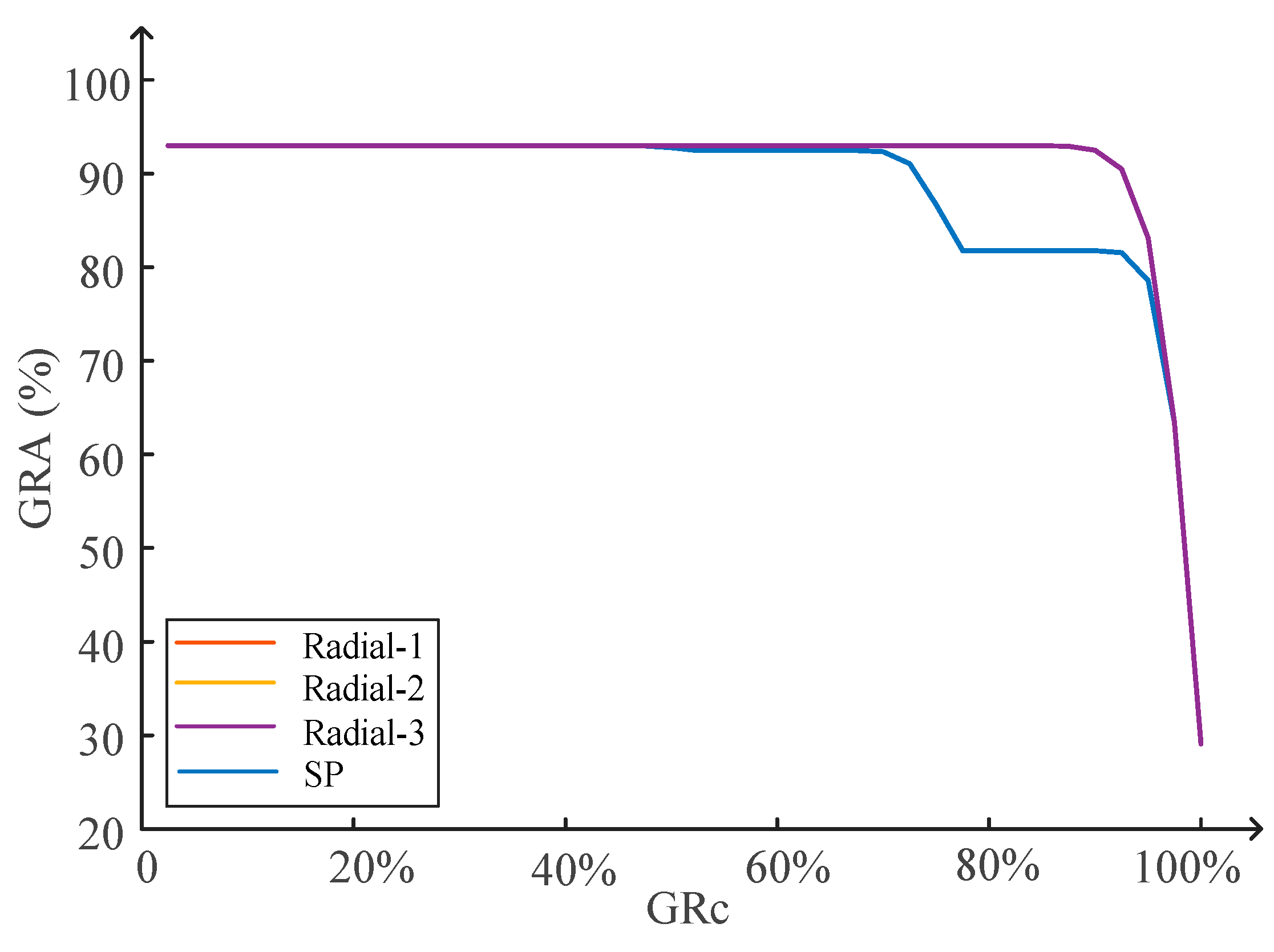
4.2. Reliability of DC Collection Systems

In general, EENS and GRA indices are used to evaluate reliabilities for different DC collection system options, which do not depend on load demand at the point of common coupling. It can be seen from Figure 9 that irrespective of the topology, the larger the WT capacity, the larger the EENS. This is because the failure of a single WT with a higher rated power loses more energy as compared to a smaller WT that has the same failure probability. Among all four topologies, the Radial-3 configuration accounts for the largest EENS, whereas the Radial-1 topology shows the lowest for all the three WT scenarios.
Notably, for the 8 MW and 5 MW cases for Radial-1,2, and SP topologies, the EENS difference was about 0.1%. In this analysis, the same number of WTs (i.e., 10 WTs per feeder) was used for all scenarios, irrespective of the WT capacity. Therefore, the use of the same failure rates for each case results in lower EENS for lower WT capacity. This is one possible reason for this negligible EENS difference between the 8 MW and 5 MW cases.
The GRA for the whole range of GRc (from 1% to 100%) for all topologies of 10 MW (S1) is shown in Figure 10. At higher GRc levels, the Radial-1 topology provides higher availability levels than the other three topologies. For instance, at GRc (90%), the Radial-1 topology shows a 90.6% availability level, followed by Radial-3 with 85.3%. The SP topology shows the lowest with an 81.8% availability level. It is worth noting that for the same GRc, different topologies represent different GRA levels. This is because, at the same GRc of 90%, S1, S2, S3 requires at least 36, 45, and 72 WTs to be in healthy operating conditions, respectively. Thus, their state probabilities are different, and the availability levels vary, depending on the configuration.
Although the Radial-3 topology shows the second-highest availability level at GRc of 90%, until GRc of 75.4%, it shows the lowest availability level among the four topologies, making it the least reliable.
Figure 11 illustrates the GRA variation for different availability criterion related to 8 MW (S2) and 5 MW (S3) WT Cases. Similar to the previous case (S1), the GRA variation of S2 in Figure 11a shows a similar pattern. However, the GRA of Radial-3 topology remained the lowest at GRA of 82.3%, until GRc up to 79.9%. At GRc of 90%, Radial-1 topology showed an availability level of 89.1%, which was 1.5% lower compared to S1.
Notably, for the S3 case until GRc of 73%, all the DC collection system options showed a similar GRA of about 90%, as shown in Figure 11b. This is because when the number of system components increases, it requires a relatively higher number of WTs to remain in a healthy operation condition at lower availability levels, as compared to cases S1 and S2. However, at higher GRc levels, failure of multiple WTs (to maintain the same availability ratio) will result in lower GRA values under the same WT failure rates. In this case, at GRc of 90%, Radial-1, 2, and 3 topologies showed 89.3%, 75.9%, and 77.5% GRA levels. Similar to other cases, SP topology showed the lowest availability level with 70.4%.
To observe the variation of GRA with different WT capacities with the available data, this study considered the same WT failure rate for all cases. As shown in Figure 12 when all DC/DC converters were failure-free, the GRA variation of Radial-1, 2, 3 was the same, since the collection system configuration was radial. This also highlighted the importance of maintaining higher availability levels of DC/DC converters located at different positions, for each radial configuration. However, the SP topology showed a different variation, since the WT connection was different.

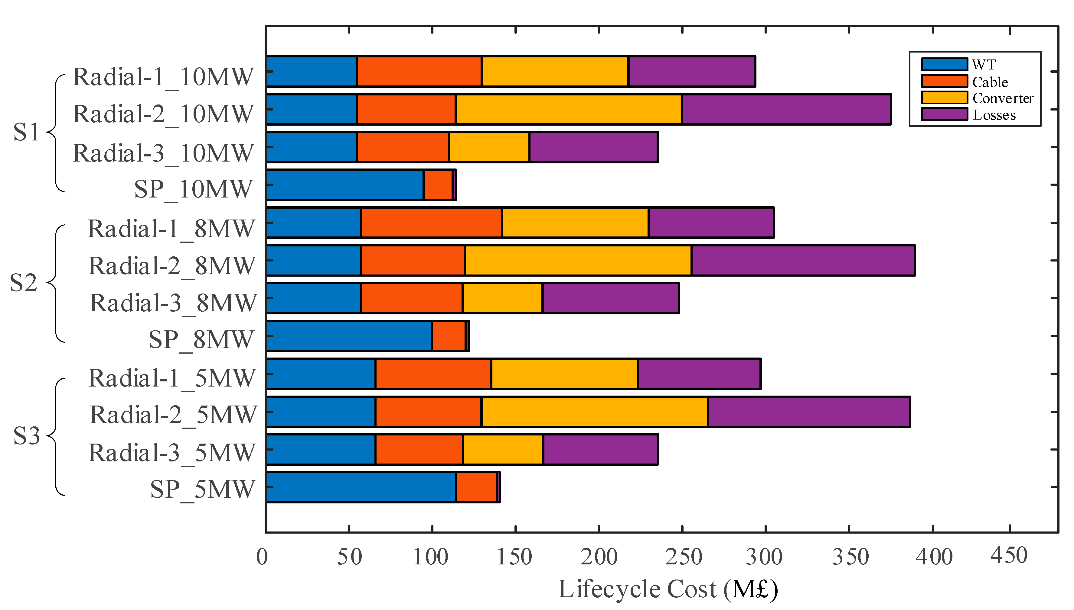
4.3. Economic Evaluation of Candidate DC Collection Systems

To assess the economies of scale of different candidate DC collection systems, the capital and operational costs of each topology were calculated, based on the methodology discussed in Section 3.3. As shown in Figure 13, the capital cost included WT cost, cable cost, and converter cost, and the operational losses included cable- and converter-losses. For this analysis, the average lifetime of the offshore wind farm was considered as 25 years [56] and for electrical energy losses calculations, the energy price of 75 £/MWh [18] with a discount rate of 5% was considered [49].
Among the four topologies, the total cost of SP topology was significantly lower than other topologies, due to the elimination of the centralized DC/DC converter. For instance, this cost was about 34% of the lifetime cost of the Radial-1 configuration (S1), which showed better availability. The Radial-2 configuration showed the highest lifetime cost due to the higher capital cost of converters and system losses. For 10 MW and 8 MW dcWT capacities of Radial-1 configuration, the lifetime cost difference was about 11.2 M£.

4.4. Overall Assessment of DC Collection System Options

As discussed above, reliability and lifecycle costs need to be considered to identify a suitable DC collection system option. Figure 14 below summarizes the three functional factors used to determine the reliable and cost-effective DC collection system option, according to the methodology presented. The ideal topology should be the one with the highest GRA, as well as the lowest EENS and lifecycle cost. However, identifying the best topology is not straightforward, due to the inherent characteristics of different topologies.
For example, in SP topology, although the capital investment is lower, its GRA is relatively low, as compared to other radial configurations. Among the three radial configurations, Radial-1 shows the highest GRA with lower EENS for different WT capacities. Hence, it could be considered to be a suitable option for future DC collection systems.

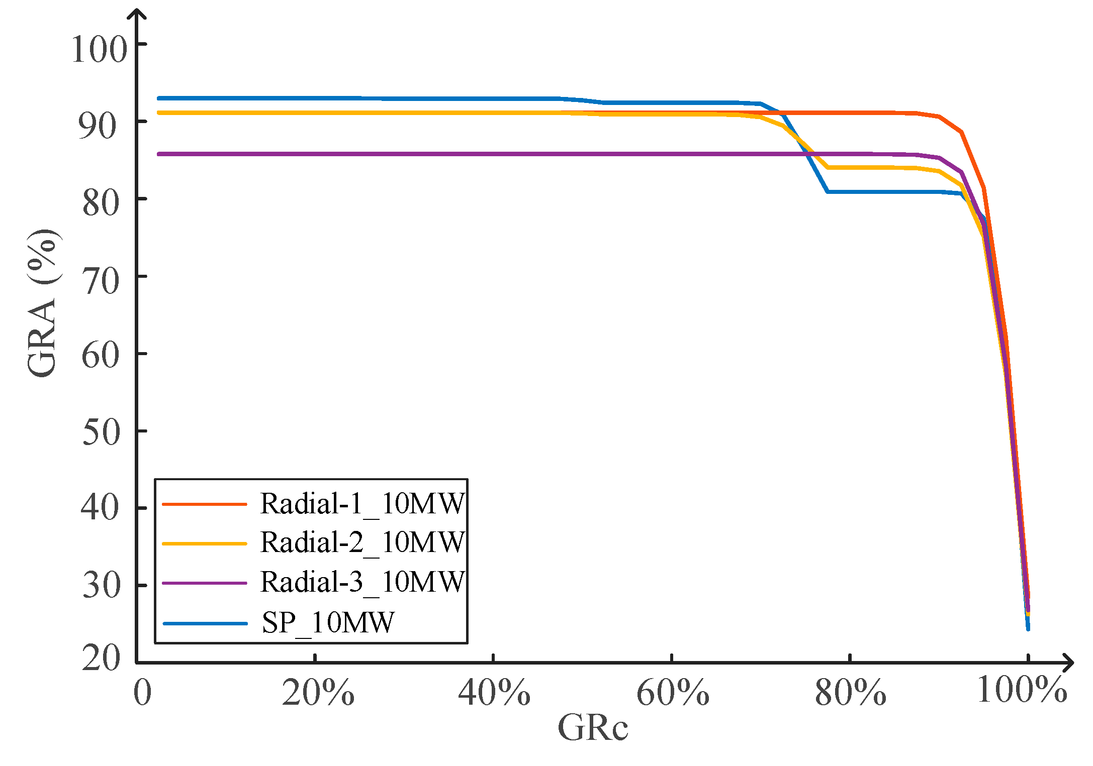
4.5. Impact of the DC Voltage Level for the Reliability of Series–Parallel Topology

Although the SP topology does not qualify as a suitable option with the parameters used in the analysis, a sensitivity analysis was performed to assess its GRA variation and EENS with different terminal voltage levels. As summarized in Table 7, the dcWT terminal voltage was changed from ±2.5 kV to ±25 kV. This resulted in a different number of series-connected dcWTs per feeder. However, the HVDC pole-to-pole voltage level remained unchanged at ±100 kV. Notably, the ±2.5 kV with 40 WTs connected in series was a special case, as it contained a single feeder. This could be considered as the series topology.
According to Table 7, the EENS increased as the terminal DC voltage level increased, which is not favorable. However, in some cases, the use of a higher DC voltage level results in relatively lower EENS than the use of a lower DC voltage level. For instance, consider the ±20 kV and ±25 kV cases that connects 5 and 4 WTs in series. In this case, the use of ±25 kV was economical, since it had a lower EENS of 52,600 MWhr/yr, as compared to ±20 kV case. This was because, for both cases, if a single WT failed, the entire feeder was forced into shut-down; whereas in the ±25 kV case, it contained 10 parallel feeders, making it more reliable than the ±20 kV case with 8 feeders.
Similarly, the GRA variations illustrated in Figure 15 shows better availability levels at higher DC voltage levels, for the same reason as discussed above. However, the use of a lower DC voltage level with a higher number of series-connected dcWTs could provide higher availability levels. For instance, at GRc of 90%, the GRA of ±2.5 kV, ±10 kV, and ±12.5 kV were 92.5%, 81.8%, and 83.8%, respectively.

4.6. Discussion of the Results

In the case study presented above, three different WT capacities were used to observe the variation of reliability and economic factors with different DC collection systems. The results suggest that with an increase in dcWT capacity, the GRA of the collection systems increased. Although SP topology showed a significantly lower lifecycle cost, the reliability was relatively low due to its series-connected network structure over the other radial topologies. Since there are no DC collection systems under operation at present, several assumptions were made when conducting this study. For instance, the failure rates and costs of components such as dcWT, platform DC/DC converters were calculated by referring to the relevant literature. The sensitivity analysis conducted to observe the impact of the reliability of DC/DC converters on the overall availability levels of the collection systems, revealed the requirement to pay higher attention to improve their reliability levels. However, with field experience and technology advancements, the reliability can be improved, although the high-power DC/DC converter technology is still not mature.

5. Conclusions

A potential option in future offshore wind power development is to use DC technology at the collection system. To make the correct investment decision, the selection of a suitable offshore wind farm collection system topology is vital at its initial planning phase. This study aimed to evaluate the reliability and associated lifecycle costs of DC collection system options. Three radial and series–parallel DC collection system configurations were assessed for a 400 MW offshore wind farm. Each had three different DC wind turbine capacity sizes.
An analytical reliability evaluation method called universal generating function (UGF) is proposed to evaluate different reliability indices for these DC collection system options. The use of the UGF technique can greatly improve calculation efficiency for larger systems. An economic model was also accounted for, to consider the initial investment cost and cost of network losses during the operational life.
The results showed that the Radial-1 topology is more reliable than the other three topologies, with the smallest EENS and the largest GRA. On the other hand, the Radial-3 topology is the least reliable option, although it eliminates the centralized collection system platform. Notably, with an increase of DC wind turbine capacity, the GRA (which used to measure the availability levels of these candidate collection system options) increases. In terms of lifecycle cost, the series–parallel topology is the optimal choice, and its lifecycle cost decreases with the increase of the WT capacity. Nonetheless, at higher availability criterion, its reliability is less competitive than the radial topologies.

Author Contributions

Conceptualization, G.A. and J.L.; Data curation, G.A.; Formal analysis, R.S.; Investigation, G.A. and R.S.; Methodology, G.A. and R.S.; Software, R.S.; Supervision, J.L., K.W.; Validation, R.S. and G.A.; Writing—original draft, R.S.; Writing—review & editing, G.A. All authors have read and agreed to the published version of the manuscript.

Funding

This work was supported by the European Commission’s Horizon 2020 Research & Innovation Program (Marie Skłodowska-Curie Actions) through the project “Innovative Tools for Offshore Wind and DC Grids (InnoDC)”, under grant agreement no. 765585 and State Key Laboratory Open Fund Project no. FXB51201901458.

Institutional Review Board Statement

Not applicable.

Informed Consent Statement

Not applicable.

Conflicts of Interest

The authors declare no conflict of interest.

References

  1. UK Becomes First Major Economy to Pass Net-Zero Emissions Law. Available online: https://www.gov.uk/government/news/uk-becomes-first-major-economy-to-pass-net-zero-emissions-law (accessed on 10 February 2021).
  2. European Union. Going Climate-Neutral by 2050: A Strategic Long-Term Vision for a Prosperous, Modern, Competitive and Climate-Neutral EU Economy; Technical Report; European Union: Brussels, Belgium, 2019. [Google Scholar]
  3. Mallapaty, S. How China could be carbon neutral by mid-century. Nature 2020, 586, 482–483. [Google Scholar] [CrossRef] [PubMed]
  4. Ritchie, H.; Roser, M. How Much of Our Primary Energy Comes from Renewables? Available online: https://ourworldindata.org/renewable-energy (accessed on 15 February 2021).
  5. Wang, Q.; Yu, Z.; Ye, R.; Lin, Z.; Tang, Y. An Ordered Curtailment Strategy for Offshore Wind Power under Extreme Weather Conditions Considering the Resilience of the Grid. IEEE Access 2019, 7, 54824–54833. [Google Scholar] [CrossRef]
  6. Global Wind Energy Council. GWEC Global Wind Report 2019; Technical Report; Global Wind Energy Council: Brussels, Belgium, 2019. [Google Scholar]
  7. Global Wind Energy Council. Global Offshore Wind Report 2020; Technical Report; Global Wind Energy Council: Brussels, Belgium, 2020. [Google Scholar]
  8. News Release from Vestas Wind Systems A/S. Vestas Launches the V236-15.0 MW to Set New Industry Benchmark and Take Next Step towards Leadership in Offshore Wind. Available online: https://www.vestas.com/en/media/company-news?n=3886820 (accessed on 16 February 2021).
  9. Skopljak, N. 14 MW GE Haliade-X for Third Phase of World’s Largest Offshore Wind Farm. December 2020. Available online: https://www.offshorewind.biz/2020/12/18/14-mw-ge-haliade-x-for-third-phase-of-worlds-largest-offshore-wind-farm (accessed on 20 February 2021).
  10. Li, X.; Abeynayake, G.; Yao, L.; Liang, J. Recent Development and Prospect of Offshore Wind Power in Europe. J. Glob. Energy Interconnect. 2019, 2, 116–126. [Google Scholar]
  11. Pérez-Rúa, J.-A.; Cutululis, N.A. Electrical Cable Optimization in Offshore Wind Farms—A Review. IEEE Access 2019, 7, 85796–85811. [Google Scholar] [CrossRef]
  12. Amaral, L.; Castro, R. Offshore wind farm layout optimization regarding wake effects and electrical losses. Eng. Appl. Artif. Intell. 2017, 60, 26–34. [Google Scholar] [CrossRef]
  13. Banzo, M.; Ramos, A. Stochastic optimization model for electric power system planning of offshore wind farms. IEEE Trans. Power Syst. 2011, 26, 1338–1348. [Google Scholar] [CrossRef]
  14. Cerveira, A.; de Sousa, A.; Pires, E.J.S.; Baptista, J. Optimal cable design of wind farms: The infrastructure and losses cost minimization case. IEEE Trans. Power Syst. 2016, 31, 4319–4329. [Google Scholar] [CrossRef]
  15. Fischetti, M.; Pisinger, D. Optimizing wind farm cable routing considering power losses. Eur. J. Oper. Res. 2018, 270, 917–930. [Google Scholar] [CrossRef] [Green Version]
  16. Pérez-Rúa, J.A.; Lumbreras, S.; Ramos, A.; Cutululis, N.A. Closed-loop two-stage stochastic optimization of offshore wind farm collection system. J. Phys. Conf. Ser. 2020, 1618, 042031. [Google Scholar] [CrossRef]
  17. De Prada Gil, M.; Domínguez-García, J.L.; Díaz-González, F.; Aragüés-Peñalba, M.; Gomis-Bellmunt, O. Feasibility analysis of offshore wind power plants with dc collection grid. Renew. Energy 2015, 78, 467–477. [Google Scholar] [CrossRef] [Green Version]
  18. Lakshmanan, P.; Liang, J.; Jenkins, N. Assessment of collection systems for HVDC connected offshore wind farms. Electr. Power Syst. Res. 2015, 129, 75–82. [Google Scholar] [CrossRef] [Green Version]
  19. Abeynayake, G.; Li, G.; Liang, J.; Cutululis, N.A. A Review on MVdc Collection Systems for High-Power Offshore Wind Farms. In Proceedings of the 2019 14th Conference on Industrial and Information Systems (ICIIS), Kandy, Sri Lanka, 18–20 December 2019; pp. 407–412. [Google Scholar]
  20. Musasa, K.; Nwulu, N.I.; Gitau, M.N.; Bansal, R.C. Review on DC collection grids for offshore wind farms with high-voltage DC transmission system. Iet Power Electron. 2017, 10, 2104–2115. [Google Scholar] [CrossRef]
  21. Wei, S.; Feng, Y.; Liu, K.; Fu, Y. Optimization of Power Collector System for Large-scale Offshore Wind Farm Based on Topological Redundancy Assessment. E3S Web Conf. 2020, 194, 03025. [Google Scholar]
  22. Dahmani, O.; Bourguet, S.; Machmoum, M.; Guerin, P.; Rhein, P.; Josse, L. Optimization and Reliability Evaluation of an Offshore Wind Farm Architecture. IEEE Trans. Sustain. Energy 2017, 8, 542–550. [Google Scholar] [CrossRef]
  23. Shin, J.; Kim, J. Optimal Design for Offshore Wind Farm considering Inner Grid Layout and Offshore Substation Location. IEEE Trans. Power Syst. 2017, 32, 2041–2048. [Google Scholar] [CrossRef]
  24. Holtsmark, N.; Bahirat, H.J.; Molinas, M.; Mork, B.A.; Hoidalen, H.K. An All-DC Offshore Wind Farm with Series-Connected Turbines: An Alternative to the Classical Parallel AC Model? IEEE Trans. Ind. Electron. 2013, 60, 2420–2428. [Google Scholar] [CrossRef]
  25. Bahirat, H.J.; Kjølle, G.H.; Mork, B.A.; Høidalen, H.K. Reliability assessment of DC wind farms. In Proceedings of the 2012 IEEE Power and Energy Society General Meeting, San Diego, CA, USA, 22–26 July 2012; pp. 1–7. [Google Scholar]
  26. Abeynayake, G.; Li, G.; Joseph, T.; Ming, W.; Liang, J.; Moon, A.; Smith, K.; Yu, J. Reliability Evaluation of Voltage Source Converters for MVDC Applications. In Proceedings of the 2019 IEEE Innovative Smart Grid Technologies—Asia (ISGT Asia), Chengdu, China, 21–24 May 2019; pp. 2566–2570. [Google Scholar]
  27. Lisnianski, A.; Frenkel, I.; Ding, Y. Multi-State System Reliability Analysis and Optimization for Engineers and Industrial Managers; Springer: London, UK, 2010. [Google Scholar]
  28. Chuangpishit, S.; Tabesh, A.; Moradi-Shahrbabak, Z.; Saeedifard, M. Topology Design for Collector Systems of Offshore Wind Farms with Pure DC Power Systems. IEEE Trans. Ind. Electron. 2014, 61, 320–328. [Google Scholar] [CrossRef]
  29. Liu, H.; Dahidah, M.S.A.; Yu, J.; Naayagi, R.T.; Armstrong, M. Design and Control of Unidirectional DC-DC Modular Multilevel Converter for Offshore DC Collection Point: Theoretical Analysis and Experimental Validation. IEEE Trans. Power Electron. 2019, 34, 5191–5208. [Google Scholar] [CrossRef]
  30. Engel, S.P.; Stieneker, M.; Soltau, N.; Rabiee, S.; Stagge, H.; De Doncker, R.W. Comparison of the Modular Multilevel DC Converter and the Dual-Active Bridge Converter for Power Conversion in HVDC and MVDC Grids. IEEE Trans. Power Electron. 2015, 30, 124–137. [Google Scholar] [CrossRef]
  31. Meyer, C. Key Components for Future Offshore Dc Grids. Ph.D. Thesis, Institution of Power Generation and Storage Systems, RWTH Aachen University, Aachen, Germany, 2007. [Google Scholar]
  32. Lakshmanan, P.; Guo, J.; Liang, J. Energy curtailment of DC series-parallel connected offshore wind farms. IET Renew. Power Gener. 2018, 12, 576–584. [Google Scholar] [CrossRef]
  33. Dahmani, O.; Bourguet, S.; Machmoum, M.; Guerin, P.; Rhein, P. Reliability analysis of the collection system of an offshore wind farm. In Proceedings of the 2014 Ninth International Conference on Ecological Vehicles and Renewable Energies (EVER), Monte-Carlo, Monaco, 25–27 March 2014; pp. 1–6. [Google Scholar]
  34. Huang, L.; Fu, Y.; Mi, Y.; Cao, J.; Wang, P. A Markov-Chain-Based Availability Model of Offshore Wind Turbine Considering Accessibility Problems. IEEE Trans. Sustain. Energy 2017, 8, 1592–1600. [Google Scholar] [CrossRef]
  35. Ramezanzadeh, S.P.; Mirzaie, M.; Shahabi, M. Reliability assessment of different HVDC transmission system configurations considering transmission lines capacity restrictions and the effect of load level. Int. J. Electr. Power Energy Syst. 2021, 128, 106754. [Google Scholar] [CrossRef]
  36. MacIver, C.; Bell, K.R.W.; Nedić, D.P. A Reliability Evaluation of Offshore HVDC Grid Configuration Options. IEEE Trans. Power Deliv. 2016, 31, 810–819. [Google Scholar] [CrossRef] [Green Version]
  37. Chao, H.; Hu, B.; Xie, K.; Tai, H.; Yan, J.; Li, Y. A Sequential MCMC Model for Reliability Evaluation of Offshore Wind Farms Considering Severe Weather Conditions. IEEE Access 2019, 7, 132552–132562. [Google Scholar] [CrossRef]
  38. Leite, J.B.; Mantovani, J.R.S.; Dokic, T.; Yan, Q.; Chen, P.; Kezunovic, M. Resiliency Assessment in Distribution Networks Using GIS-Based Predictive Risk Analytics. IEEE Trans. Power Syst. 2019, 34, 4249–4257. [Google Scholar] [CrossRef]
  39. Abeynayake, G.; Van Acker, T.; Van Hertem, D.; Liang, J. Analytical Model for Availability Assessment of Large-Scale Offshore Wind Farms including their Collector System. IEEE Trans. Sustain. Energy 2021. [Google Scholar] [CrossRef]
  40. Sulaeman, S.; Benidris, M.; Mitra, J.; Singh, C. A wind farm reliability model considering both wind variability and turbine forced outages. IEEE Trans. Sustain. Energy 2017, 8, 629–637. [Google Scholar] [CrossRef]
  41. Zhao, M.; Chen, Z.; Blaabjerg, F. Generation Ratio Availability Assessment of Electrical Systems for Offshore Wind Farms. IEEE Trans. Energy Convers. 2007, 22, 755–763. [Google Scholar] [CrossRef]
  42. Wind Farm Costs, CATAPULT Offshore Renewable Energy, UK. Available online: https://guidetoanoffshorewindfarm.com/wind-farm-costs (accessed on 20 February 2021).
  43. Parker, M.A.; Anaya-Lara, O. Cost and losses associated with offshore wind farm collection networks which centralise the turbine power electronic converters. IET Renew. Power Gener. 2013, 7, 390–400. [Google Scholar] [CrossRef] [Green Version]
  44. Stamatiou, G. Techno-Economical Analysis of DC Collection Grid for Offshore Wind Parks. Master’s Thesis, University of Nottingham, Nottingham, UK, 2010. [Google Scholar]
  45. Lundberg, S. Performance Comparison of Wind Park Configurations; Technical Report; Department of Electric Power Engineering, Chalmers University of Technology: Göteborg, Sweden, 2003. [Google Scholar]
  46. Bahirat, H.J.; Mork, B.A.; Høidalen, H.K. Comparison of wind farm topologies for offshore applications. In Proceedings of the 2012 IEEE Power and Energy Society General Meeting, San Diego, CA, USA, 22–26 July 2012; pp. 1–8. [Google Scholar]
  47. de Prada, M.; Igualada, L.; Corchero, C.; Gomis-Bellmunt, O.; Sumper, A. Hybrid AC-DC Offshore Wind Power Plant Topology: Optimal Design. IEEE Trans. Power Syst. 2015, 30, 1868–1876. [Google Scholar] [CrossRef] [Green Version]
  48. Baring-Gould, I. Offshore Wind Plant Electrical Systems. In Proceedings of the BOEM Offshore Renewable Energy Workshop, Sacramento, CA, USA, 29–30 July 2014. [Google Scholar]
  49. Abeynayake, G.; Li, G.; Joseph, T.; Liang, J.; Ming, W. Reliability and Cost-oriented Analysis, Comparison and Selection of Multi-level MVdc Converters. IEEE Trans. Power Deliv. 2021. [Google Scholar] [CrossRef]
  50. Ørsted Offshore Operational Data Sharing: Anholt and Westermost Rough LiDAR Data Documentation. Available online: https://orsted.com/en/our-business/offshore-wind/wind-data (accessed on 5 March 2021).
  51. MHI Vestas Offshore V164-9.5 MW. Available online: https://en.wind-turbine-models.com/turbines/1605-mhi-vestas-offshore-v164-9.5-mw (accessed on 10 March 2021).
  52. MHI Vestas Offshore V164-8.0 MW. Available online: https://en.wind-turbine-models.com/turbines/1419-mhi-vestas-offshore-v164-8.0-mw (accessed on 12 March 2021).
  53. Saeki, M.; Tobinaga, I.; Sugino, J.; Shiraishiet, T. Development of 5-MW offshore wind turbine and 2-MW floating offshore wind turbine technology. Hitachi Rev. 2014, 63, 414. [Google Scholar]
  54. Bala, S.; Pan, J.; Das, D.; Apeldoorn, O.; Ebner, S. Lowering failure rates and improving serviceability in offshore wind conversion-collection systems. In Proceedings of the 2012 IEEE Power Electronics and Machines in Wind Applications, Denver, CO, USA, 16–18 July 2012; pp. 1–7. [Google Scholar]
  55. Rock, D. Guidance on the Offshore Transmission Owner Licence for Tender Round 5 (TR5); Ofgem: London, UK, 2017; pp. 1–39. [Google Scholar]
  56. International Renewable Energy Agency (IRENA). Renewable Power Generations Costs in 2018. Available online: https://www.irena.org/Publications (accessed on 15 March 2021).
Figure 1. Radial-1 Topology (R-1).
Energies 14 02922 g001
Figure 2. Radial-2 Topology (R-2).
Energies 14 02922 g002
Figure 3. Radial-3 topology (R-3).
Energies 14 02922 g003
Figure 4. SP topology (SP).
Energies 14 02922 g004
Figure 5. Clustering of wind turbine power output.
Energies 14 02922 g005
Figure 6. State transition diagram of a wind turbine ith component.
Energies 14 02922 g006
Figure 7. Current flow in a radial topology.
Energies 14 02922 g007
Figure 8. Objective function value with the number of clusters for 10 MW wind turbine.
Energies 14 02922 g008
Figure 9. Energy Expectation Not Supplied (EENS) for different DC collection system options.
Energies 14 02922 g009
Figure 10. GRA of candidate DC collection system options for the 10 MW WT Case.
Energies 14 02922 g010
Figure 11. GRA of candidate the DC collection system options for (a) 8 MW and (b) 5 MW WT Cases.
Energies 14 02922 g011
Figure 12. GRA of different topologies with all DC/DC converters working perfectly.
Energies 14 02922 g012
Figure 13. Cost of 12 DC Collection System Schemes.
Energies 14 02922 g013
Figure 14. Evaluation of 12 DC Collection System Schemes.
Energies 14 02922 g014
Figure 15. Variation of GRA with the terminal voltage level of SP topology.
Energies 14 02922 g015
Table 1. Cost of DC WT with Different Capacities.
WT Capacity (MW)Cost per WT (£)
101,366,674
81,149,339
5823,337
Table 2. Coefficients for the DC Cables.
Voltage Levels (kV)A (×106)B
±10.0−0.320.0850
±12.5−0.320.0850
±20.0−0.3140.0618
±25.0−0.3140.0618
±40.000.0280
±100.00.0790.0120
Table 3. Wind Turbine Nameplate Data.
Capacity
(MW)
ModelRated Wind Speed (m/s)Cut-In Speed (m/s)Cut-Out Speed (m/s)Rotor Diameter
(m)
10 (S1)V164-9.5 [51]143.525164
8 (S2)V164-8.0 [52]134.025164
5 (S3)HTW5.0-126 [53]134.025126
Table 4. 10 MW Wind Turbine Clusters.
Cluster NumberCluster Center (MW)State Probability
10.0000.0700773
20.4740.0422715
31.5720.0756075
42.7960.0811175
53.9670.0929224
65.1130.0934911
76.2670.0968191
87.3900.0924218
98.5060.0869786
109.5400.0664654
1110.0000.2018278
Table 5. Failure and Repair Rates of different dcWT sub-assemblies.
WT ComponentFailure Rate (occ/yr)Repair Time (h)
Generator0.1000240
Transformer0.0131
AC breaker0.0250
DC breaker0.0250
Full power converter0.2000
AC/DC converter0.1000
DC/DC converter0.6132
Table 6. DC/DC Converter Parameters.
Rated Power (MW)Converter Type and ScenarioInput and Output Voltage Levels (kV)Percentage Losses
40R-3 (Cf1); S2±10/±201.79%
40R-2 (Cf1); S2±10/±401.88%
50R-3 (Cf1); S3±10/±12.51.53%
50R-3 (Cf1); S1±10/±251.68%
50R-2 (Cf1); S2±10/±401.65%
400R-2 (C1); S1, S2, S3±40/±1001.31%
400R-1 (C1); S1, S2, S3±10/±1001.44%
Table 7. EENS of SP Topology with different dcWT voltage.
WT CapacityTerminal Voltage (kV)WTs per FeederEENS (MWhr/yr)
10 MW±2.5401.4980 × 106
±5.0201.5015 × 106
±10.0101.5496 × 106
±12.581.5292 × 106
±20.051.7179 × 106
±25.041.6653 × 106
Publisher’s Note: MDPI stays neutral with regard to jurisdictional claims in published maps and institutional affiliations.

