Abstract
Shipboard integrated power systems, the key technology of ship electrification, call for effective failure mode power management control strategy to achieve the safe and reliable operation in dynamic reconfiguration. Considering switch reconfiguration with system dynamics and power balance restoration after reconfiguration, in this paper, the optimization objective function of optimal management for ship failure mode is established as a hybrid model predictive control problem from the perspective of hybrid system. To meet the needs for fast computation, a hierarchical hybrid model predictive control algorithm is proposed, which divides the original optimization problem into two stages, and reduces the computation complexity by relaxing constraints and the minimum principle. By applying to a real-time simulator in two scenarios, the results verify the effectivity of the proposed method.
1. Introduction
The ship integrated power system (SPS) has become the key enabling technology of ship electrification [1,2]. As an independent microgrid, due to intensive coupling and limited generation capacity, medium-voltage DC (MVDC) SPS is more vulnerable than terrestrial power systems [3], and the consequences of a small failure of system components may be catastrophic. Therefore, an efficient and reliable failure mode management control strategy is essential for SPS optimal energy management.
Traditionally, SPS failure mode optimization management is regarded as a reconfiguration problem. Power system restoration can be considered as an optimization problem that uses the objective as rebalancing the output power or current of generation system and demand power of the loads after fault occurrence [4]. Other objectives of reconfiguration problem, such as reduction in power grid loss [5] and improvement of power gird stability margins [6,7] have already been considered. There are also some cases, as in [8], where load demand power balancing has been treated as the primary optimization objective. Along with minimization of power grid loss, some researches have considered additional objectives, such as minimizing voltage fluctuation and balancing power delivered to transformer loads. Additionally, there are other considerations including probability-based fault effects forecasting [9], minimizing the operation times or cost of switching actions [10]. To solve the above reconfiguration objectives, the corresponding methods are also proposed. Mixed-integer nonlinear programming techniques are usually applied to solve the reconfiguration problem, as in [11], the problem is transferred as a convex and relaxed-integer formulation to reduce the computational complexity. Using graph theory principles, an automatic reconfiguration method is proposed in [12]. Heuristic search-based algorithms have also been proposed. In [13], a genetic algorithm (GA)-based algorithm is developed for SPS damage control. An adaptive GA based on cloud theory is proposed in [14] for service restoration of SPS, and [15] developed a particle swarm optimization (PSO)-based algorithm to solve the optimal power management of SPS problem. However, the researches above can not reflect the dynamic changes in the process of system reconfiguration, or assume that the system state is a smooth transition. This is not suitable for the control strategy design of SPS such a complex nonlinear system.
Dynamic reconfiguration of the shipboard power system is a promising research area for SPS power management. A fast dynamic reconfiguration algorithm is developed for a zone-based differential protection system in [16]. An effective load shedding scheme proposed in [16], the further work is developed in [17] using binary PSO and GA in [18]. In addition to PSO and GA, agent-based reconfiguration strategies have been proposed in [19,20]. In [21], using reinforcement learning, a dynamic reconfiguration method is proposed. An optimal power management for failure mode of SPS is proposed in [22], which focuses on the mid-time scheduling based on mixed-integer nonlinear programming (MINLP), but this paper does not do more research on the real-time performance of the algorithm. A PSO-based intelligent reconfiguration algorithm is developed in [23], and the further work in [24] implements the algorithm in a real-time simulation. In [25], a GA-based intelligent reconfiguration algorithm is proposed and has been tested on a real-time digital simulator. However, as the reconfiguration becomes more complex, the running time of the Heuristic algorithms become too long. Furthermore, the above research on SPS failure mode optimization management focuses on restoring the load power supply by optimizing the switch combination, without considering the possible power imbalance in SPS after reconfiguration. A model predictive control (MPC) method is used in [26], where the dynamic reconfiguration and the power balance after reconfiguration are optimized; however, the optimization algorithm used to solve the control sequence makes the method unable to be applied in real time.
The idea of hybrid system has been used to analyze power system problems [27,28]. However, few studies have studied SPS dynamic reconfiguration from this perspective. The closing and opening of circuit breaker and the switching of bus devices will cause the sudden change of system state, while the motor and generator in the system show continuous dynamic, which is in line with the category of hybrid system analysis. The researches in [29,30] show that the power system dynamic optimal control problem can be solved by analyzing the power system from the perspective of hybrid system.
In order to design a dynamic optimal management strategy of SPS failure mode, which can reflect the system dynamics, recover the fault and meet the dynamic control objectives of the system, this paper proposed hybrid system model predictive control (HMPC) for SPS dynamic reconfiguration. Furthermore, a hierarchical HMPC alogrithm is developed for the calculation speed improvement and reduction in the calculation complexity. The algorithm is applied to a real-time simulator, and tested in different fault scenarios. Compared with two common methods MINLP and PSO, the effectiveness and real-time feasibility of the algorithm are illustrated.
This paper is organized as follows: In Section 2, the main structure of SPS are introduced, and the SPS failure mode optimization management problem is formulated. In Section 3, the features of the hybrid MPC are introduced and the algorithm of the hierarchical HMPC is described. Different fault scenarios for examination of the proposed algorithm using real-time simulator are present and the simulation results are analysed in Section 4. Section 5 ends this paper with the conclusion.
2. System Models and Problem Formulation
Shipboard power system is an self-contained integrated power system with radial distribution architecture [31]. In this section, the dynamic models of the main components of SPS are introduced [32]. Then, the objective function of the hybrid model predictive control is developed based on these models. The variables used in this section and their meanings are given in Table 1.

Table 1.
Main notations and abbreviations.
2.1. System Structure Overview
The MVDC shipboard power system is consists of prime motors, power generators, ship propulsion motors (PM), service loads and power network. As shown in Figure 1, the SPS power network architecture used in this paper is radial distribution architecture with load zones that employs a starboard bus (SB) and a port bus (PB) and thus partitioning the ship into a number of electric loads area. There are two types of generation system employed here: the main gas turbine generation system (MTG) and auxiliary generation system (ATG). The DC zones are supplied by generators with converters as shown in Figure 1. Each zone has two types of load centres driven by generation system switchboards radially from PB side bus and SB side bus.
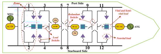
Figure 1.
MVDC shipboard power system architecture.
2.1.1. Generation Model
SPS power generation system, such as MTG or ATG, has two components, gas turbine and synchronous generator.
According to the characteristics of the gas turbine and the fuel power curve, the dynamic model of the gas turbine can be approximated as shown in Equation (1). The dynamic model of gas turbine has a output and a control inputs . presents the power transferred to the power turbine load, which is . denotes the normalized control input. and can obtain through specific fuel consumption curves and surface plots of power equations for engine [33].
The dynamic model of synchronous generator is given as follws. This dynamic model has one output and two control inputs and . In the physical sense, and are the same.
The output power of generators has to be constrained to keep the safe operation and avoid mechanical damage. Those inequality constraints are described as follows: denotes the power ramp rate of generation system.
2.1.2. Propulsion Module
This part is composed of a propulsion motor which provides the power output . The output power of the generation part is taken as one of the control inputs of the model , and the desired power is output by adjusting the normalized command power .
The operational constraints for this part are as follows:
2.1.3. Power Network Model
In this paper, the total output power of the power generation system is meet the demand power of all loads in normal operation and three kinds of loads are considered: vital loads, semi-vital loads, and non-vital loads. Vital loads are always required for normal condition, which cannot be short of electricity. Semi-vital loads can be interrupted in a short-time when emergencies occur, while the non-vital loads can be actively shed to maintain the demand power of the vital and semi-vital loads. Vital and semi-vital loads can be supplied by the PB or SB side bus using redundant switches, as shown in Figure 1, the non-vital loads directly connect to port side or starboard side bus. It is assumed that, loads can be controlled by a load shedding switch. In this paper, load shedding is only considered for non-vital loads.
To improve the reliability of power delivery for zonal loads, a redundant switch design is used in zonal SPS. As shown in Figure 1, in zone i, every vital and semi-vital loads can only be powered by PB side or SB side bus at a certain time, which is determined by the redundant switches and . If and , the power for vital and semi-vital loads in zone i are delivered by PB side bus. Thus, the power network model and constraints in zone i are can be described as Equation (6).
is the total demand power in zone i at time t, is the state of redundant switches. , and are the electric power demand of vital, semi-vital loads and non-vital loads, respectively. , and are weighting factors of three kinds of loads. The value of weighting fator are associated to prioritize service for different types of load. In this paper, , and are set for analysis.
2.2. Problem Formulation
The control objectives of this paper are to restore the normal operation of ship power grid from the fault state and to achieve the following performance attributes:
- (1)
- optimizing the switch configuration to maximize the supplied power for loads.
- (2)
- maintaining power quality of the SPS and minimizing bus voltage deviation.
The system studied in this paper has discrete variables such as switching transformation and continuous variables, which is a typical hybrid system. Therefore, the control objectives can be transformed into a hybrid model predictive control (HMPC) problem. Thus, using the backward Euler method, the dynamic model can be transfered into mixed logic dynamic (MLD) model, which is represented in the following equations:
where
In the above equations, , and are the MTG electric power demand, ATG electric power demand as well as the propulsion system power demand as the continuous control inputs. is the DC bus voltage. and are total electric power of propulsion load and service loads, respectively. denotes the sample time interval. The parameters , , are the constants used in the MLD, which is similar in [29].
Taking the switches states as the discrete control input and introducing the logic variable , and , Equation (8) is transformed into the following expresses. denotes the state of redundant switches connect to the PB or SB.
Substituting Equation (9) into Equation (7), we can get the standard MLD state space equation of SPS dynamic model, as shown below.
where
Here, A, C, , , , are coefficient matrices of corresponding terms. is the state variable, is the control variable, and is the binary auxiliary variable. is the constraint function corresponding to the control inputs and is the constraint function of state variables, these forms of constraints are used in the next section.
Considering the control objectives and operational constraints, the HMPC problem can be established as follows:
where
and
for all , subject to Equations (3), (5), (6) and (9).
Here, is the desired DC bus voltage, , , present weighting factors of different terms in the objective function. The first term in , the deviation between the desired bus voltage and the measured system bus voltage, reflects the control objective of bus voltage tracking. Minimizing this term can maintain power quality on SPS. The second term is designed for maximizing the loads demand electric power delivered. The Φ(N) is the terminal cost function to penalize the error of the bus voltage and power from the desired value using weighting factors of and , respectively.
The control objective of SPS failure recovery determines that to solve the nonlinear HMPC problem Equation (12) with constraints, an efficient optimization algorithm is needed to meet the rapidity requirements.
3. Problem Solution and Analysis
The problem in Equation (12) is transformed into a MINLP problem, and then the nonlinear branch and bound (NLP-BB) method is used to complete optimization, and the open access solver CPLEX is called. However, the computation speed is slow because the problem contains discrete variables and nonlinear characteristics. When the intelligent optimization algorithm PSO is used to deal with the HMPC problem, the computing time value rises with the increase in the prediction horzion.
To improve the calculation speed and reduce the complexity of the calculation, this paper uses the hierarchical hybrid MPC (Hi-HMPC) algorithm to ensure the consistency of the solution results and reduce the computing time at the same time. One iteration of the proposed method is introduced in Figure 2.
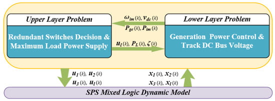
Figure 2.
Flowchart of optimal management algorithm for HMPC.
The proposed algorithm divides the solution process of the original HMPC problem into two layers of optimization problems. The upper layer is the optimization problem of redundant switch decision. Since the output power of the power generation system cannot undergo a sudden rise or drop at the moment of switch combination changes, the generation power and load consumption power can be considered as known quantities that can be obtained from the current system state. Then, the optimized switch combination is solved, and the new power network structure and load power state are obtained. The lower layer problem is the optimization of output power generation and the dynamic tracking of DC bus voltage. In this problem, the optimal combination of switches is regarded as known, and the power generation is optimized according to the power supply demand of the SPS grid to minimize the voltage deviation. After the problems of two layers are solved, a set of optimized control sequence is obtained and output into the system.
3.1. Upper Layer Solution
Due to the continuous variable that cannot be mutated is considered as known quantities, the original HMPC problem Equation (12) can be transformed into a form of nonlinear mixed-integer nonconvex programming (NMINP). However, mixed-integer programming with logical auxiliary variables and nonlinear parts, such as switch control variables, is a nonlinear and non-convex problem. As mentioned earlier, the computation is complicated. For the reduction in computational complexity, the constraints of switch control variables are relaxed and the inequality condition are transformed into any value between 0 and 1, , while the constraints of logical variables and Equation (6) remain unchanged. Then, the original problem is transformed into an approximately convex relaxed integer optimization which can be handled by a simpler solution, such as interior point-based solvers [34].
To illustrate the efficiency of the upper layer algorithm, the computational complexity is analyzed [35,36]. The CPLEX solver mentioned earlier is called to solve the original NMINP problem with branch and bound (BB) method maintaining a upper bound and a lower bound on the objective value which can be considered as a suboptimal solution of the global optimum. Here, the optimization problem is assumed as convex, and the upper and lower bound of the global optimal value are found. When the deviation between the upper and lower bounds is less than a certain constant , the solver creates branches for the switch control variables and forms subproblems. After relaxing the constraints of switches, it generates upper and lower bounds on the optimum of subproblems. Eventually, fixing a varibel with unfixed parent node to creat each leaf node, a binary tree is formed and the nodes in the tree at certain depth corresponds to the switch variables of the certain subproblems generated before. Then, the bounds of the optimal value can be get through minimizing the upper and lower bounds of each node.
The programming terminates when is satisfied the convergence requirement. Therefore, a complete binary tree with depth of n, the number of the switch control variables, has the computational complexity of . However, the proposed solution makes a complexity of for the worst case which is much less than the BB-based method, m denotes the number of constraints. Furthermore, in this stage, continuous state variables such as generation power and load power are assumed to be fixed values, which means that the original equation can be simplified as an optimization problem only related to logical variables. At this time, the non convex source of the optimization problem is only the constraints of continuous variables and logical variables, and the continuous variables do not work, so the optimization problem can be regarded as a convex optimization problem after the constraints are relaxedThe local optimal solution of convex optimization problem is the global optimal solution, so the proposed method has the same result as MINLP.
3.2. Lower Layer Solution
In this layer, the SPS grid structure, the logic variables and discrete variables in HMPC are known. In this case, the lower layer problem are considered as the optimal control problem to solve the optimal control sequence in the future finite prediction horizon.
For the HMPC problem in Equation (13), using the minimum principle (MP), Lagrange operators , and are introduced to construct Hamiltonian function, then the original formula is transformed into the following express.
and assuming the problem has an optimal solution, the following equations should be satisfied.
where and are the constraints for state variables and control variables mentioned in Equation (10). Since there is constraints of the control variable, which means , it is necessary to discuss the analytical solution of in order to solve the above equation, which increases the computational complexity.
To avoid this problem, the idea of perturbation analysis (PA) is applied here. Due to the characteristics of continuous variables in SPS, it can be considered that the continuous state variables of the system do not change much from the current sampling interval to the next. Assuming that the initial steady-state value and are the optimal sequence, the optimal solution at can be approximated by the optimal solution and the perturbed optimal sequence , .
The original problem of solving the optimal solution at is transformed into the problem of solving , which is about the optimal control problem of . To obtain the optimization solution of the developed problem, the variational method is applied to . The equation is given in Equation (17).
where
It is assumed that the problem has an optimal solution, using the minimum principle, Lagrange operators are introduced and Hamiltonian equation is constructed again, then the new function satisfies the following conditions.
When solving the upper layer problem, the generation power remains unchanged, which means that the non-vital loads will be shed by the optimization algorithm when the power is insufficient. Therefore, the perturbation caused by and will not make and violate the constraint. At this point, can be considered as unconstrained. Then the following equations is true.
4. Simulation Results
In this section, the real-time simulation results of the proposed optimization algorithm under two scenarios are given. The solutions to the switch combination optimization problem are compared wtih MINLP and PSO algorithm. The voltage fluctuation of DC bus, output power of MTG and ATG and total demand power of loads are shown to illustrate the dynamic control performance of the propsoed method. The real-time simulator in Figure 3 is used to verify the effectiveness and real-time feasibility of the algorithm. In order to reveal the efficiency of the algorithms, computation time efficiency (CTE) is introduced, which is defined as follow.
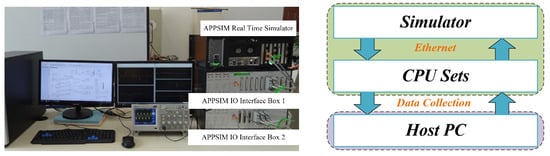
Figure 3.
Real time simulator and system configuration.
The SPS grid structure considered in this section is shown in Figure 4 and the switch combination under normal operating condition is given in Table 2 where 1 means close and 0 means break off. Four DC load zones and two propulsion loads are delivered power by the main generation system and auxiliary generation. Under normal operation, the output power of MTG and ATG are 8 MW and 4 MW, respectively. The DC load zones have the three kinds of loads mentioned before while the propulsion loads are treat as vital loads. The electric power of each propulsion load is 1 MW while the other loads are serviced full power operating condition. The parameters used for the rest of this study is given in Table 3, the prediction horizon is 5, the control horizon is 1 and is set as 1 ms.
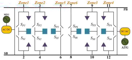
Figure 4.
Schematic view of SPS under pre-fault state.
Table 2.
Switch configuration (pre-fault).
Table 3.
Simulation parameters.
4.1. Scenario 1
In this part, a scenario where faults occur between branches 3–5, 8–10 and 9–11 is considered. The branches of PB between 3 and 11 are left without power fed by MTG or ATG and the switches of load zones in this portion need to change to maintain the power supply of the loads though the SB based on their priorities. As shown in Figure 5 and Table 4, the optimal reconfiguration opens , and closes , to ensure maximum power supply to the vital and semi-vital loads. The nonvital loads attaced to PB at node 9 and node 11 are shed because of the power generation limitation of ATG while the other loads are normally serviced. The total electric power demand drops to 11 MW and the ATG has to operate in the full capacity condition. As seen from Table 4, the proposed algorithm and the other two solver produce the same switch combanation in this fault scenario.
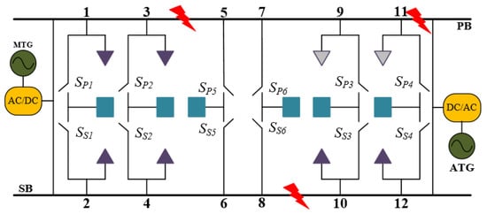
Figure 5.
Schematic view of SPS under fault scenario 1.
Table 4.
Switch configuration in fault scenario 1.
The dynamic control effect of scenario 1 in the whole fault recovery process which cannot be shown in the studies where the assumption of a smooth transition of system state is present in Figure 6. When the system runs stably for 0.5 s, scenario 1 occurs. To recover the power grid from the failure, the proposed algorithm is applied. During the operation of the method, due to the branch fault between 3–5, 8–10 and 9–11, the load of the system decreases and the voltage rises instantaneously which can be seen in Figure 6. The power generation system begins to adjust the output power to maintain the bus voltage stability. After switch reconfiguration, the maximum load of the system is restored to 11 MW. Under the regulation of control algorithm, the output power of MTG is adjusted to 7 MW, the output power of ATG is stabilized at 4 MW, and the voltage gradually returns to the expected value.
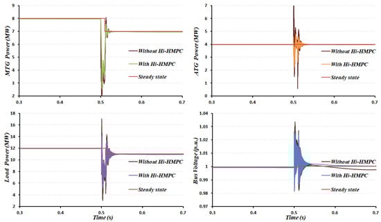
Figure 6.
Performance demonstration of Hi-HMPC in real time simulation of scenario 1.
4.2. Scenario 2
Here, two faults occur between branch 1–3 and 10–12 when the propulsion system accelerates in this scenario. Starting from the initial state, the propulsion system speeds up, while the propulsion load power demand gradually increases. At 7 s, two faults occur at the position as shown in Figure 7. Before the failure, the output power of MTG increased to 11.5 MW, while ATG was still in full load operation and all loads were normally powered. In order to maximize the load supply and minimize the bus voltage fluctuation, the proposed optimization algorithm provides the optimal switch reconfiguration, which requires the closing of , and opening and . After switch reconfiguration, the electric power of loads in zone 4, nonvital loads connected to PB side bus at node 3 and node 9 are supplied by ATG, and the rest are powered by MTG. The switch status compilation in this scenario can be seen in Table 5.
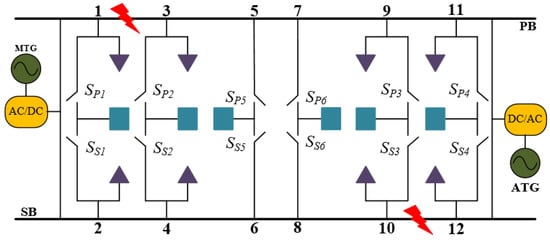
Figure 7.
Schematic view of SPS under fault scenario 2.
Table 5.
Switch configuration in fault scenario 2.
As the propulsion load demand power continues to rise, according to the priority of loads, one of the nonvital loads attached to the bus on PB side and SB side at nodes 1, 2, 4 and 10 has to be shed due to the power generation limitation of MTG. Here, we assume that the nonvital load at node 1 is shed. After active shedding, the load power required by MTG is still 11.5 MW, and continues to increase with the increase in propulsion power demand. As can be seen in Figure 8, assuming the smooth transition of the system state, the dynamic change does not appear in time because only the start and end power requirements are displayed.
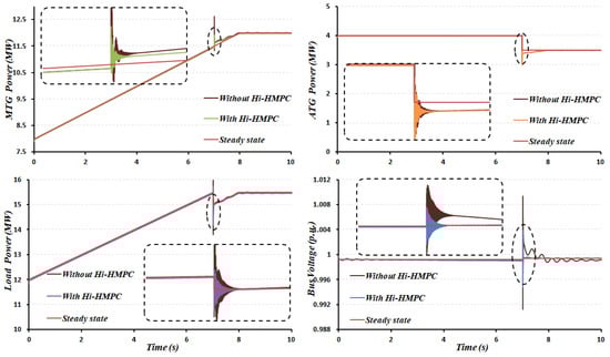
Figure 8.
Performance demonstration of Hi-HMPC in real time simulation of scenario 1.
5. Conclusions
A failure mode management control strategy for SPS optimal energy management has been proposed, analysed and verified on the real-time simulator in this study. The optimization management problem is established as a hybrid MPC problem, and carried out using Hi-HMPC algorithm. The computation efficiency of this reconfiguration strategy is enhanced through the reduction in the search space complexity, which is ensure the ability for real-time implement. The simulation results indicate the optimum for the proposed algorithm obtain the same global optimum as original MINLP formulation and PSO algorithm. The simulation results also show that the proposed method can provide a better performance in the real-time dynamics of the system, restore the power balance of the system in time, and meet the dynamic performance requirements of the system. In the future, more complex fault scenarios can be further studied, such as using the SPS model which is closer to the actual physical system, and the algorithm applying to the actual physical system for real-time testing.
Author Contributions
B.W.; methodology, B.W.; software, B.W. and P.S.; validation, L.Z. and B.W.; investigation, X.P. and B.W.; resources, L.Z. and P.S.; data curation, P.S. and B.W.; writing—original draft preparation, B.W.; writing—review and editing, X.P. and B.W.; project administration, L.Z. and X.P.; funding acquisition, L.Z. and X.P. All authors have readand agreed to the published version of the manuscript.
Funding
This research was funded by the Ministry of Industry and Information Technology of People’s Republic of China (25B0-02) and supported by the Fundamental Research Funds for the Central Universities (3072020CFT2403).
Institutional Review Board Statement
Not applicable.
Informed Consent Statement
Not applicable.
Data Availability Statement
Not applicable.
Conflicts of Interest
The authors declare no conflict of interest.
References
- Doerry, N.; McCoy, K. Next Generation Integrated Power System: NGIPS Technology Development Roadmap; Naval Sea Systems Command: Washington, DC, USA, 2007. [Google Scholar]
- Doerry, N. Naval Power Systems. IEEE Electrif. 2015, 3, 12–21. [Google Scholar] [CrossRef]
- Hebner, R.E.; Uriarte, F.M.; Kwasinski, A.; Gattozzi, A.L.; Estes, H.B.; Anwar, A.; Mccoy, T.J. Technical cross-fertilization between terrestrial microgrids and ship power systems. J. Mod. Power Syst. Clean Energy 2016, 4, 161–179. [Google Scholar] [CrossRef]
- Ahuja, A.; Das, S.; Pahwa, A. An AIS-ACO hybrid approach for multi-objective distribution system reconfiguration. IEEE Trans. Power Syst. 2007, 22, 1101–1111. [Google Scholar] [CrossRef]
- Ramos, E.R.; Martinez-Ramos, J.L.; Exposito, A.G.; Salado, A.J.U. Optimal reconfiguration of distribution networks for power loss reduction. In Proceedings of the 2001 IEEE Porto Power Tech Proceedings, Porto, Portugal, 10–13 September 2001; Volume 3, p. 5. [Google Scholar]
- Guimaraes, A.N.; Lorenzeti, J.F.C.; Castro, C.A. Reconfiguration of distribution systems for stability margin enhancement using tabu search. In Proceedings of the 2004 International Conference on Power System Technology, 2004. PowerCon 2004, Singapore, 21–24 November 2004; Volume 2, pp. 1556–1561. [Google Scholar]
- Panasetsky, D.; Sidorov, D.; Li, Y.; Ouyang, L.; Xiong, J.; He, L. Centralized emergency control for multi-terminal VSC-based shipboard power systems. Int. J. Electr. Power Energy Syst. 2019, 104, 205–214. [Google Scholar] [CrossRef]
- Jin, X.; Zhao, J.; Sun, Y.; Li, K.; Zhang, B. Distribution network reconfiguration for load balancing using binary particle swarm optimization. In Proceedings of the 2004 International Conference on Power System Technology, 2004. PowerCon 2004, Singapore, 21–24 November 2004; pp. 507–510. [Google Scholar]
- Srivastava, S.K.; Butler-Purry, K.L. Probability-based predictive self-healing reconfiguration for shipboard power systems. IET Gener. Transmiss. Distrib. 2007, 1, 405–413. [Google Scholar] [CrossRef]
- Seenumani, G.; Peng, H.; Sun, J. A reference governor-based hierarchical control for failure mode power management of hybrid power systems for all-electric ships. J. Power Sources 2011, 196, 1599–1607. [Google Scholar] [CrossRef]
- Bose, S.; Pal, S.; Natarajan, B.; Scoglio, C.M.; Das, S.; Schulz, N.N. Analysis of optimal reconfiguration of shipboard power systems. IEEE Trans. Power Syst. 2012, 27, 189–197. [Google Scholar] [CrossRef]
- Nelson, M.; Jordan, P.E. Automatic reconfiguration of a ship’s power system using graph theory principles. IEEE Trans. Ind. Appl. 2015, 51, 2651–2656. [Google Scholar] [CrossRef]
- Amba, T.; Butler-Purry, K.L.; Falahi, M. Genetic algorithm-based damage control for shipboard power systems. In Proceedings of the 2009 IEEE Electric Ship Technologies Symposium, Baltimore, MD, USA, 20–22 April 2009; pp. 242–252. [Google Scholar]
- Jiang, Y.; Jiang, J.; Zhang, Y. A novel fuzzy multiobjective model using adaptive genetic algorithm based on cloud theory for service restoration of shipboard power systems. IEEE Trans. Power Syst. 2012, 27, 612–620. [Google Scholar] [CrossRef]
- Kanellos, F.; Anvari-Moghaddam, A.; Guerrero, J. A cost-effective and emission-aware power management system for ships with integrated full electric propulsion. Electr. Power Syst. Res. 2017, 150, 63–75. [Google Scholar] [CrossRef]
- Haung, Y. Fast Reconfiguration Algorithm Development for Shipboard Power Systems. Master’s Thesis, Mississippi State University, Starkville, MS, USA, 2006. [Google Scholar]
- Kumar, N.; Srivastava, A.; Schulz, N.N. Shipboard power system restoration using binary particle swarm optimization. In Proceedings of the 2007 39th North American Power Symposium, Las Cruces, NM, USA, 30 September–2 October 2007; pp. 164–169. [Google Scholar]
- Padamati, K.R.; Schulz, N.N.; Srivastava, A.K. Application of genetic algorithm for reconfiguration of shipboard power system. In Proceedings of the 2007 39th North American Power Symposium, Las Cruces, NM, USA, 30 September–2 October 2007; pp. 159–163. [Google Scholar]
- Qudaih, Y.; Hiyama, T. Reconfiguration of power distribution system using multi agent and hierarchical-based load following operation with energy capacitor system. In Proceedings of the 2007 International Power Engineering Conference, Singapore, 3–6 December 2007; pp. 223–227. [Google Scholar]
- Feng, X.; Butler-Purry, K.L.; Zourntos, T. A multi-agent system framework for real-time electric load management in MVAC all-electric ship power systems. IEEE Trans. Power Syst. 2015, 30, 1327–1336. [Google Scholar] [CrossRef]
- Das, S.; Bose, S.; Pal, S.; Schulz, N.N.; Scoglio, C.M.; Natarajan, B. Dynamic reconfiguration of shipboard power systems using reinforcement learning. IEEE Trans. Power Syst. 2013, 28, 669–676. [Google Scholar] [CrossRef]
- Xu, Q.; Yang, B.; Han, Q.; Yuan, Y.; Chen, C.; Guan, X. Optimal Power Management for Failure Mode of MVDC Microgrids in All-Electric Ships. IEEE Trans. Power Syst. 2019, 34, 1054–1067. [Google Scholar] [CrossRef]
- Mitra, P.; Venayagamoorthy, G.K. Real-time implementation of an intelligent algorithm for electric ship power system reconfiguration. In Proceedings of the 2009 IEEE Electric Ship Technologies Symposium, Baltimore, MD, USA, 20–22 April 2009; pp. 219–226. [Google Scholar]
- Mitra, P.; Venayagamoorthy, G.K. Implementation of an intelligent reconfiguration algorithm for an electric ship’s power system. IEEE Trans. Ind. Appl. 2011, 47, 2292–2300. [Google Scholar] [CrossRef]
- Shariatzadeh, F.; Vellaithurai, C.B.; Biswas, S.S.; Zamora, R.; Srivastava, A.K. Real-time implementation of intelligent reconfiguration algorithm for microgrid. IEEE Trans. Sustain. Energy 2014, 5, 598–607. [Google Scholar] [CrossRef]
- Zohrabi, N.; Abdelwahed, S.; Jian, S. Reconfiguration of MVDC shipboard power systems: A model predictive control approach. In Proceedings of the 2017 IEEE Electric Ship Technologies Symposium, Arlington, VA, USA, 15–17 August 2017. [Google Scholar]
- Kekatos, N.; Forets, M.; Frehse, G. Modeling the Wind Turbine Benchmark with PWA Hybrid Automata. In Proceedings of the 4th International Workshop on Applied Verification of Continuous and Hybrid Systems, Pittsburgh, PA, USA, 18–20 April 2017; Volume 48, pp. 100–113. [Google Scholar]
- Khakimova, A.; Kusatayeva, A.; Shamshimova, A.; Sharipova, D.; Bemporad, A.; Familiant, Y.; Rubagotti, M. Optimal energy management of a small-size building via hybrid model predictive control. Energy Build. 2017, 140, 1–8. [Google Scholar] [CrossRef]
- Sarailoo, M.; Rezaie, B.; Rahmani, Z. MLD Model of Boiler-Turbine System Based on PWA Linearization Approach. Int. J. Control. Sci. Eng. 2012, 2, 88–92. [Google Scholar] [CrossRef]
- Du, J.J.; Song, C.Y.; Li, P. Multilinear model control of Hammerstein-like systems based on an included angle dividing method and the MLD-MPC strategy. Ind. Eng. Chem. Res. 2009, 48, 3934–3943. [Google Scholar] [CrossRef]
- IEEE Recommended Practice for 1 kV to 35 kV Medium-Voltage DC Power Systems on Ships; IEEE Std, 1709-2010; IEEE: New York, NY, USA, 2010; pp. 1–54.
- IEEE Recommended Practice for Electrical Installations on Shipboard-Design; IEEE Std, 45.1-2017; IEEE: New York, NY, USA, 2017; pp. 1–198.
- Doktorcik, C.J. Modeling and Simulation of a Hybrid Ship Power System. Master’s Thesis, Department Electrical Computer Engineering, Purdue University, West Lafayette, IN, USA, 2010. [Google Scholar]
- Yurii, N.; Nemirovskii, A. Interior Point Polynomial Time Methods in Convex Programming; SIAM: Philadelphia, PA, USA, 2004. [Google Scholar]
- Grossmann, I.E. Mixed-integer nonlinear programming techniques for the synthesis of engineering systems. Chem. Res. Eng. Des. 1990, 1, 205–228. [Google Scholar] [CrossRef]
- Floudas, C.A. Nonlinear and Mixed-Integer Optimization: Fundamentals and Applications; Oxford University Press: London, UK, 1995. [Google Scholar]
Publisher’s Note: MDPI stays neutral with regard to jurisdictional claims in published maps and institutional affiliations. |
© 2021 by the authors. Licensee MDPI, Basel, Switzerland. This article is an open access article distributed under the terms and conditions of the Creative Commons Attribution (CC BY) license (https://creativecommons.org/licenses/by/4.0/).