A Progressive Period Optimal Power Flow for Systems with High Penetration of Variable Renewable Energy Sources ^†

Abstract

Renewable energy sources including wind farms and solar sites, have been rapidly integrated within power systems for economic and environmental reasons. Unfortunately, many renewable energy sources suffer from variability and uncertainty, which may jeopardize security and stability of the power system. To face this challenge, it is necessary to develop new methods to manage increasing supply-side uncertainty within operational strategies. In modern power system operations, the optimal power flow (OPF) is essential to all stages of the system operational horizon; underlying both day-ahead scheduling and real-time dispatch decisions. The dispatch levels determined are then implemented for the duration of the dispatch interval, with the expectation that frequency response and balancing reserves are sufficient to manage intra-interval deviations. To achieve more accurate generation schedules and better reliability with increasing renewable resources, the OPF must be solved faster and with better accuracy within continuous time intervals, in both day-ahead scheduling and real-time dispatch. To this end, we formulate a multi-period dispatch framework, that is, progressive period optimal power flow (PPOPF), which builds on an interval optimal power flow (IOPF), which leverages median and endpoints on the interval to develop coherent coordinations between day-ahead and real-time period optimal power flow (POPF). Simulation case studies on a practical PEGASE 13,659-bus transmission system in Europe have demonstrated implementation of the proposed PPOPF within multi-stage power system operations, resulting in zero dispatch error and violation compared with traditional OPF.

1. Introduction

Variable renewable energy sources (VREs) including wind farms and solar sites, are increasingly integrated into power systems for environmental and climate benefits. Unfortunately, these resources exhibit characteristics of uncertainty and variability that present challenges to real-time power balancing and as a result, jeopardize the security, stability, and reliability of the power system. Without an effective solution to this challenge, VREs may be relegated to a low capacity factor, with large installed capacity and relatively low power output.

There are three main ways to reduce the downside impact of VREs from the power balancing perspective: (i) prediction techniques, which aim to increase the wind and solar forecasting accuracy [1,2]; (ii) multi-stage dispatch operations, which is focus on adjusting the refinement of traditional dispatch operations from the power balancing perspective [3,4]; (iii) balancing reserves, which utilizes conventional power sources, storage facilities, active loads, and other controllable resources to balance the supply uncertainty [5,6]. From the power balancing perspective, the dispatch hierarchy in systems is typically comprised of day-ahead scheduling, real-time dispatch, and automatic generation control (AGC). Day-ahead scheduling balances the day-ahead load forecasts while real-time dispatch manages the residual real-time power imbalance.

In more detail, day-ahead scheduling arranges base generation and reserve from controllable power sources to accommodate the potential power uncertainties from VREs during the real-time dispatch. This process also arranges the frequency modulation reserves for real-time and AGC, to ensure sufficient flexibility to achieve the overall power balance. During real-time dispatch, balancing reserve is used to manage the smaller real-time power imbalance.

During the day-ahead stage, balancing reserves are normally arranged through statistical and historical data. If balancing reserves are sufficient, fluctuations in net load can be accommodated locally. As VRE penetrations increase, it becomes even more important for adequate balancing reserves to be available locally, since reliance on import/export may become less desirable. In the absence of available downward reserves, some renewable power will be spilled or delivered to the neighboring system, and the equivalent transmission line capacity connected with the neighboring system should be reduced accordingly to deliver the VREs outside.

2. Literature Review

The optimal power flow (OPF), proposed by J. Carpentier in 1962 [7], is a fundamental building block of the above decisions, implemented into multiple time periods over successive intervals in the overall dispatch hierarchy [8,9,10]. In this section we review the OPF and its various refinements to set the stage for the proposed framework to coordinate optimal dispatch decisions across the multi-stage dispatch process.

The power system decision processes currently use the OPF to incorporate uncertainty of VRE sources by developing dispatch and reserve schedules based on forecasts for these VREs. While the power system is operated on a continuous basis, these forecasts are provided at discrete intervals, effectively providing a discretized dispatch schedule [11,12]. Output levels between these discrete points are approximated by linear interpolation, so that the forecasted output becomes a piece-wise linear function of time [13,14].

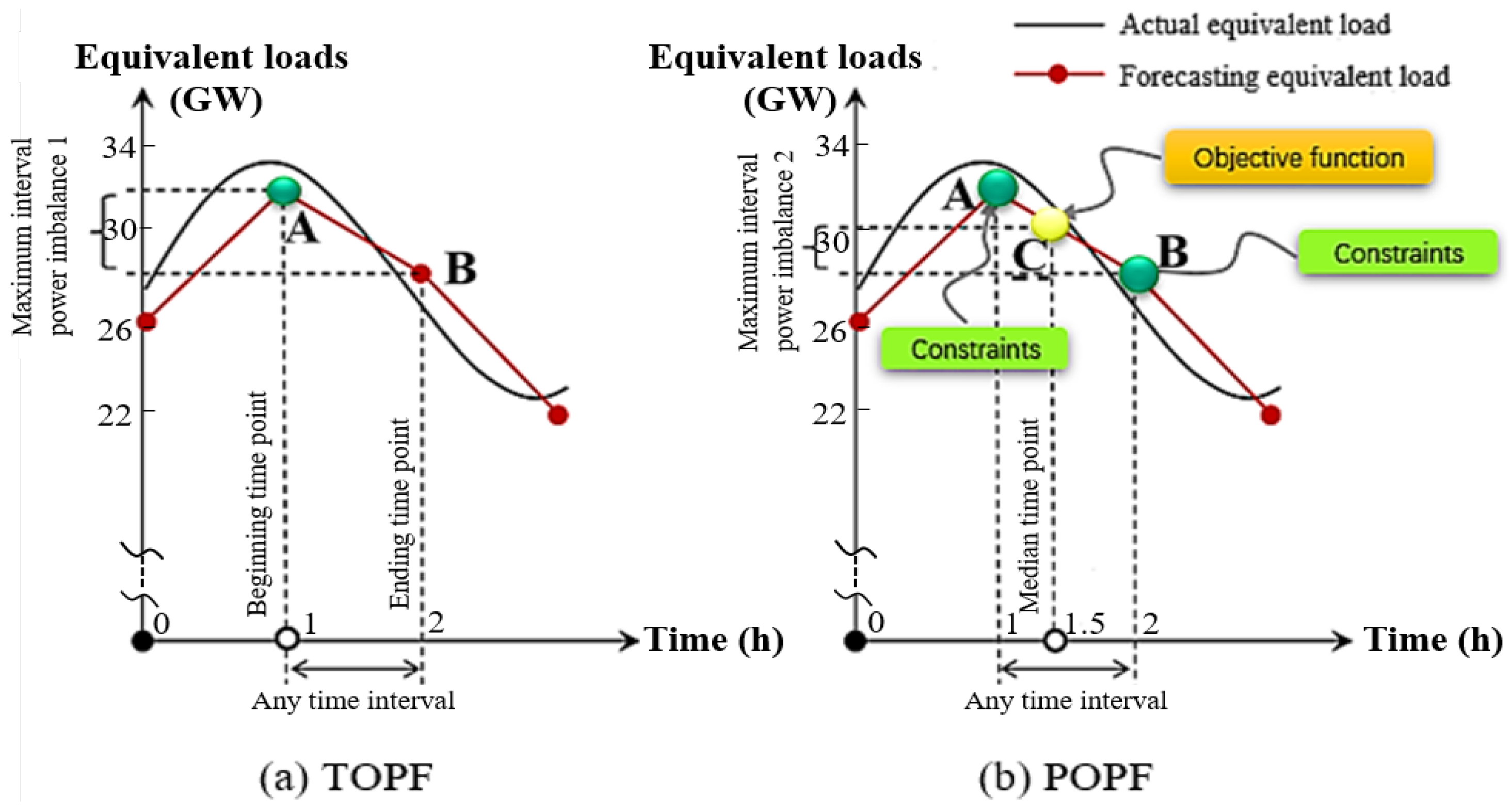
During both day-ahead and real-time scheduling, the OPF problem is solved sequentially for future discrete points in time, resulting in a stepwise optimal generation schedule that periodically adjusts the controllable power outputs [12,15,16]. This use of a discrete time OPF for the continuous problem is visualized in Figure 1, wherein traditional optimal power flow ensures is optimal at discrete points in time (typically the initial point of a time interval, for example point A), and assumes that the solution will satisfy the operational constraints until the subsequent solution point, for example point B, which is the initial point for the next time interval 2.

In reality, the discrete points may not accurately represent the intermediary operating points, and it is not guaranteed that solutions obtained at the discrete points will satisfy all the other constraints continuously between the points. Moreover, the increasing adoption of variable and distributed resources presents operational challenges that can lead to more constraint violations within a time period. Therefore, it is necessary to come up with an efficient OPF approach that ensures the power flow balance, voltage constraints, and thermal limits to be satisfied at all time points within a given interval [17,18,19,20,21].

The rigorous OPF model for a time horizon contains a set of temporal constraints and is a large-scale, non-linear, and time-varying optimization problem which is costly to solve. Therefore, any increase in the number of computational points associated with solutions of higher temporal resolution leads to challenges in providing optimal solutions in a timely manner.

Over time, there have been various refinements developed in the literature. In [22], to cover multiple time periods, a dynamic optimal power flow (DOPF) model was proposed as an extension of TOPF. This approach is initially developed for hydrothermal power systems to dispatch subject to intertemporal technologies such as energy storage and flexible demand [23]. DOPF models have been studied and applied in the assessment of interruptible demand management [24]; dispatch of energy and ancillary services [25]; active and reactive power dispatch with embedded generation and battery storage [26]; operations of distribution networks with uncertainties from distributed generators [20]; and dispatch strategy for microgrids with storage [27]. Compared with TOPF, DOPF aims to provide an optimal solution over a time period to ensure continuity in system performance; however, the replication of constraints for each time point across the horizon significantly complicates the computation. As a result, this approach is less advantageous due to its time-consuming nature.

An alternative approach is the decomposition of time steps over a time period, as proposed in [20]. There are also several examples of multi-period OPF (MOPF) models, which seek to develop a staged solution across a time horizon. For example, Matpower’s optimal scheduling tool (MOST) was developed in [28] to solve generalized steady-state electric power scheduling problems including a deterministic single period economic dispatch problem, stochastic security-constrained unit-commitment and multi-period OPF problem [29]. A flexible and advanced OPF approach based on MOST was presented in [30], where the authors adopted the DC approximation and highlighted the dynamic computational challenge of simultaneously handling multiple periods. In [31], the authors proposed a MOPF to solve scheduling and OPF problems over a finite horizon with Benders decomposition. Subsequently, ref. [32] proposed a linearized AC-MOPF model in low voltage systems to solve optimal problem for an infinite control horizon. Regardless of the intervention, the computational burden of any MOPF grows with the number of time steps making problems of practical size intractable.

This computational burden can be addressed through judicious linearization. In non-linear dynamic problems, an important approach is to partition the entire time period into several smaller continuous time intervals. These sub-intervals must be selected to balance the computational burden with accurate representation of the continuous problem. This trade-off is explored through optimal selection of discrete time steps in [21]. From the perspective of economic efficiency, a continuous-time economic dispatch model for a specific time interval was proposed in [33], which linearized system frequency and generator dynamic constraints on sub-minute intervals. However, the voltage constraints were not considered in [33] and the captured points that interconnect intervals were not clearly explained. In [21], a characteristic optimal power flow (COPF) model was analyzed to optimize power system performance over a single time period, which simplifies the DOPF and improves efficiency over the TOPF. This was explored in a simulation framework with linearized AC power injections over a time period.

Extending to multiple time periods, the work described in [34] proposed the concept of a linear-time interval (LI), in which the active and reactive power injections can be represented by linear mappings of time. As previously discussed, the concept of a LI is already implied in operational models, as a result of the discrete time intervals in multi-stage power system dispatch operations. For example, in day-ahead scheduling, forecasts are predicted hourly and as a result, one hour LIs are implied over the 24 h timescale. In intra-day or real-time operations, the dispatch interval varies depending on market rules and levels of VREs in the system, ranging from 15 min to one hour [11,35,36]. As a result of this framework, the nodal voltages can also be shown to be approximately linear in time, over the same interval [34]. However, it may be possible to improve the accuracy of the dispatch decisions across the planning horizon by incorporating constraints at additional time intervals without a significant increase in computational burden, by leveraging the linearity of these intervals.

To ease the computational burden and to more effectively characterize the continuous time period in models like [21,34], a consecutive linearization technique of the OPF is proposed in this paper. In this framework proposed here, a given time period is partitioned into multiple consecutive LIs, and the OPF within each LI is defined as interval optimal power flow (IOPF). Under the LI assumption, there is an approximate linear relationship between system states (e.g., nodal active and reactive power injections, nodal voltages) and time. To increase accuracy across the interval, the IOPF model includes the median time point and two terminal time points of the interval, as shown in Figure 2b. Specifically, the IOPF minimizes the objective function at the median time point (C) while enforcing operational constraints from two terminal points (A and B), as shown in Figure 2b. The efficacy of this strategy is based on the following: (i) with voltage as an approximate linear function of time, the monotonicity of a LI ensures that constraints are satisfied at any internal point of the LI as long as the constraints are satisfied at the two terminal points, and (ii) previous work in ([34], Figures 8 and 14) shows that the median time point and two terminal time points hold the smallest interval voltage error. An OPF model over a time period is then derived by consecutive IOPFs, where the terminal solution for a time period becomes the initial solution for the next period. Since the proposed OPF model takes into consideration the entire time period, it is then referred to as the period optimal power flow (POPF) model. The success of POPF model is demonstrated through application in day-ahead scheduling and real-time dispatch, respectively. A progressive period optimal power flow framework (PPOPF) that coordinates the day-ahead POPF and real-time POPF is proposed and integrated into an overall dispatch hierarchy. An example of coherent coordinations among IOPF, day-ahead POPF, real-time POPF, and PPOPF is given in Figure 3.

The remainder of this paper is organized as follows. A comprehensive methodology framework is devised in Section 3, in which each of the layers, or the sub-components of the PPOPF framework in Figure 3 are describe. The IOPF, day-ahead POPF and real-time POPF methodologies are analyzed to show a coherent coodination of integration of these layers together in the framework. Validation and simulation results of the proposed methodologies on a PEGASE 13,659-bus system are carried out in Section 4 and conclusions are finally given in Section 5.

3. Methodology and Framework

This section develops the model and algorithm of the proposed progressive optimization in the multi-stage dispatch framework. The develop of the IOPF and its algorithm is first described, as well as the coordination of IOPFs between adjacent intervals. The formulation of the PPOPF if then described, to illustrate the coordination of the IOPFs across multiple consecutive intervals, considering both the day-ahead and real-time operations.

3.1. Interval Optimal Power Flow

The lowest level of the framework partitions a time period into several smaller intervals which can be represented as linear-time intervals (LIs). According to the mean-value theorem, the IOPF optimizes the objective function at the median time point to characterize the average economic efficiency over the time interval. Note that such a representation is rigorous as long as the linear assumption holds. Based on the defined LI, IOPF simplifies the continuous optimization of each interval into a three-time-point IOPF as follows:

Since the nodal complex voltage is approximate linear with respect to time, the two extreme load conditions in a LI are guaranteed to exist at two terminal time points. If the inequality constraints are satisfied on the terminal time points, then they are also satisfied at any other point within the LI. According to the grid frequency modulation property, the IOPF checks the branch power and voltage limits on two terminal time points.

In this way, the IOPF linearizes and discretizes the continuous OPF over sub-intervals into a three-time point OPF, significantly simplifing the overall model as follows:

(1) Median time point based objective function: For any linear-time interval, the objective function is evaluated at the median time point, it could be either cost or profit, such as minimizing market cost, generation cost, or transmission losses. In addition, since energy can be directly priced and traded, the objective function is directly related to energy. So the median timepoint, has the energy integral property. Generally, the median-time point based objective function can be expressed as:

$$\forall T_k:minf(U,X,t_k^m),$$

(1)

where U is a set of control variables, X is a set of state variables, and $t_k^m$ is the median time point.

(2) Constraints for median time point: For any linear-time interval $T_k$, since the inequality constraints are satisfied at within the interval as long as these constraints are satisfied at two terminal time points. Therefore the power flow equality constraints are considered into the median time point:

$$\forall T_k:h(U,X,t_k^m)=0.$$

(2)

(3) Constraints for two terminal time points: For any linear-time interval $T_k$, the equality and inequality constraints must be satisfied at both terminal time points $t_{k-1}$ and $t_k$. The power flow equality constraints are

$$\forall T_k:\left\{\begin{array}{c}h(U,X,t_{k-1}^{})=0\hfill \\ h(U,X,t_k^{})=0\hfill \end{array}\right..$$

(3)

The nodal complex voltage inequality constraints are

$$\forall T_k:\left\{\begin{array}{c}{V}_{min}\le V\left(t_{k-1}\right)\le V_{max}\hfill \\ V_{min}\le V\left(t_k\right)\le V_{max}\hfill \end{array}\right.,$$

(4)

the lower bound and upper bound are usually considered as 0.95 p.u. and 1.05 p.u., respectively. The controllable power inequality constraints are

$$\forall T_k:\left\{\begin{array}{c}{P}_{min}^c\le P_{}^c\left(t_{k-1}\right)\le P_{max}^c\hfill \\ Q_{min}^c\le Q_{}^c\left(t_{k-1}\right)\le Q_{max}^c\hfill \\ P_{min}^c\le P_{}^c\left(t_k\right)\le P_{max}^c\hfill \\ Q_{min}^c\le Q_{}^c\left(t_k\right)\le Q_{max}^c\hfill \end{array}\right.,$$

(5)

and the line power inequality constraints are

$$\forall T_k:\left\{\begin{array}{c}{P}^{line}\left(t_{k-1}\right)\le P_{max}^{line}\hfill \\ P^{line}\left(t_k\right)\le P_{max}^{line}\hfill \end{array}\right..$$

(6)

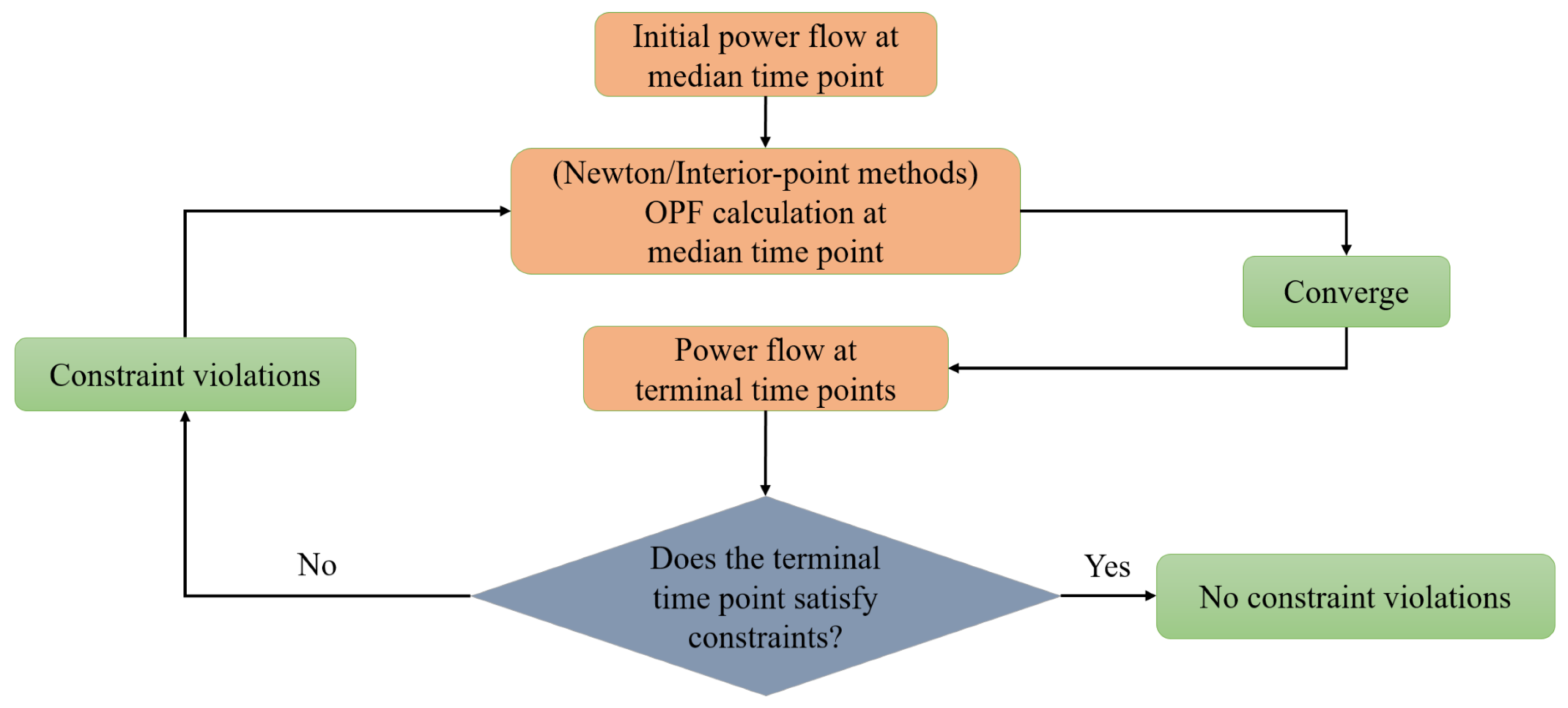
Specifically the IOPF algorithm is based on an objective function at the median time point, where the corresponding controllable power sources are adjusted in ways of either linear peak regulation or frequency modulation. From this, the power flow constraints at the two bounding time points on the interval are calculated and enforced. If there are no constraint violations then the IOPF calculation is terminated. Otherwise, the controllable power limits are adjusted based on the nodal voltage constraint violations, and a median time point based OPF is recalculated iteratively until all constraints are satisfied. If adjustments are no longer successful in satisfying the constraints at the terminal time points, for example, if the solution does not converge within a tolerance level (e.g., ${10}^{-6}$), then the solution which most closely satisfies the terminal condition is adopted as the optimal solution.

The IOPF algorithm is shown visual in Figure 4, and consists of two parts: median time based optimization, with constraints applied at the terminal time points.

As loading conditions are similar in between adjacent linear-time intervals, the solution from the previous linear-time interval is taken as the initial value for the next linear-time interval:

$$\left\{\begin{array}{c}{P}_0^c\left(t_k^m\right)=P^c\left(t_{k-1}^m\right)\hfill \\ V_0^c\left(t_k^m\right)=V^c\left(t_{k-1}^m\right)\hfill \end{array}\right.,(k=1,2,...,N),$$

(7)

where $P_0^c$ and $V_0^c$ respectively represent the initial values of active power and nodal voltage magnitude for controllable sources; N is the total number of terminal time points.

According to the proposed LI, the combined nodal voltage time-varying function, and the corresponding numerical simulation case studies [34], under any LI, power flow calculations at three specified time points (median and two terminal time points), are the most accurate solutions. Combined with IOPF, the power flow and constraint violations are enforced accordingly, for a computationally efficient and accurate solution.

The IOPF methodology needs to be applied over the multi-stage dispatch process; with multiple time periods and (sub-) time periods, considering the entire horizon requires coordination between day-ahead and real-time POPFs including: connection between adjacent intervals; coherence of balancing reserve and utilization; and progressive optimizations between day-ahead scheduling and real-time dispatch. In this formulation, the computational efficiency arising from linearity enables the integrated solution of day-ahead scheduling and real-time dispatch in a PPOPF framework, described in Section 3.2.

3.2. Progressive Period Optimal Power Flow

The first component of the PPOPF is coordinating the LIs between day ahead and real time.

3.2.1. Coherent Connection between Day-Ahead and Real-Time

As previously described, the PPOPF includes relevant dispatch timescales and their corresponding LIs into sequential IOPFs. The POPFs are then constructed by consecutive IOPFs.

For day-ahead scheduling, the timescale is 24 h with the LI typically chosen as 1 h, which is a typical forecasting interval at this stage. Thus the timescale is divided into 24 LIs in which each LI is solved by IOPF to obtain optimal objective value while satisfying sets of constraints over the LI. The day-ahead POPF algorithm is constructed by connecting all IOPFs from different LIs.

Similarly, it is important to determine appropriate timescale from the power balancing perspective for real-time dispatch. Existing literature acknowledges the importance of timescale design in the power balancing architecture and offers suggestions on possible timescales such as 4 h, 2 h, and 1 h [11,16,35,36,37]. However, neither systematic studies nor theoretical analysis nor analytical formulations have been characterized or constructed to design the timescale for real-time dispatch, despite the potential consequences. If the selected timescale for real-time dispatch is too long, then there may not be sufficient conventional resources or frequency modulation reserves to balance the manage power imbalance in real-time. Conversely, if the real-time dispatch timescale is too short, unnecessary computational burden will result.

Sufficient conventional resources to accommodate the uncertainty levels of VREs and appropriate timescale designs with theoretical analysis are the fundamentals for the real-time dispatch to achieve the best possible power balancing function through the whole power systems. Therefore, a proper timescale that appropriately represents the tradeoff between the forecasting accuracy and the computational efficiency is highly desirable. From the power balancing perspective, paper [12] described the theoretical functions, power balancing architecture, and the hierarchical design of the dispatch control systems with different high penetrations of VREs. More specifically, it proposed an analytical formula to achieve appropriate real-time dispatch timescale given different power systems with different high penetration of VRE integration. In addition, paper [12] also theoretically clarified the relationship between the balancing reserve capacities of day-ahead scheduling and real-time dispatch power balancing function, as well as the relationship between AGC power adjustment capabilities and power forecasting accuracy of real-time dispatch.

Detailed connections among real-time dispatch timescale, day-ahead scheduling timescale, and the LIs between them are shown in Figure 5. The red curve is day-ahead forecasts over the 24 h timescale and the corresponding LI is 1 h. The blue curve is the real-time dispatch which is a rolling-forward window period with the timescale is 1 h and the corresponding LI is 15 mins. To better incorporate the day-ahead scheduling timescale, the LIs and their respective timescales should have integer relations as shown in Figure 5. Similar with day-ahead scheduling, each LI under real-time dispatch timescale is solved by IOPF. Thus the real-time POPF algorithm is further constructed.

Compared with real-time dispatch, the timescale for day-ahead scheduling (24 h) and its LI (1 h) are longer, resulting in larger forecast error and a more approximate result. Since the timescale for real time dispatch and its LI are smaller, the forecast accuracy is expected to be significantly improved. Real-time POPF uses this more accurate information to update and correct the more approximate day-ahead POPF to better represent conditions and help system’s power balancing process.

3.2.2. Balancing Reserve Utilization between Day-Ahead and Real-Time

Before presenting the day-ahead and real-time POPF algorithms, since the balancing reserve utilization including local reserve delivery principles described in the Introduction section has coherent correlations between day-ahead and real-time POPFs, it is necessary to first analytically characterize a few issues, for example, how to arrange the amount of balancing reserves according to the day-ahead VRE forecasting uncertainty; what are the conditions that need to be satisfied accordingly if the local balancing reserve does not have the capability to fully balance the real-time power imbalance; how to deploy the balancing reserves from neighboring systems, etc. To answer issues like these, this subsection characterizes the local balancing reserve delivery between day-ahead and real-time. Note that, this part will be helpful in understanding how the balancing reserves are dispatched and utilized later in the simulation section with a practical power system.

Ref. [38] has designed a statistical quantification towards the VRE uncertainty in power systems. Therein, a negative-exponential forecast uncertainty function $\alpha$ is constructed to describe the relation between the statistics of VRE forecasting error and time-ahead, in which the amplitude A represents the VRE day-ahead uncertainty and satisfies the relation in (8). Due to page limits, more details about $\alpha$ function can be found in [38].

$$\mathrm{A}\propto \frac{P-P_s}{P_s},$$

(8)

where $P,P_s$ are the total actual power and total day-ahead forecast power, respectively. We get

$$\Delta P=P-P_s,$$

(9)

where $\Delta P$ represents power imbalance of day-ahead generation schedules. Therefore,

$$\mathrm{A}\propto \frac{\Delta P}{P_s}.$$

(10)

Since

$$\Delta P=P-P_r+P_r-P_s,$$

(11)

considering real-time forecast $P_r$ is much closer to actual power, $P-P_r\approx 0$, the real-time power imbalance $\Delta P_r$ can be then approximated as

$$\Delta P_r=P_r-P_s\approx \Delta P.$$

(12)

According to (8), the proportion of balancing reserve with day-ahead forecast is given by

$$\Delta P_r\propto \mathrm{A}{P}_s,$$

(13)

and can be switched to the following equation from recent real-time power imbalance data

$$P_R=\rho \mathrm{A}{P}_s,$$

(14)

where $P_R$ is balancing reserve, $\rho$ is the adjustment coefficient.

A larger $\rho$ helps to better accommodate power imbalance during real-time POPF, resulting in an increased spinning reserve from controllable power sources. Therefore, the adjustment coefficient $\rho$ needs to be appropriately selected.

The goal of optimal dispatch in power systems with high penetration of VRE is to obtain the maximum penetration of VRE, which is supported by coherent coordination between day-ahead POPF and real-time POPF, which are derived by consecutive IOPFs within different numbers of LIs (in different timescales). If the balancing reserves from local sources and neighboring systems are $\Delta P_n$ and $\Delta P_0$, the upper bound for outside power delivery in day-ahead generation schedules is then reduced to:

$${\tilde{P}}_L=P_L-\Delta P_o.$$

(15)

Since

$$\Delta P=\Delta P_n+\Delta P_o,$$

(16)

we get

$${\tilde{P}}_L=P_L-\Delta P+\Delta P_n.$$

(17)

According to (15)–(17), it is evident to see that, if there is enough local balancing reserve to accommodate the VRE uncertainties, then $\Delta P_o=0$, and the power capacity limit for neighboring power snapshot remains the same, ${\tilde{P}}_L=P_L$.

Local balancing also provides coordination between day-ahead scheduling and real-time dispatch. The day-ahead POPF arranges balancing reserve, and real-time POPF utilizes the balancing reserve, which are both based on local balancing.

The first step while making real-time generation schedules is to forecast the net loads, after which the real time power imbalance $\Delta P_r$ is identified. If local balancing reserve has the capability to fully balance the real-time power imbalance, then real-time POPF is calculated within the local balancing reserve capacity. Otherwise, the balancing reserve is first set as upper bound value before running the real-time POPF.

3.2.3. Day-Ahead POPF

The tasks in day-ahead scheduling regarding power balance are as follows: (i) develop day-ahead generation schedules based on day-ahead load forecasts; in other words, make base load and peak regulation schedules; (ii) arrange balancing and frequency modulation reserve. More details are presented with the corresponding day-ahead POPF diagram in Figure 6.

(1) Forecast day-ahead equivalent loads.

(2) According to day-ahead forecast results, local balancing reserve is achieved in (14). Prepare the frequency modulation based on power system regulations.

(3) Check the local balancing reserve capacity. If the local balancing reserve is enough to balance the power imbalance from the real-time dispatch, then arrange the order from different types of accommodation sources. Otherwise, update and correct the upper bound for power neighboring delivery in (17).

(4) For controllable power sources aside from balancing reserve, day-ahead POPF gives the minimum generation cost. The constraint violations on two endpoints are enforced by peak regulation in each LI. Nuclear power units are included in the base load schedule process with constant values and thus are not involved in balancing.

According to Figure 6, day-ahead POPF is shown as follows.

For any LI, let $P_M$ be local controllable power sources, if

$$P_M\ge P_R,$$

(18)

then the amount of local balancing reserve is arranged as $P_R$. The remaining part $\Delta P_M$, that is,

$$\Delta P_M=P_M-P_R,$$

(19)

participates in the day-ahead generation scheduling plan. Thus the optimization set for POPF is

$$P_s^c=\Delta P_M+P_g^{out},$$

(20)

where $P_s^c$ is power generation from control variables U; $P_g^{out}$ is controllable power sources from neighboring systems.

If

$$P_M<P_R,$$

(21)

then the local controllable power sources are allocated as balancing reserve, with the corresponding optimization set

$$P_s^c=P_g^{out}.$$

(22)

The remaining reserves

$$\Delta P_0=P_R-P_M,$$

(23)

are supplied from neighboring systems. The upper bound for power outside delivery is then corrected and updated as

$${\tilde{P}}_L=P_L-\Delta P_o.$$

(24)

The above optimization set $P_s^c$ and the corrected upper bound value ${\tilde{P}}_L$ are substituted into IOPF model. Hence the day-ahead POPF in power systems with high penetrations of VREs under local balancing reserve is thus developed.

3.2.4. Real-Time POPF

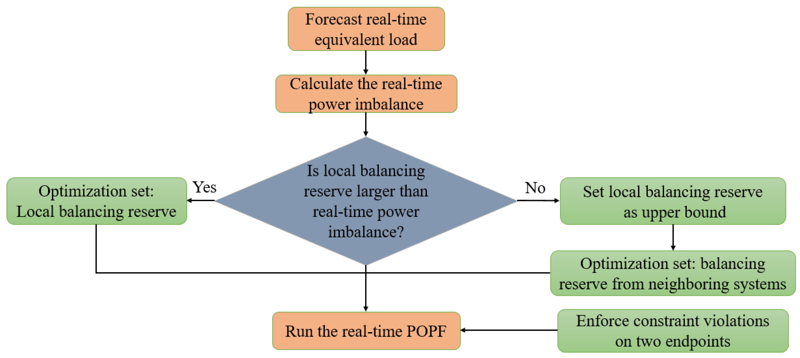
From the power balance perspective, real-time dispatch is mainly focused on accommodating the VRE uncertainties and is a coordinated update to the day-ahead scheduling decisions. The detailed steps for making real-time generation schedules are presented as follows with the corresponding real-time POPF diagram shown in Figure 7.

(1) Update forecasts for the real-time equivalent loads.

(2) According to real-time forecast results, balancing reserve is obtained in (12).

(3) If the local balancing reserve capacity is larger than the real-time power imbalance, then the optimization set is restricted within local balancing reserve capacity given by

$$P_r^c=\Delta P_M.$$

(25)

Otherwise, the local balancing reserve is set as upper bound, and the optimization set is the balancing reserve from neighboring systems, that is,

$$P_r^c=P_g^{out},$$

(26)

where $P_r^c$ is power generation from control variables U; $P_g^{out}$ is controllable power sources from neighboring systems. By substituting $P_r^c$ into the IOPF model, a real-time POPF model in power systems with high penetration of VRE under local balancing is developed.

(4) Run real-time POPF with optimization set. During each LI, constraint violations on two endpoints are enforced by real-time peak regulation and AGC frequency modulation.

4. Results

For power systems with high penetrations of VREs, the use of these sources is contingent on sufficient capacity of controllable assets that provide peak regulation, frequency modulation, balancing reserve and/or security reserve in the systems. Achieving maximum penetrations of VREs requires coordination with controllable assets, in other words, power systems without controllable assets are not currently feasible.

Since controllable assets necessarily exist in power systems, objective functions between minimum generation cost of conventional assets and maximum penetration of VRE are not contradictory while considering the deep peak regulation without the cost. Thus, the objective function in this paper is to minimize controllable power generation cost. Based on this objective, the performance of the PPOPF framework is considered on a case study using the relatively large PEGASE test system, which is described in more details below.

4.1. PEGASE 13,659-Bus System

A PEGASE 13,659-bus system is further tested in this paper to illustrate the effectiveness of proposed PPOPF. This system accurately represents the size and complexity of the European high voltage transmission network which contains 13,659 buses, 4092 generators, and 20,467 branches [39]. Since some parts of the system are aggregated, some generators (e.g., with negative PMIN) represent aggregations of multiple negative loads and generators, modifications are given in this case studies, where 2315 wind generators and 1157 solar generators are added, a more detailed case system with network topology, can be found https://matpower.org/docs/ref/matpower6.0/case13659pegase.html, accessed on 16 Decenber 2016. Some values are given as follows:

(1) Controllable power capacity is 417,518 MW.

(2) The maximum wind and solar forecasts in all the 24 day-ahead LIs are 67,185 MW and 16,796 MW, respectively. The corresponding load forecast is 361,717 MW. Therefore, the equivalent load forecast is 277,735 MW.

(3) Without loss of generality, total power generation is equal to total loads. Thus the total generation with the highest wind power output forecast is 361,717 MW, wind power generation is 80% of VREs and VRE generation is 20% of the total capacity.

(4) Day-ahead uncertainty of total power generation A is 19%.

4.2. Simulation Studies on Day-Ahead POPF

The steps of day-ahead POPF are shown as follows.

(1) Balancing reserve

Balancing reserve is arranged in (14) according to equivalent load forecasts, wherein $P_e^s$ = 277,735 MW, A = 19%. To fully accommodate VRE, the adjustment coefficient $\rho$ is selected as 1.1. The balancing reserve is 75,599 MW.

(2) Check local balancing reserve capability

Controllable assets dispatched from day-ahead generation schedules do not include the balancing reserve prepared for real-time dispatch, which is 341,919 MW. Since local controllable assets (341,919 MW) are larger than the maximum day-ahead wind power forecasts (83,981 MW), the VRE uncertainty can be accommodated through local balancing reserve and it is not necessary to be delivered from neighboring balancing reserves. Therefore, controllable assets dispatched from day-ahead generation schedules are 341,919 MW.

(3) Day-ahead generation scheduling plans

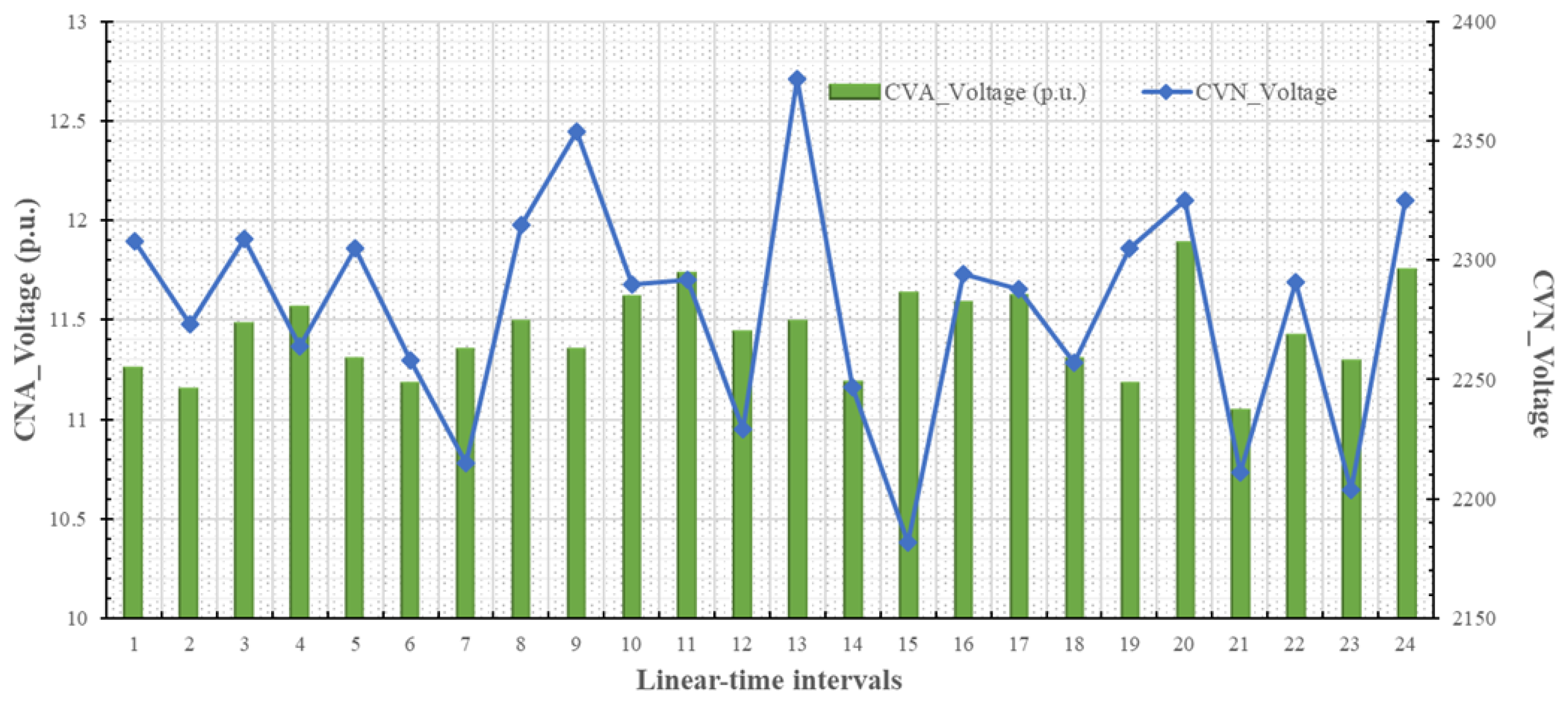
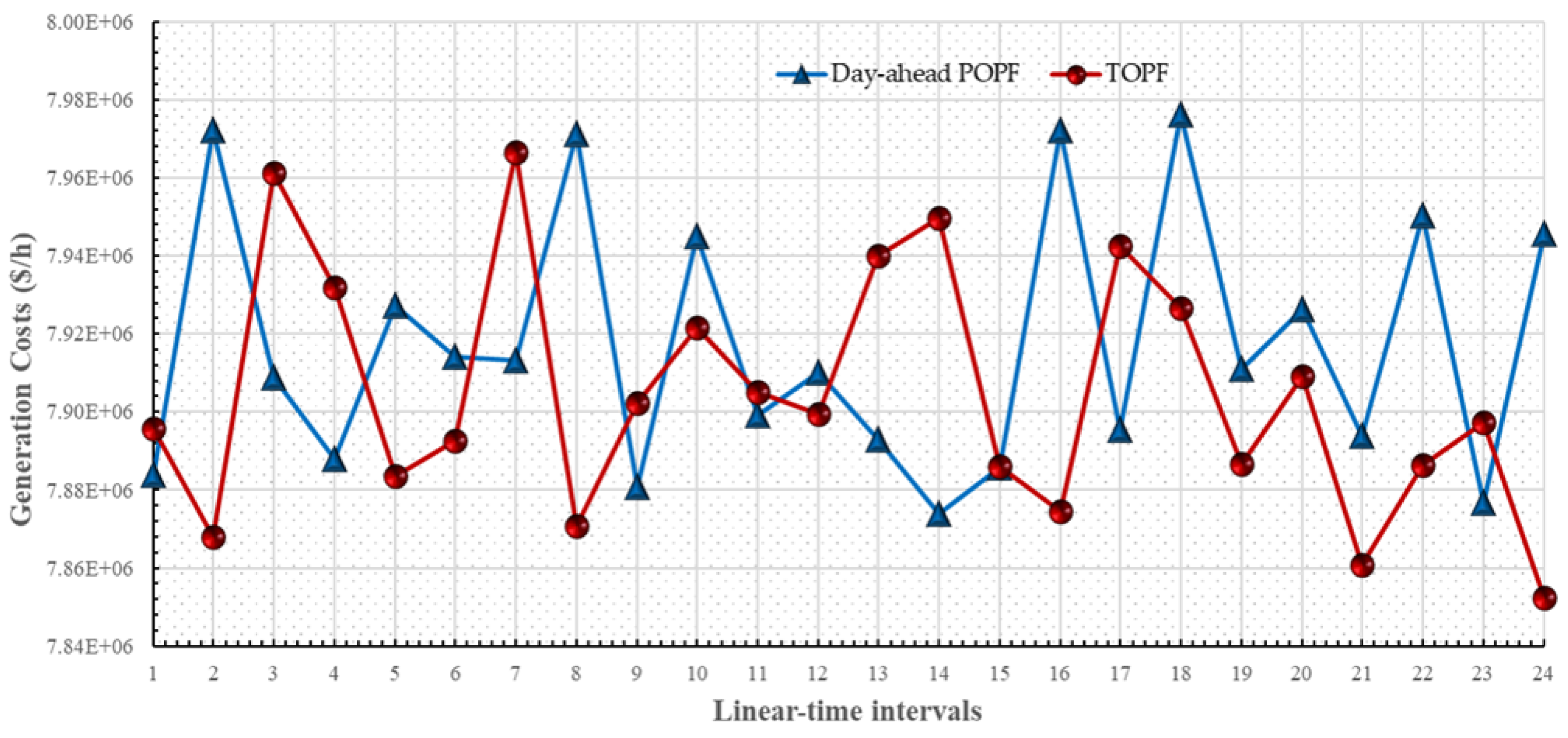
Since the timescale of day-ahead scheduling is 24 h, we divide the 24 h into 24 LIs. According to the day-ahead load forecasts, the day-ahead POPF are run with a minimum generation costs of controllable power sources (exclude balancing reserve). Under each LI, the constraints violations are checked on two endpoints through peak regulation. Meanwhile, a TOPF model is applied and constraint violations are enforced. Comparison results between POPF and TOPF from 24 LIs are shown from Figure 8, Figure 9 and Figure 10. The optimization output of day-ahead POPF enables a later progressive real-time dispatch.

All the operational constraints for the 24 LIs are satisfied in the day-ahead POPF. The TOPF, on the contrary, produces over-limits for branch power and voltage magnitude violations, as shown in Figure 8 and Figure 9. wherein the “CVN” and “CVA” represent constraint violation numbers and constraint violation amounts. Therefore, unlike the day-ahead POPF, the TOPF results in both thermal and voltage constraint violations in all the 24 LIs.

Generation costs between two models are compared in Figure 10, where generation costs of day-ahead POPF are still close to but generally larger than TOPF. Likewise, generation costs of day-ahead POPF is smaller than TOPF on certain LIs, such as the 4 th LI, since the TOPF optimizes on the initial time point while the total loads monotonically decrease over the interval, thus resulting in over-generation. However, in other cases, equivalent loads have different trends, either upward or downward, leading to constraint violations when decisions are made on the initial time point only.

4.3. Simulation Studies on Real-Time POPF

From a power balance perspective, real-time dispatch accommodates VRE uncertainties and is focused on real-time power balance. The combination of controllable power generation after PPOPF must be satisfied by the available capacity of controllable assets.

Under real-time dispatch, the optimization set is local controllable assets if there is adequate balancing reserve. Otherwise, the local controllable assets are set as upper bound and the remains will be dispatched from neighboring systems.

The same system from PEGASE 13,659-bus system is tested and analyzed in this section. The first step for real-time POPF is to design a proper timescale for real-time dispatch from the power balancing perspective. In this case study, according to (17)–(19) in [12], we select the timescale is 1 h.

Note that since the real-time dispatch timescale is a rolling window, the initial time is selected to correspond to the beginning of the one-hour LI for day-ahead scheduling, in which the corresponding day-ahead forecasting loads are applied to achieve the real-time power imbalance. We then divide the 1h into 4 LIs, indicating each LI is 15 min.

We next check to see if local balancing reserve is adequate enough to accommodate VRE uncertainty. Since the maximum real-time forecast is 157,542 MW, real-time power imbalance is 73,562 MW according to (12). Due to the local balancing reserve (75,599 MW), which is larger than real-time power imbalance, it is thus selected as the optimization set.

Based on the coherent connections between real-time dispatch and day-ahead scheduling, TOPF and real-time POPF are both applied into real-time dispatch. Power generation costs and constraint violations are thus obtained, respectively, with the corresponding results shown in

Table 1. Comparisons Between traditional optimal power flow and Real-time period optimal power flow.

LI	Parameters	TOPF	Real-Time POPF
0 h–0.25 h	CVN-Power	884	0
	CVA-Power (MW)	1939	0
	CVN-Voltage	457	0
	CVA-Voltage (p.u.)	3.2093	0
	Generation cost ($/h)	9.01 × 10${}^6$	8.92 × 10${}^6$
0.25 h–0.5 h	CVN-Power	940	0
	CVA-Power (MW)	2235	0
	CVN-Voltage	529	0
	CVA-Voltage (p.u.)	3.0347	0
	Generation cost ($/h)	$8.91\times {10}^6$	$8.84\times {10}^6$
0.5 h–0.75 h	CVN-Power	921	0
	CVA-Power (MW)	2348	0
	CVN-Voltage	491	0
	CVA-Voltage (p.u.)	3.1029	0
	Generation cost ($/h)	$8.98\times {10}^6$	$8.87\times {10}^6$
0.75 h–1 h	CVN-Power	851	0
	CVA-Power (MW)	2176	0
	CVN-Voltage	563	0
	CVA-Voltage (p.u.)	3.1147	0
	Generation cost ($/h)	$8.99\times {10}^6$	$8.91\times {10}^6$

.

As shown in Table 1, real-time POPF satisfies all constraints in all the 4 LIs. The TOPF, on the contrary, results in thermal limit violations in the overall 4 LIs and a number of voltage constraint violations, though objective values of real-time POPF and TOPF are very similar.

Another interesting observation is that both the objective function values of TOPF and POPF from real-time dispatch are larger than TOPF and POPF from day-ahead scheduling. Day-ahead scheduling optimizes the deterministic net loads, wherein the generation costs include base load costs and peak regulation costs. Nonetheless, real-time dispatch optimizes deterministic net loads and non-deterministic uncertainty, wherein generation costs include base load costs, peak regulation costs, as well as balancing reserve scheduling costs. As a result, generation costs from real-time dispatch are generally larger than day-ahead scheduling.

5. Conclusions

Traditional optimal power flow (TOPF) describes system performances only on a single time point while applying the resulting decisions to an entire time period. Interval optimal power flow (IOPF) was first proposed on a linear-time interval (LI), in which the real and reactive power injections are linear mapping of time during multi-stage dispatch operations. The IOPF model takes median time point as objective function and two terminal points as constraints. Period optimal power flow (POPF) POPF is then constructed from consecutive IOPFs and is demonstrated within the multiple stages of the dispatch hierarchy, through day-ahead scheduling and real-time dispatch. These stages are then integrated in a coordinated scheme labeled the progressive period optimal power flow (PPOPF). Results explore the performance of the PPOPF framework in power systems with high penetration of variable renewable energy sources (VREs). To this end, more VREs are possible to be utilized and dispatched in the proposed PPOPF framework under guaranteeing systems’ security and stability. This paper is summarized as follows:

Three characteristics of day-ahead and real-time POPFs are evaluated in this paper: exploring connections in different LIs, the relations between balancing reserve and utilization, and progressive optimizations between day-ahead scheduling and real-time dispatch. A PPOPF model is proposed to provide these characteristics in an overarching framework.

In addition to this, to better utilize high penetration of VREs, sufficient quantity of balancing reserve is critical. A local balancing reserve to accommodate the uncertainties is described to reduce VRE fluctuations and uncertainty. Based on the local balancing, the power limit for outside delivery in day-ahead POPF, and the optimization range of controllable power in real-time POPF are then determined.

Simulation case studies on a PEGASE 13,659-bus system have validated the efficacy of the proposed IOPF, POPF and PPOPF models in fully dispatching and accommodating VRE uncertainties, eliminating dispatch error and violations that arise from the traditional OPF under the same conditions.