Article

Machine Learning-Based Classification of Electrical Low Voltage Cable Degradation

by
Egnonnumi Lorraine Codjo
1,2,*,
Bashir Bakhshideh Zad
2,*,
Jean-François Toubeau
2,*,
Bruno François
1 and
François Vallée
2
1
Centrale Lille, Arts Et Metiers Institute of Technology, University of Lille, JUNIA, ULR 2697-L2EP, F-59000 Lille, France
2
Power Systems & Markets Research Group, Electrical Power Engineering Unit, University of Mons, B-7000 Mons, Belgium
*
Authors to whom correspondence should be addressed.
Energies 2021, 14(10), 2852; https://doi.org/10.3390/en14102852
Submission received: 31 March 2021 / Revised: 30 April 2021 / Accepted: 11 May 2021 / Published: 15 May 2021

Abstract

:
Low voltage distribution networks have not been traditionally designed to accommodate the large-scale integration of decentralized photovoltaic (PV) generations. The bidirectional power flows in existing networks resulting from the load demand and PV generation changes as well as the influence of ambient temperature led to voltage variations and increased the leakage current through the cable insulation. In this paper, a machine learning-based framework is implemented for the identification of cable degradation by using data from deployed smart meter (SM) measurements. Nodal voltage variations are supposed to be related to cable conditions (reduction of cable insulation thickness due to insulation wear) and to client net demand changes. Various machine learning techniques are applied for classification of nodal voltages according to the cable insulation conditions. Once trained according to the comprehensive generated datasets, the implemented techniques can classify new network operating points into a healthy or degraded cable condition with high accuracy in their predictions. The simulation results reveal that logistic regression and decision tree algorithms lead to a better prediction (with a 97.9% and 99.9% accuracy, respectively) result than the k-nearest neighbors (which reach only 76.7%). The proposed framework offers promising perspectives for the early identification of LV cable conditions by using SM measurements.

1. Introduction

Electrical low voltage (LV) distribution networks are the last stage of the electrical power network, which supply many dispersed small-scale loads. A set of equipment such as MV-LV (medium voltage-low voltage) transformer substations, overhead/underground lines, protection systems, etc., compose those networks. The radial topology is widely used in LV distribution networks, with a voltage level around 230V. LV feeders are designed to feed a limited amount of end users in order to reduce the influence of an interruption. Consequently, either LV level interruption problems or LV equipment physical state problems (such as the cable ageing and deterioration) have received less attention.
The French standard NF C 15–100 (harmonized with the European standard HD 384) specifies that the insulating material of LV electrical cables must oppose the current all along the conductor [1]. In fact, the deteriorations of the insulation material can increase the discharge of leakage currents, which can create overcurrent and voltage variation issues and can decrease the efficient operation and safety of the network. In addition, LV distribution networks (initially designed for unidirectional power flows) are currently subject to the bidirectional power flows and frequent voltage variations arisen from the extensive connection of decentralized photovoltaic (PV) generations. The voltage variation problems [2,3,4] tend to increase the leakage current through the insulation material of LV cables. Monitoring the insulation material degradation then becomes a relevant issue.
Investigations have been carried out for modelling this insulation degradation through its resistivity variations. Additionally, the sensitivities of the insulation material to electrical and physical phenomena (such as stress in applied voltage) are analyzed. By studying the degradation of PVC (PVC (polyvinyl chloride)) insulated high-voltage cables, the author in [5] has shown the impact of environmental conditions (phenomena such as temperature and humidity variations) on the ageing of this insulation material. In [6], the authors developed a test procedure for electrical cable insulation material. The authors in [7] have evaluated the insulation resistance characteristics of LV cable under extreme experiments (such as flame contact, over-current, and accelerated degradation). The studies in [6,7] reveal that the network external operating conditions directly affect the insulating properties of the material. They show that the insulation resistance value is doubly inversely proportional to a 10 °C temperature increase. Reference [7] shows that accelerated degradation in the LV cable significantly reduces its equivalent life since it reduces the insulation resistance of the cable.
In the Netherlands, the research works [8,9,10] investigated underground LV cables with a focus on jacket damage. Researchers in [8] worked on how water ingress can progressively degrade the LV cable. To accomplish this, the experimental study was carried out based on two different plastic insulated cables (cross-linked poly-ethylene (XLPE) and PVC) artificially damaged by drilling an 8-mm hole into each cable. The cables have been tested in water exposure conditions and gradual degradation linked to partial discharges has been observed in the insulating material after any water evaporation phenomena. The different experiments showed that at a sufficient degree of degradation, breakdown can occur in the PVC cable (due to leakage currents) while the XLPE cable was still under operation. Indeed, the PVC, by decomposing, produces hydrogen chloride, which makes the water more conductive. In [9], the same researchers made a comparative study of how polymeric insulation materials affect degradation growing in LV underground cables. That study pointed out the major role of the insulating material decomposition in the cable degradation rate, regarding its chemical composition. From this aspect, PVC material has led to significant degradation, unlike polyurethane (PU) and XLPE. In Hungary, references [11,12,13] have studied the effects of distributed generation (DG) on the ageing and degradation of PVC insulation. Firstly, the work was focused on the thermal ageing of LV cables. Reference [11], by implementing a periodic thermal ageing test, has shown an inverse correlation between hardness and the conductive properties of the cable. In [13], the authors tracked the thermal aging of the PVC insulation material under various temperatures and different plasticizer contents. The results revealed the best PVC specimens for the monitoring and characterizing thermal aging in PVC insulated cables. However, these studies only focus on the physicochemical properties of the insulation material of cables.
Based on a diametrically opposed procedure, the study carried out in [14] has explored the physical degradation of the cable through the sensitivity analysis of LV network voltage variation to various degrees of cable insulation wear. In that work, the position and degree of insulation degradation of the cable are modelled as uncertain variables. Then, a Monte Carlo (MC) analysis process was used to characterize unknown variables. MC techniques have been widely used in the literature to capture the uncertain and unobservable physical quantities in distribution systems.
Scenario creation processes based on the MC technique have proven their effectiveness either for uncertainty impact assessment associated with generated and consumed powers at each nodes of the network as in [15,16], or for characterizing the low voltage distribution systems (in a sensitivity analysis context), as in [17]. Moreover, the uncertainty impacts associated to the electrical network parameters on the nodal voltages have been evaluated in [18,19]. Furthermore, reference [20] investigated whether and when alternative maintenance strategies, using historical data, would be more profitable than the currently used corrective maintenance.
In a recent research direction, machine learning (ML) techniques have been studied for fault detection in [21,22,23,24,25,26,27]. The study in [22] addresses the benefit of a machine learning framework for fault detection and classification in power systems. By analyzing the most used ML techniques (within consideration of fault types and metrics for those techniques evaluation), the authors have shown the benefits of supervised classifiers to reliably solve power system problems. In the same way, a part of the research in [23] was dedicated to the fault diagnosis in LV networks by using a deep neural networks approach. The results of this study allowed the authors to highlight the most influencing parameters in the fault assessment process, such as the fault resistance. In the context of grid monitoring, the authors in [25] set up a power line modems (PLM)-based solution for the diagnostics of distribution network cable. By implemented various ML algorithms (combined with several preprocessing methods), the proposed approach ensures the employment of the best algorithm for a given diagnostic procedure. The work has been oriented through a two-stage approach from the degradation detection to the ageing and localized degradation assessment of XLPE-insulated cable. The key point of this approach relies on access to the PML database. The authors of [27] investigated the role of ML in integrity analysis of subsea cables. From the design of a low frequency (LF) sonar system to the detection of the cable degradation stage through accelerated life cycle testing, their study provides a library of LF sonar responses depending on the cable types and conditions. Regarding voltage issues in the distribution network, the researchers in [28] have worked on a centralized voltage control framework within consideration of the uncertainties related to the network working conditions and its physical parameters (dependency between temperature variation and line resistance; internal resistance of the transformer and consideration of the shunt admittances of power lines by using a PI line model). The authors have implemented a fast decision-making method, which is cost-efficient since the deep reinforcement learning-based agent can automatically adapt its behavior under varying operating conditions.
The above ML-based studies give relevant and acceptable accuracy results with a good speed and a low calculation burden. However, they do not integrate the assessment of the electrical properties of the LV network cables associated to its growing insulation degradation. It will therefore be interesting to investigate the integration of those ML tools in the LV cable condition assessment. Hence, this paper focuses on the implementation of a machine learning-based framework in order to identify the cable lines that present an insulation degradation, considering the voltage and net demand variation profiles of the distribution network.
The novelty of this study resides in its proposed machine learning-based framework to identify the cable insulation wear, relying on nodal voltage and load demand variations. Through the extensive analysis of cable insulation thickness variations and load flow calculations, a synthetic database is built. Then, the observations in the dataset are classified using several predictors whose impacts are studied. Indeed, the proposed work is a novel approach, which lies in the use of data from already largely deployed smart meters. From an economic point of view, it is a cost-effective approach compared to the actual costly monitoring of HV transmission lines where specific meters and communication systems are used (as implemented in France). In the LV distribution system, it is very expensive to deploy sensors and dedicated information and communication technologies in the entire electrical network. To tackle this challenge, this research project aims to take advantage of available data from smart meters and leverage the ML capabilities in order to detect the soft (early-stage) degradation of cable insulation (regardless of the type of fault). Despite the existing literature related to fault detection in electrical networks, the main contribution of the current study lies in its proposed methodology, where the problem has been approached through highlighting the relationships between the operating conditions of network, its nodal voltages and thickness variation of cable insulation.
The remaining of this paper is organized as follows: Section 2 expresses the motivation and objectives of this study. Section 3 and Section 4 present the formulation of the insulation degradation problem and the way that the LV line is modelled in this work. In Section 5, the proposed methods of classification are introduced. Then, Section 6 presents the application cases, while Section 7 discusses the obtained results. Finally, in Section 8, the main conclusions are presented.

2. Motivation and Objectives

The degradation of the insulating material and its impact on the node voltages have been investigated by [14] through the electrical conductance variation of the cable insulation. A probabilistic framework has been proposed to that end by combining Monte Carlo simulations and load flow computations. Assuming that the degradation degree of the insulation material is an uncertain variable, the scenario creation procedure using Monte Carlo (MC) has been implemented for characterizing the above uncertainty. The load flow calculations finally determine the nodal voltages in the generated scenarios. The developed framework in [14] provides us with the insightful information about the statistical distribution of nodal voltage variations. Additionally, the probability of voltage variation appearance, under various degrees of insulation wear, has been analyzed.
The current paper is a step further on this direction. The objective is to detect the cable insulation degradation from the network operating point. To do so, relying on the generated database consisting of nodal voltages (associated with the load and generation profiles) as well as the cable insulation conditions, different machine learning techniques have been implemented. The latter in the training phase will learn what would be the possible nodal voltages linked to each load and generation profiles as well as the cable insulation conditions. Then, in the test phase, relying only on the nodal voltages (associated with the load and generation data), they will identify if the network working point corresponds to the normal conditions or if there is cable insulation degradation in the tested network. As the main contribution of this work, it paves the way to an effective and timely predictive maintenance of the LV distribution network avoiding the costly solutions for the distribution system operators (DSOs) as well as the customers.

3. Characterization of the Cables Insulation Degradation

Electrical cables are subject to mechanical damage, excessive heat, ageing of material, and electrical stress on a daily basis. These operating conditions cause degradation of the cable insulation material, and in extreme cases, the cable can totally or partially lose its insulation. As consequence, the insulation impedance decreases, which generates a leakage current flowing through the cable to the ground. Therefore, this impedance is composed of the ground resistance as well as the resistance of the degraded cable insulation. The remainder of this section focuses on calculating the resistance associated to the degraded insulation.
In a degraded cable, the leakage current flows radially outwards from the center towards the surface of the cable along its length. So, let us assume a cylindrical cable that has a total radius R, a length L and a conductor radius equal to r. The radius corresponding to the insulating material is equal to R-r. Then, let us consider an elementary section of that cable with a radius x and an insulation material thickness dx (infinitesimally small layer of insulation) [29]. The elementary cylindrical section (of area 2πLx) has an insulation resistance given by:
R i s o d x = ρ d x 2 π L x
where Riso-dx and ρ are, respectively, the resistance and the resistivity coefficient of the insulation material.
From Equation (1), the insulation resistance of the cable is calculated by integrating the thickness value dx over the radius of the insulating material [14]:
R i s o = ρ 2 π L r R d x x = ρ 2 π L ln R r  
The above equation gives a general formulation of an electrical cable insulation resistance. Then, by assuming that due to degradation the cable loses a part of its insulation thickness, the conductor radius r will remain constant while the cable radius R will reduce; radius variation will tend to decrease the insulation resistance value.

4. Modelling of the LV Line in Healthy and Degraded Conditions

4.1. Model of a Healthy Line

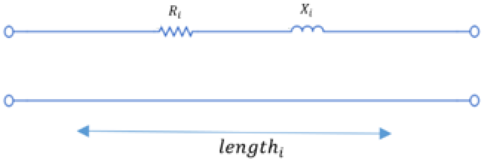
A single-phase LV line (between two nodes), in healthy condition, is modelled by its longitudinal impedance. In this study, the shunt admittances (capacitive phenomenon) from the traditional PI model are neglected because of the short distances (short cable length between system nodes; see Section 6.1) as demonstrated in [18]. Therefore, the equation of the line impedance becomes a combination of per-unit-length series resistance R i and reactance X i as:
Z i = l e n g t h i × ( R i + j X i )
where Zi is the self-impedance of the line i (between nodes i and i + 1). R i , X i and lengthi represent, respectively, the line resistance, the line reactance and the length of the line.
Figure 1 shows the series model of the above LV electrical line.

4.2. Model of a Line with Damaged Insulation

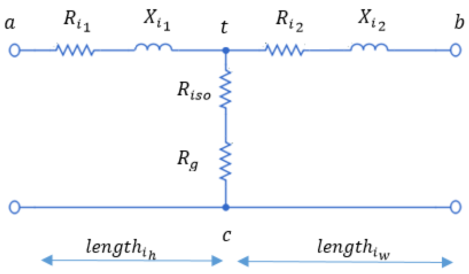
To model the electrical line, in the damaged insulation condition, the resistance variation ( R i s o ) due to the insulation degradation, established in Section 3, is incorporated in the above model, as in [14]. Indeed, a shunt variable resistance, between the leakage point (named t in Figure 2) and the ground, models the current discharge over an electrical insulation material. Figure 2 shows the representation of this new electric path (series combination of insulation resistance Riso and ground resistance Rg) in the line model.
l e n g t h i   is defined as the total length of the damaged line i while the healthy part of this line is represented by l e n g t h i h .   l e n g t h i w is the length of the section starting from the leakage point to the next node.
l e n g t h i w + l e n g t h i h = l e n g t h i
From the model in Figure 2, three impedances are defined according to the different parts of the star model [14]:
Z a t = R i 1 + j X i 1
Z b t = R i 2 + j X i 2
Z c t = R i s o + R g
To suite with the chosen load flow calculation method (presented below in Section 5.1) the «T» line model shown in Figure 2 (star connection represented by three impedances Z a t , Z b t and Z c t according to Equations (5)–(7)) is converted to an equivalent delta connection circuit represented by Figure 3.
This new PI model has resistive parallel branches with different resistance values depending on the position of the leakage point. The delta model parameters are based on the following equations:
Z A B = Z a t   Z b t + Z b t   Z c t + Z c t   Z a t   Z c t
Z B C = Z a t   Z b t + Z b t   Z c t + Z c t   Z a t   Z a t
Z A C = Z a t   Z b t + Z b t   Z c t + Z c t   Z a t   Z b t

5. Method of Analysis

5.1. Synthetic Creation of the Working Database

In the first stage, a working database is created from the cable thickness distribution and the smart meter (SM) measurements data (i.e., the load and the PV measured each quarter of an hour q). The SM inputs are used to obtain the net demand (ND).
N D i = L o a d i P V i
where NDi, PVi and Loadi are, respectively, the net demand, the PV production and the load demand at node i.
Then a load flow is computed, for each observation (each quarter q of each day), using the Newton-Raphson load flow (NRLF) technique. In this study, the NRLF technique is carried out for calculating the network nodal voltages. During NRLF computation, the nodal powers are expressed in nonlinear algebraic equations. Then, Taylor series are used to linearize those equations, which give the link between small variations in real and reactive powers as a function of small variations in the nodal voltage angles and magnitudes. The obtained Jacobian matrix is expressed as:
[ Δ P Δ Q ] = [ P θ P V Q θ Q V ] [ Δ θ Δ V ] = [ J 1 J 2 J 3 J 4 ] [ Δ θ Δ V ]
where the vectors ΔP and ΔQ represent the errors between the scheduled and calculated powers at the load buses. The vectors Δθ and ΔV represent, respectively, the variations in the nodal voltage angles and magnitudes.
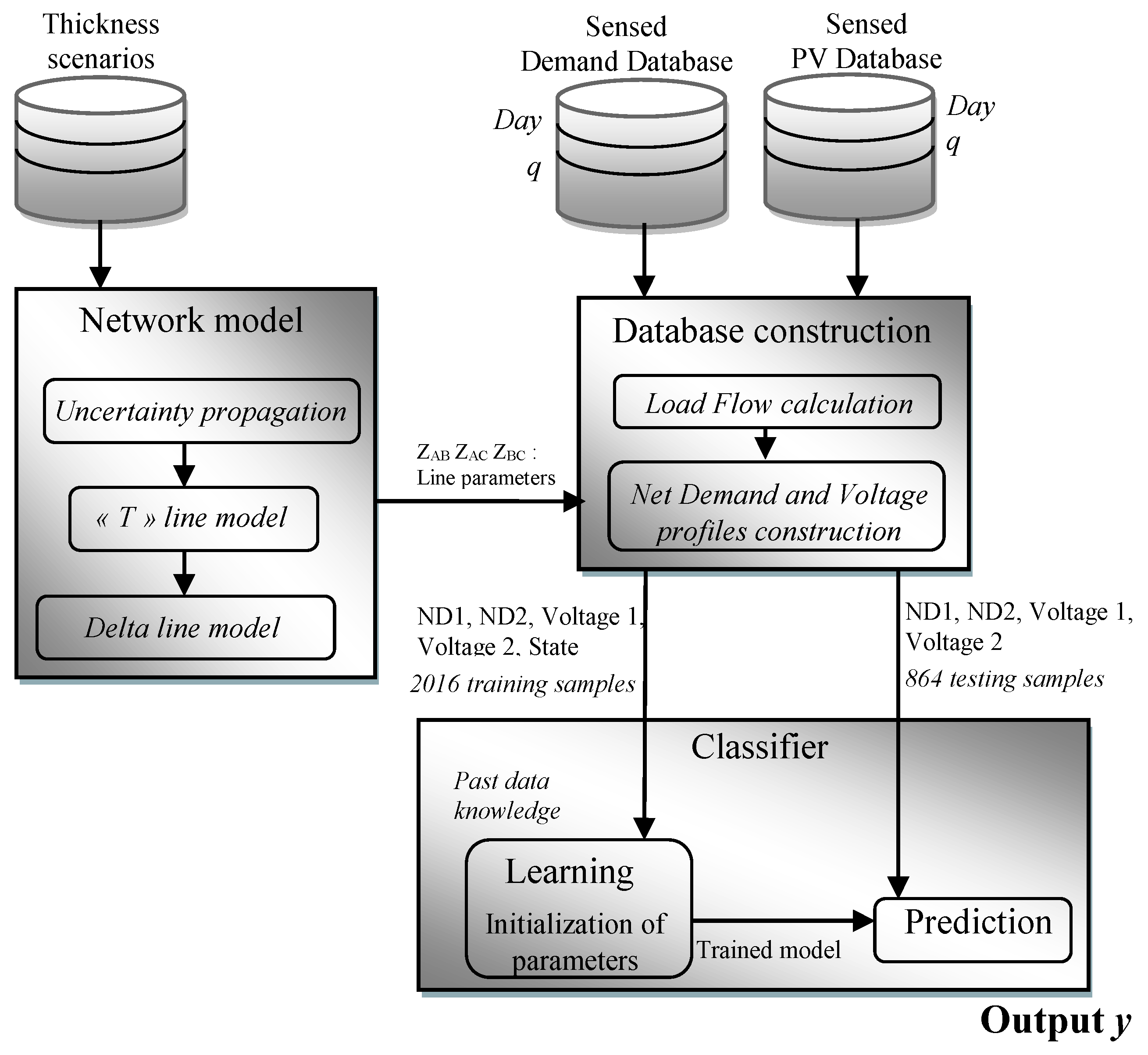
The equations for calculating the elements of the Jacobian matrix (using measured powers by the smart meter) are given in [30]. The obtained Jacobian matrix is used to update the network voltages. The ΔP and ΔQ vectors are then updated with the new voltages. For the computation of the next iteration, the Jacobian matrix elements are recalculated to obtain new network voltages, and so on, until the errors (i.e., ΔP and ΔQ vectors) are minimized to a predefined value. This is what makes the NRLF technique an iterative-based procedure. The particularity of this process is linked to the fact that the load levels are imposed for obtaining voltages of the same magnitude range as those obtained with a non-degraded cable. Figure 4 shows the flowchart of the synthetic creation of the knowledge database (the global flowchart of the proposed approach including the classification process is presented in Appendix A).

5.2. Labelling Data

For the evaluation of the cable state, two classes are defined and applied to each observation in the database (see Table 1). The class H is associated with the cables without insulation wear while the class M is used to label the cables presented a certain degree of insulation wear.

5.3. Implemented Machine Learning Methods

This subsection focuses on the machine learning (ML) aspect of the developed tool. Indeed, supervised learning approaches are ML techniques based on input and output data (labeled data) and are employed for classification. The objective is to automatically generate knowledge rules from a database containing “samples” of inputs and corresponding outputs so that with a new input data, the output variable can be predicted (as represented by Figure 5).
Regarding supervised learning approaches, they can be divided into two categories [31]:
  • Classification methods, which dispatch the input observations in categorical groups and lead to the construction of predictive models for discrete responses.
  • Regression methods, which describe the relationship between input variables (so-called predictors) and the outputs (through a mathematical function) and lead to the construction of predictive models for continuous responses.
In what follows, the supervised machine learning methods, implemented in this work, have been discussed.

5.3.1. K-Nearest Neighbors Algorithm

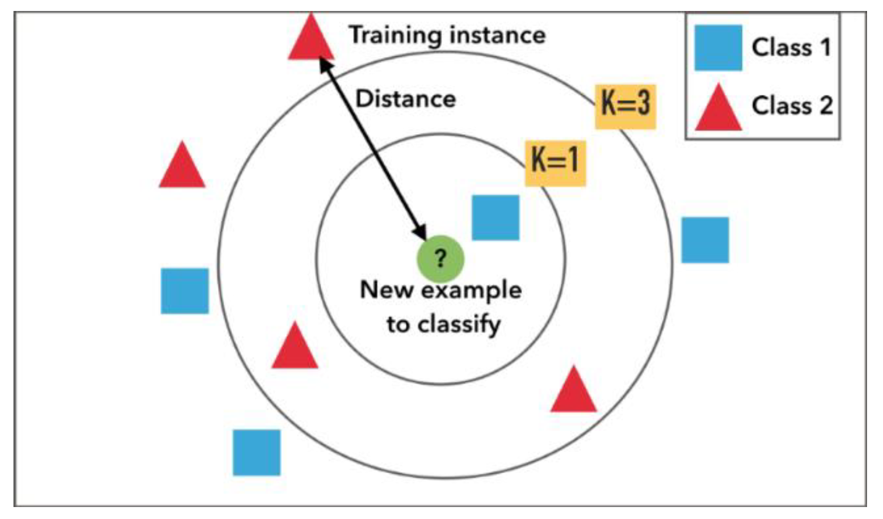
The k-nearest neighbor (kNN) is a supervised ML algorithm that can be used in both classification and regression models. For classification purposes, kNN is a non-parametric method that supports non-linear solutions and can only provide labels as an output. By assuming a value k for the number of nearest neighbors, kNN algorithm identifies the training observations N closest to the new prediction point x, as represented in Figure 6.
Each new observation x is compared to those that already exist in the input dataset by using a distance calculation (such as Euclidean distance, cosine of the angle formed by the two observations, etc.). Then, the class with the smallest distance is assigned to x. The algorithm therefore requires knowing k, the number of neighbors to consider. To choose the right k, the kNN algorithm can be run several times with different values of k. Then, the right k will be the one that has led to the best performance (i.e., the lowest error and the best prediction accuracy).
Studies have proved that kNN is a simple but highly efficient and effective algorithm for solving real-life classification problems (such as the recommendation of movies on NETFLIX) [33,34]. In electrical engineering applications, kNN is mostly use for fault detection and classification but also for power quality classification. The kNN algorithm also has the advantage of being a versatile and easy to understand and implement method with no need for initial assumptions. However, when the volume of samples in the dataset (so-called predictors) increases, the kNN algorithm tends to become slower. Even if there are more precise classification algorithms, kNN remains a first-choice and simple algorithm to model a classification problem and can achieve a high classification accuracy in problems with unknown distributions, while familiarizing with the available database. For this study, the kNN algorithm has been implemented by keeping the Euclidean distance as the employed distance measure. For this study, the Euclidean distance has been employed as the distance measure because of the ease of calculations and possible manual checking of results. Additionally, a limited number of neighbors (k = 5) has been applied.

5.3.2. Decision Tree

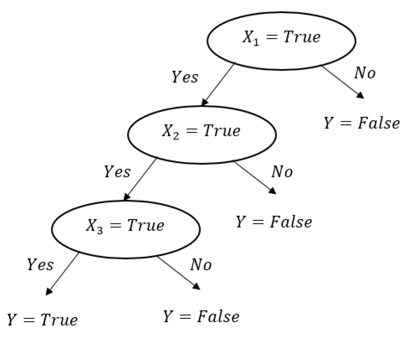
A decision tree (DT) is a supervised ML algorithm used in both regression and classification problems (usually called CART: classification and regression trees). For classification purposes, DT is a widely used non-parametric method, which is based on a hierarchical representation where the end-nodes are the classification and the intermediate nodes are the tests on the properties of the observations (see Figure 7). In other words, building a decision tree is a recursive process, going from the properties (drawn by branches) to the conclusions about an observation (drawn by leaves).
The decision tree starts with a root node (property of X1 in Figure 7) and branches toward possible outcomes. Each of those outcomes leads to additional nodes (property of X2 and X3), which also branch toward other outcomes. In other words, it is a visual representation of the decision-making directly related to the problem to be solved.
A decision tree is a commonly used and highly understandable machine learning method. It is a reliable algorithm for separating a dataset (predictor variables set) into several given classes by providing some clear indications about the most relevant predictors. For classification problems, a DT algorithm does not need much computation and does not rely on functional assumptions (i.e., it is not affected by any non-linearity) while it can build very complex trees and encounter an overfitting problem. Additionally, the creation of optimal decision trees can be obstructed by the presence of dominate classes. DT accuracy reduces, however, when the number of training examples to the number of classes is low. Decision trees are widely used algorithms that give high-quality results with the data, which mostly depends on the conditions [35,36]. In electric power system applications, DT is used in load consumption prediction and load forecasting, preventive and corrective control, power systems security assessment, etc. [37]. The DT algorithm, in this study, is an adjusted binary classification decision tree.

5.3.3. Logistic Regression

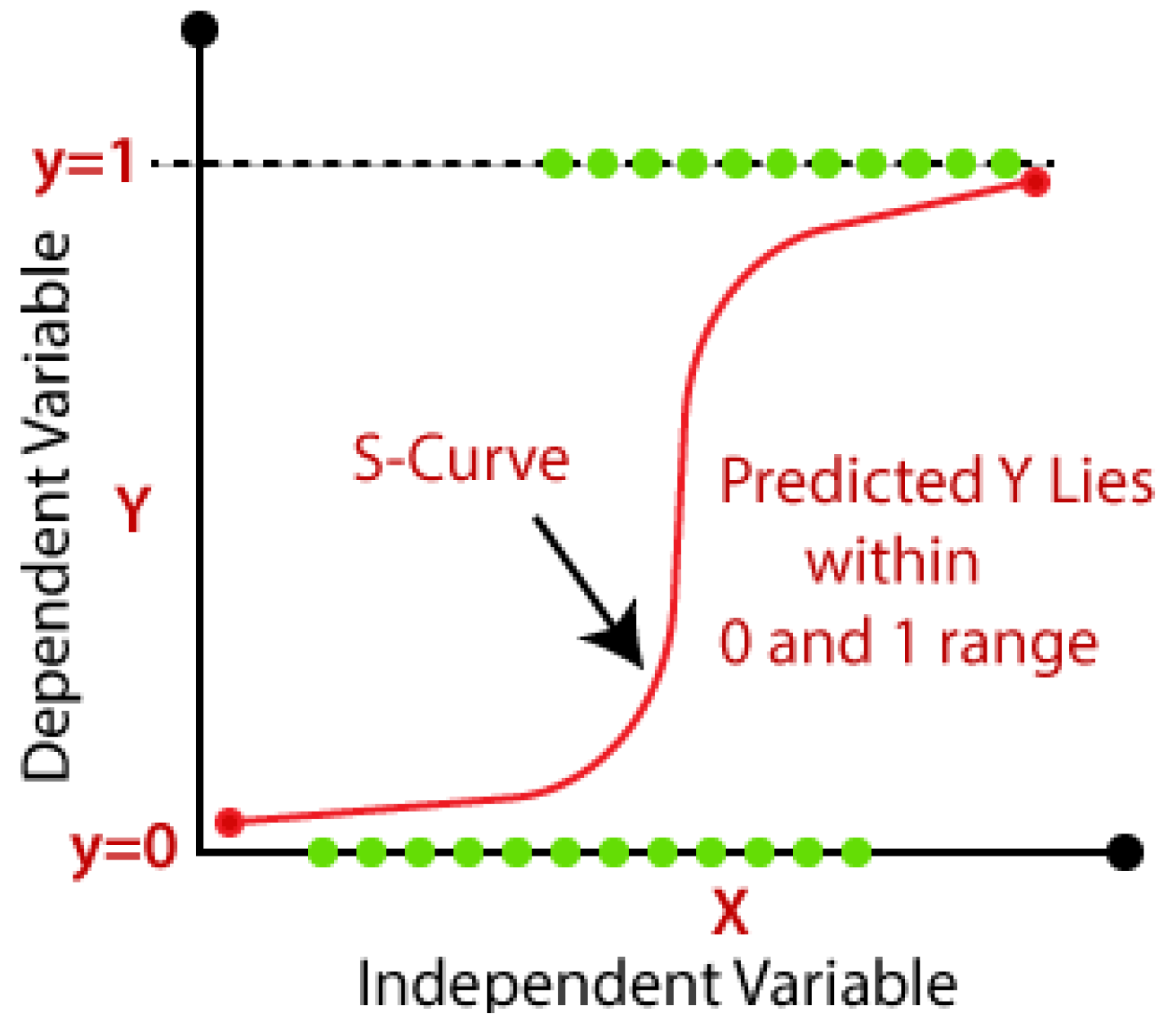
Logistic regression (LR) is a parametric model that supports linear solutions and can derive to a high confidence level (regarding its prediction). LR is a powerful algorithm for finding boundaries between two classes. Mathematically speaking, an LR algorithm uses regression to predict the probability (between 0 and 1) of a new observation x to be classified into y, a given class (see Figure 8).
A mathematical representation of LR will be made here. Considering the two-class classification problem of this paper, an analogy can be made between the labels and the output classes as shown in Table 2.
The output h θ ( x )   of a logistic regression model (i.e., the probability of a new observation x to be classified into a class y) will be bounded as below:
0 h θ ( x ) 1  
{ I f h θ ( x ) 0.5 : p r e d i c t   y = 1 I f h θ ( x ) < 0.5 : p r e d i c t   y = 0
For this classification problem, the probability value h θ ( x ) can be calculated by using a sigmoid function g (S-curve function to map predictions to probabilities):
g ( u ) = 1 1 + e u
Then h θ ( x ) can be written as bellow:
h θ ( x ) = g ( θ T x )  
where the input of the sigmoid function (u) is the weighted sum of the input predictors (x).
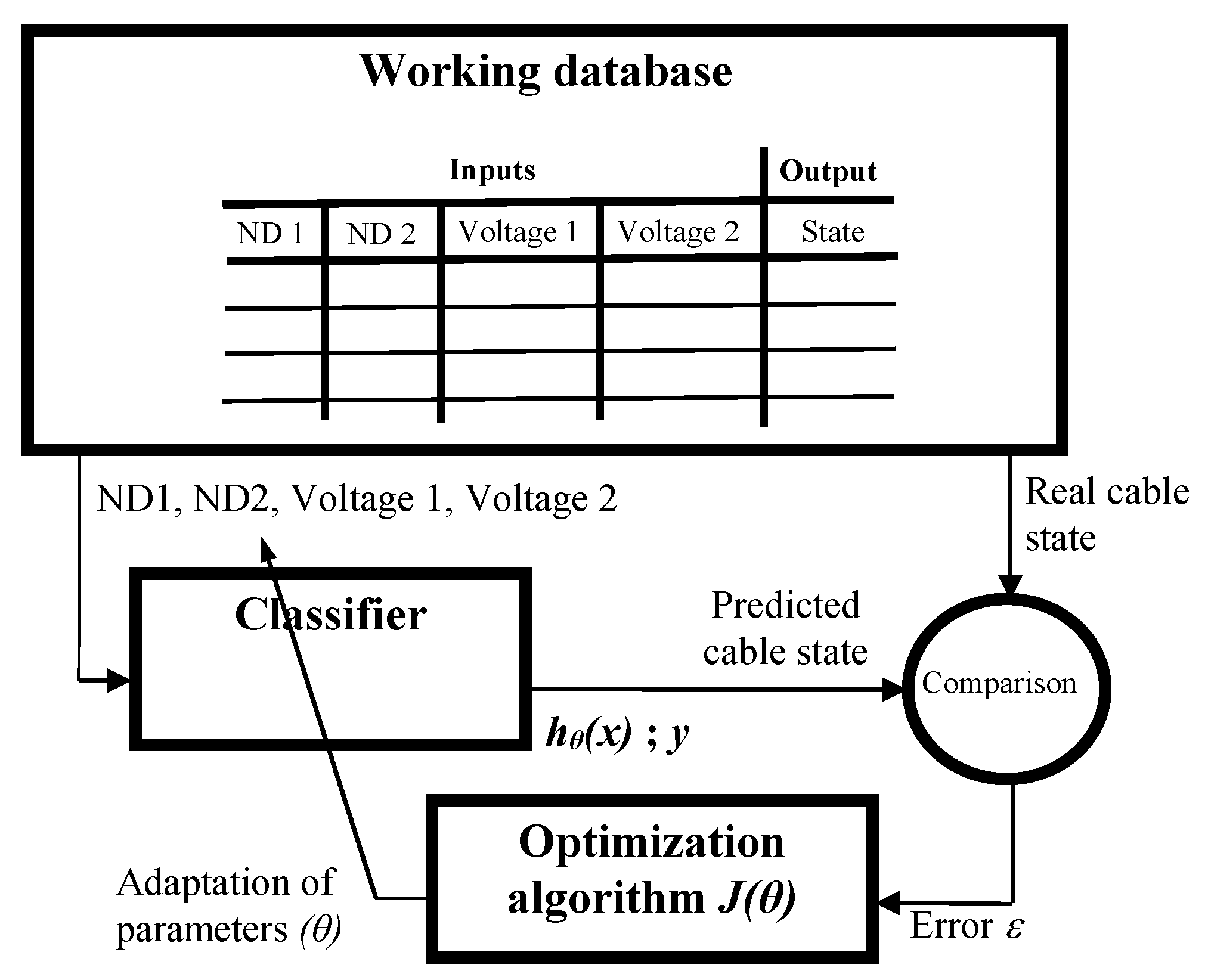
The key point is then to find the right values for parameters θ (θ being a vector of the same size as the observation vector x) by solving a minimization problem:
min θ J ( θ )  
with
J ( θ ) = 1 M m = 1 M c o s t ( h θ ( x ( m ) ) , y ( m ) )
where J is a cost function, M is the total number of observations in the dataset and cost is the quadratic classification error that is expressed as follows [39]:
c o s t ( h θ ( x ) , y ) = 1 2 ( 1 1 + e ( θ T x ) y ) 2  
c o s t ( h θ ( x ) , y ) = { log ( h θ ( x ) )   i f   y = 1 log ( 1 h θ ( x ) )   i f   y = 0  
The cost function to be minimized will be equal to:
J ( θ ) = 1 M m = 1 M [ y ( m ) log ( h θ ( x ( m ) ) ) + ( 1 y ( m ) ) log ( 1 h θ ( x ( m ) ) ) ]
The logistic regression method is the go-to method for binary classification problems (problems with two class values). LR is easy to implement, fast and very efficient to train. The LR algorithm gives good accuracy for simple datasets and the provided model coefficients can be interpreted as indicators of predictor importance. LR has the advantage of being less likely to lead to over-fitting, except in high dimensional datasets. Logistic regression methods are used, in electrical engineering, for electricity monitoring, visualization and prediction but also for fault detection in renewable energy production [40].

6. Application

6.1. Presentation of the Monitored Low-Voltage Distribution Network

The LV distribution network studied in this paper is presented in Figure 9. Having a radial topology, it consists of 18 nodes, each one (except node 1, i.e., the slack bus) connected to a customer (Ci) with photovoltaic panels (so-called prosumers). The LV network is part of Flobecq town distribution system in Belgium [14,16], where each prosumer is equipped with a smart meter (SM). The SM simultaneously records, at each node and for each quarter of an hour, the PV generation, the injection and the consumption. Using those measured energy values, the system powers P (active power) and Q (reactive power) are calculated (Appendix B shows the associated lengths of the lines).
For the sake of simplicity, the analysis of this paper is carried out on a portion of the network shown in Figure 9, which is in the upward direction of node 3. The input node (i.e., node 2) is connected to customer C1 while the output node (i.e., node 3) is connected to customer C2. The first node (i.e., node 1) connected to the secondary side of the transformer is supposed to be at the 230 V reference value. In this study, a month of SM data is used to build the dataset. For each day, 96 measurements are made. The total number of observations is thus equal to 2880 measurements (i.e., 30 × 96). Those 2880 observations are created while ensuring uniformity of the two classes in the synthetic dataset. Table 3 shows how the cable states are distributed in the working database.

6.2. Training and Validation Sets

Supervised machine learning algorithms consist of two phases—a training phase and testing phase. During the training phase, the training samples and the class labels of these samples are stored in a subset. The algorithm to learn and to create the right output from the data uses this subset. While training, the algorithm modifies the training parameters. In this phase, the algorithm is said to be learning. During the testing phase, the remaining observations from the original dataset are stored in a subset without the associated output. Then, a prediction is made on those samples to check how well the algorithm predicts the desired output.
To fit those two phases, the original dataset has been reduced in two subsets: the training subset and the test subset. The training subset is used to train the algorithm and the test subset is used to make some predictions for the resulting model validation. To select the observations in each data subset, a random logical selection was made. Table 4 and Table 5 summarize the repartition of the data used in each classification algorithm.
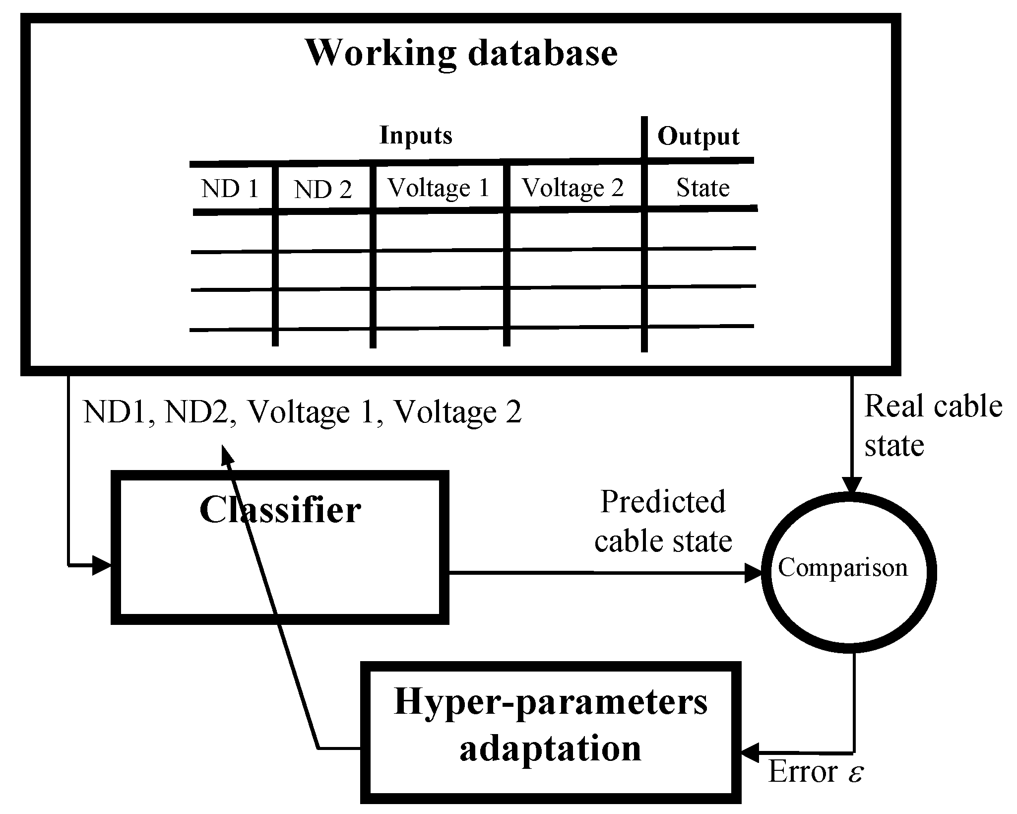
As explained in Section 2, the main purpose of this work is to identify if the monitored cable section (i.e., the one between nodes 2 and 3) is either in the healthy working condition (class H) or has any insulation wear (class M). This classification will be made by various ML methods using an input dataset built from the provided smart meter data and computed nodal voltage variations. Figure 10 presents the flowchart of the implemented tool for solving that classification problem while Figure 11 and Figure 12 show the specified classification process for each implemented algorithm.

6.3. Test Cases

In order to evaluate the performance of the proposed framework, two cases are considered as follows.

6.3.1. Case 1: Impact of the Net Demand and the Thickness Variation

The first application case will evaluate the impact of the net demand and the thickness variation on the model training and the prediction result. In this case, the net demand (ND) and the nodal voltage (V) of both the input node (named ND1 and V1) and output node (named ND2 and V2) are given to the classification input dataset. This helps the algorithm in its learning process. The algorithm will understand if any variation in the data is related to a cable degradation (based on the net demand/voltage level compromise) or to the client net demand.

6.3.2. Case 2: Impact of the Net Demand on the Prediction Result

The second application case will evaluate the impact of the net demand on the model training and the prediction result. In this scenario, only the nodal voltage (V) of both input node (V1) and output node (V2) are given to the classifier in the training subset. The idea is to evaluate if the algorithm can really distinguish between the effects of thickness variation independent of the net demand variation.

7. Results and Discussion

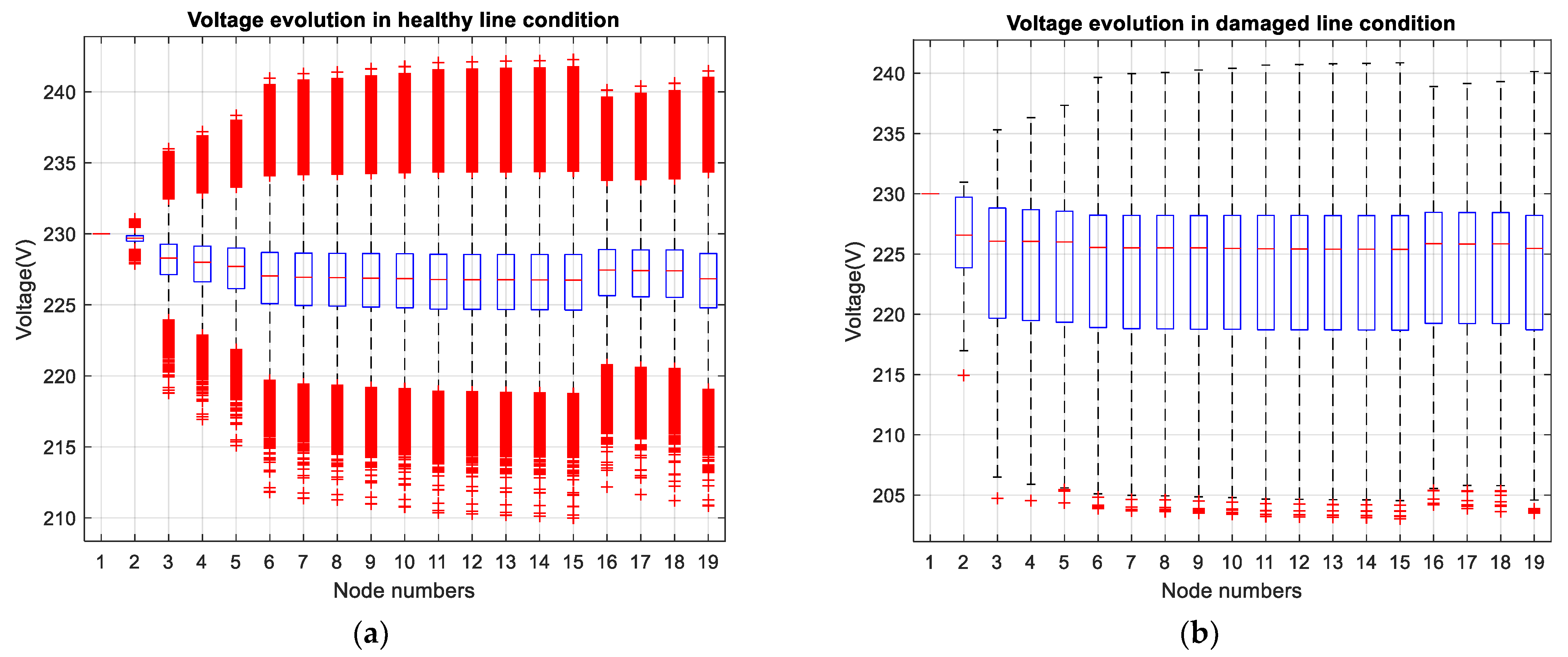
A first investigation is carried out to find the nodal voltage variation range of the feeder in a healthy cable condition (knowing that the maximum ND is associated to minimum voltage). The obtained values are limited to [210.19, 242.2734] Volts as shown in Figure 13a. In addition, Figure 13b presents the nodal voltages for moderately degraded cable located in the line between nodes 2 and 3. It should be noted that the extreme degradation scenarios as studied in [6] have not been considered in this work. Moreover, the severe faults (extreme degradation scenarios) are easier to observe and detect. The interest in this study is focused more on the detection of the cable at the beginning of degradation process, which will be useful in managing cable maintenance and in anticipating the occurrence of severe faults or outage. Hence, the moderately degraded cable condition is linked to a soft fault degradation, which is not necessarily in breakage conditions but just introduces significant variations in the voltage profile.
In the boxplots of nodal voltage profiles shown in Figure 13, the red positive signs demonstrate the outliers of the voltages in the created scenarios. The outliers in Figure 13a are related to the prosumers ND demand variations while those in Figure 13b are due to the nonlinear equation of the insulation conductance (1/Riso) applied in the NRLF computation. As it can be understood, the increase in insulation conductance (1/Riso) can lead to the voltage drops shown by the outliers.
Table 6 and Table 7 show the prediction results obtained by the studied classification techniques in case 1 and case 2.
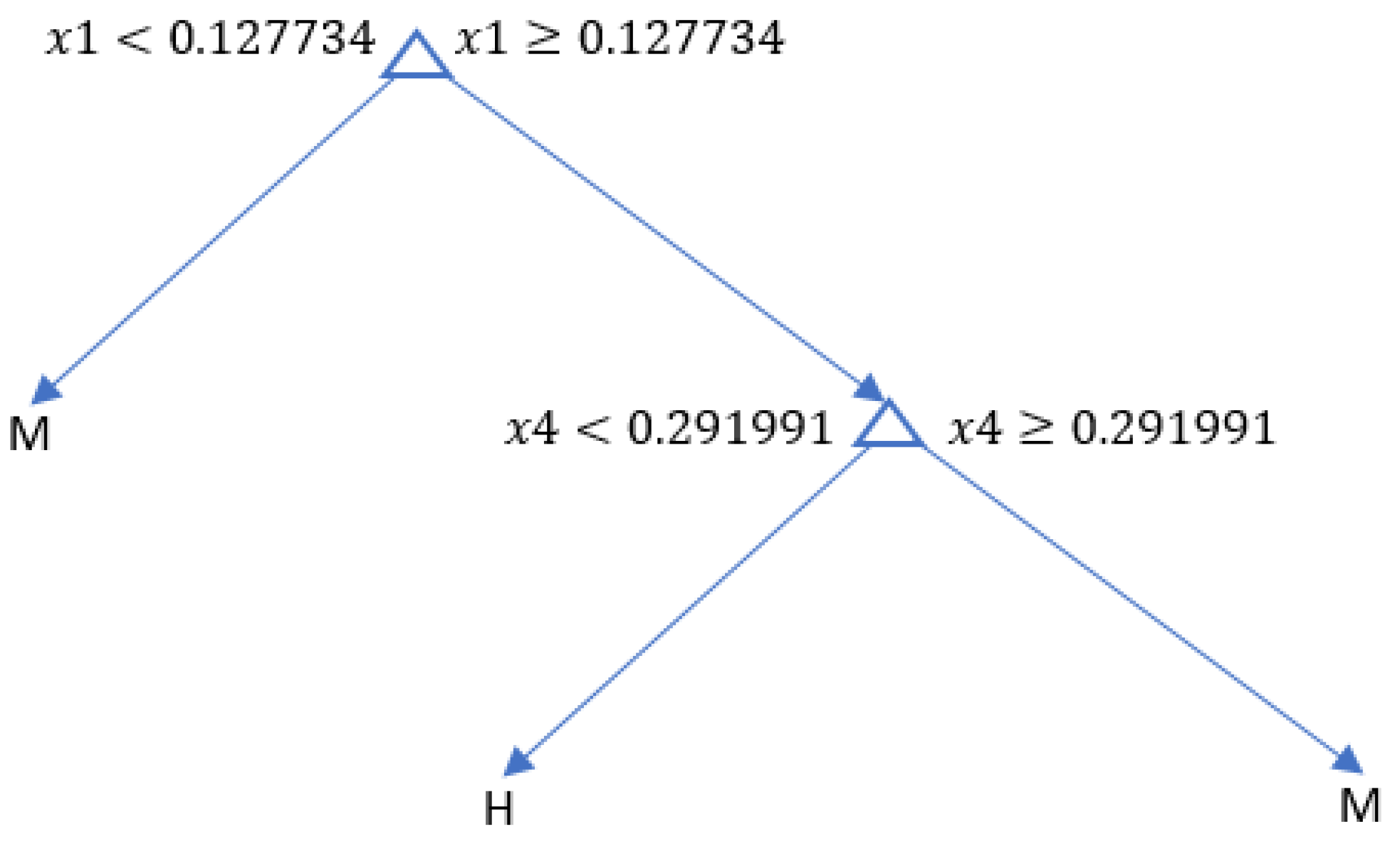
In Table 6, it can be observed that LR and DT demonstrate good accuracies in the prediction process in case 1 (model trained with ND variations and nodal voltage profiles) while kNN performance is in a lower level. For the case 2, where the net demand (DT) is missing, it can be seen that the implemented algorithms lost performance. Therefore, the ND is an important predictor (input variable) for the classifier, as well as the voltage profiles. This is due to its unneglected impact on the nodal voltage variation range [6]. The constructed tree for DT method is shown in Figure 14 (corresponding to case 1). It reveals that normalized input ND profiles (named x1) will affect the prediction process as well as the normalized output voltage profile (named x4). As a result, the LR and DT lead to predictions with high accuracies in case 1.
Table 8 gives the related training and prediction accuracy for each studied classification method. By comparing these results, it can be concluded that the LR and decision tree are great binary classification tools, while the kNN method leads to less accurate predictions.
Figure 15 represents the confusion matrix of LR and DT methods for the first application case in order to visualize the quality of the classifiers output (see if the predictions really match the real associated classes for validating the prediction counts in Table 6) in a three-dimensional plot. In Figure 15, the axes yPred and yvalid correspond, respectively, to the outputs of the classifier (the predictions) and to the known cable conditions (real classes from the original dataset). Only a few damaged cable conditions could not be predicted with either LR or DT algorithms (small blue block corresponding to 30 observations in Figure 15a and four observations in Figure 15b).
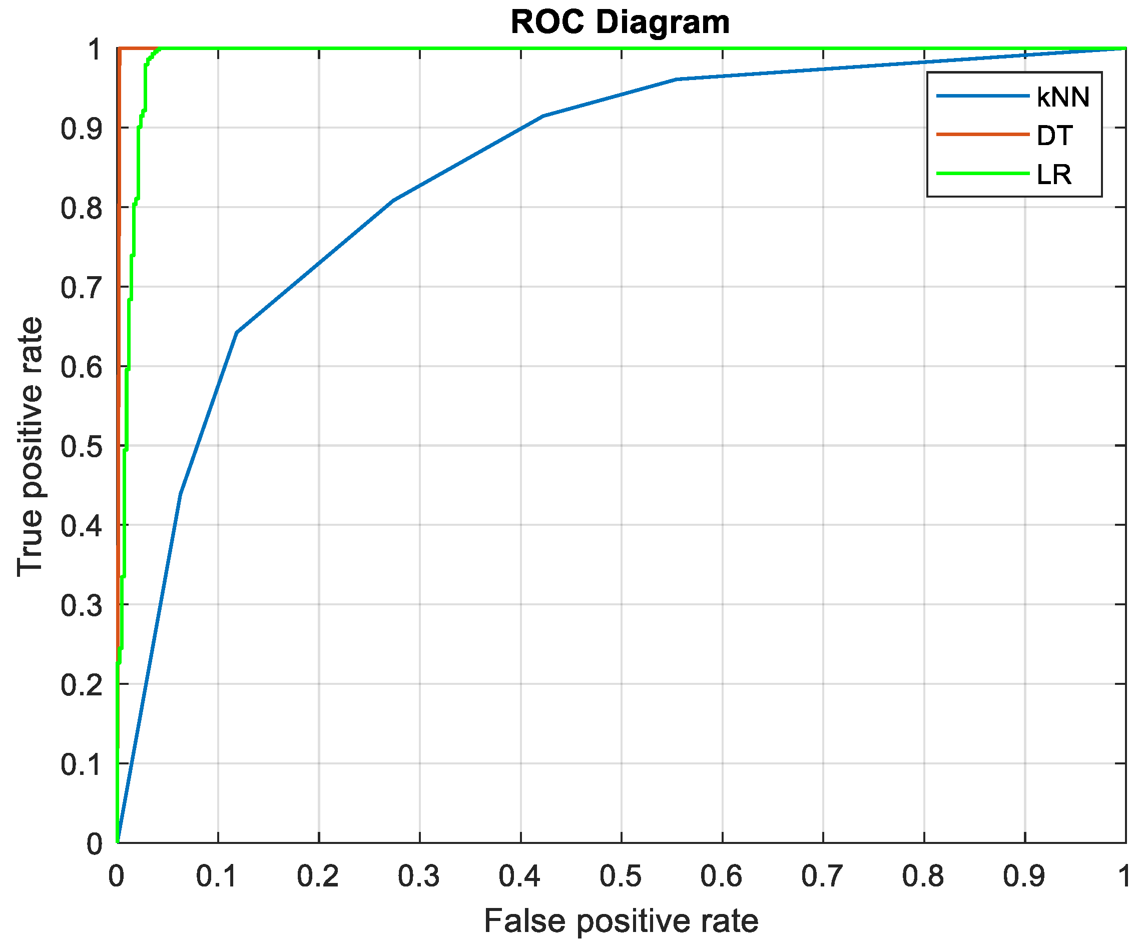
Figure 16 shows the ROC (receiver operating characteristic) diagram representation of the prediction, which shows the ratio between the true positive (sensitivity) and the false positive (specificity) outputs of the classifier. It is the curved diagram of the classifier’s accuracy (in Table 8). Knowing that the closer the curve is to a 45-degree diagonal of the ROC space, the less accurate the prediction result, it can be concluded that kNN is clearly the least efficient algorithm in the studied application case.
The conducted simulations on various degrees of insulation wear reveal interesting information about the added value of data-driven approaches for the cable condition assessment. Particularly, this work demonstrates the ability of different classification algorithms to identify, on the basis of only ND and voltage variation, the LV network cable condition assessment.
However, this presented work should not be directly extended for other practical applications or be generalized, for two reasons. Firstly, the resistance of the insulation material is calculated (in Section 3) within consideration of some LV cable electrical properties specific to each manufacturer. Secondly, machine-learning techniques have been developed here for the degradation detection in operating domains where the causes of observed variations are difficult to interpret. Hence, to avoid a direct median separation in the observations, the input database has been built (in Section 5.1) by excluding the cases of extreme degradation scenarios (severe faults) because they are easily detected without any advanced techniques.

8. Conclusions

In this study, a machine learning-based framework is proposed for the identification of low voltage cable degradation due to the insulation material wear. To this end, a probabilistic tool was first developed to generate scenarios for the uncertain nature and degree of the cable insulation degradation. Those scenarios were then associated with the load demand and PV generation variations and used to build the nodal voltage database by performing probabilistic load flow calculations. Different supervised learning methods were finally applied to the generated database. In the first (training) stage, the studied classification methods learned from the given inputs, its associated cable condition status in order to be able to predict, in the second (test) phase, the cable condition corresponding to each given network operating point. The comparisons between the implemented classifiers show that logistic regression and decision tree approaches are powerful binary classification tools with 97.917% and 99.884% accuracy performance, respectively, while the k-nearest neighbors method could not provide accurate predictions. The conducted study reveals the added value of such a data-driven approach for the cable condition assessment.
The interest of this work is to set up a tool that can assist the distribution system operators (DSOs) in an effective and timely predictive maintenance of the LV distribution network, avoiding the costly solutions. Indeed, the obtained result offers promising perspectives for the early detection of cable degradation by combining ML approaches, load demands profiles and smart meter (SM) measurements.
For future work, this research will extend the current model to a complete network, on the basis of cross nodal learning (learning between the models of each line section or cables in the network). The current study is the first step towards a global and generalized (e.g., by considering the type of cable as one of the classifier parameters) data-based early identification of electrical low voltage cable degradation due to insulation wear, using machine learning tools.
Author Contributions

All the authors have contributed equally for this research article, from the conceptualization, methodology, implementation, analysis, discussion, validation, writing to review and editing. All authors have read and agreed to the published version of the manuscript.

Funding

This research received no external funding.

Institutional Review Board Statement

Not applicable.

Informed Consent Statement

Not applicable.

Data Availability Statement

We applied our proposed approach to the Smart Meter measurements database (and LV network technical information) which are part of the local DSO private property.

Acknowledgments

The authors would like to thank ORES, Belgian Distribution System Operator, for providing them with the required data.

Conflicts of Interest

The authors declare no conflict of interest.

Appendix A

Figure A1. Global flowchart of the implemented process.
Energies 14 02852 g0a1

Appendix B

Table B1. Line lengths of the studied LV network.
Line Between:Length (in Km)Line Between:Length (in Km)
Node 1 and Node 2 0.046Node 10 and Node 110.044
Node 2 and Node 3 0.273Node 11 and Node 120.01
Node 3 and Node 40.062Node 12 and Node 130.015
Node 4 and Node 50.063Node 13 and Node 140.014
Node 5 and Node 60.194Node 14 and Node 150.041
Node 6 and Node 70.026Node 5 and Node 16 0.396
Node 7 and Node 80.011Node 16 and Node 170.093
Node 8 and Node 90.025Node 17 and Node 180.117
Node 9 and Node 100.021Node 7 and Node 190.119

References

  1. Norme Française NF C 15-100 (Décembre 2002). Installations Electriques à Basse Tension. Available online: http://alternatif33.free.fr/NFC15100_2002.pdf (accessed on 23 September 2020).
  2. Codjo, E.L.; Vallée, F.; Francois, B. Impact of the line resistance statistical distribution on a probabilistic load flow computation. In Proceedings of the 2020 6th IEEE International Energy Conference (ENERGYCon), Gammarth, Tunisia, 28 September–1 October 2020; pp. 637–642. [Google Scholar]
  3. Bakhshideh Zad, B.; Hasanvand, H.; Lobry, J.; Vallée, F. Optimal reactive power control of DGs for voltage regulation of MV distribution systems using sensitivity analysis method and PSO algorithm. Int. J. Electr. Power Energy Syst. 2015, 68, 52–60. [Google Scholar] [CrossRef]
  4. Bakhshideh Zad, B.; Lobry, J.; Vallée, F. A centralized approach for voltage control of MV distribution systems using DGs power control and a direct sensitivity analysis method. In Proceedings of the 2016 IEEE International Energy Conference, Leuven, Belgium, 4–8 April 2016. [Google Scholar]
  5. Salivon, T. Vieillissement Thermique D’isolants en PVC et PELX de Câbles Electriques en Environnement Automobile. Ph.D. Thesis, Ecole Nationale Supérieure d’arts et Métiers—ENSAM, Paris, France, 2017. [Google Scholar]
  6. Techni-Tool Company. The Complete Guide to Electrical Insulation Testing; Ensto Finland OyEnsio. Available online: https://www.instrumart.com/assets/Megger-Guide-to-Insulation-Testing.pdf (accessed on 4 January 2020).
  7. Kang, S.-D.; Kim, J.-H. Investigation on the insulation resistance characteristics of Low Voltage cable. Energies 2020, 13, 3611. [Google Scholar] [CrossRef]
  8. Kruizinga, B.; Wouters, P.A.A.F.; Steennis, E.F. Fault development on water ingress in damaged underground Low Voltage cables with plastic insulation. In Proceedings of the 2015 IEEE Electrical Insulation Conference (EIC), Seattle, WA, USA, 7–10 June 2015; pp. 309–312. [Google Scholar]
  9. Kruizinga, B.; Wouters, P.A.A.F.; Steennis, E.F. Comparison of polymeric insulation materials on failure development in low-voltage underground power cables. In Proceedings of the 2016 IEEE Electrical Insulation Conference (EIC), Montreal, QC, Canada, 19–22 June 2016; pp. 444–447. [Google Scholar]
  10. Helmholt, K.A.; Groote Schaarsberg, M.; Broersma, T.; Morren, J.; Kruizinga, B.; Wouters, P.A.A.F.; Steennis, E.F.; Baldinger, F. A structured approach to increase situational awareness in low voltage distribution grids. In Proceedings of the 2015 IEEE Eindhoven PowerTech, Eindhoven, The Netherlands, 29 June–2 July 2015; pp. 1–6. [Google Scholar]
  11. Csányi, G.M.; Tamus, Z.Á.; Varga, Á. Impact of Distributed Generation on the Thermal Ageing of Low Voltage Distribution Cables. In Proceedings of the 8th Doctoral Conference on Computing, Electrical and Industrial Systems (DoCEIS), Costa de Caparica, Portugal, 3–5 May 2017; pp. 251–258. [Google Scholar]
  12. Csányi, G.M.; Tamus, Z.Á.; Kordás, P. Effect of Enhancing Distribution Grid Resilience on Low Voltage Cable Ageing. In Technological Innovation for Resilient Systems, Proceedings of the Doctoral Conference on Computing, Electrical and Industrial Systems (DoCEIS), 29 March 2018; Springer: Cham, The Netherland, 2018; pp. 300–307. [Google Scholar]
  13. Csányi, G.M.; Bal, S.; Tamus, Z.Á. Dielectric Measurement Based Deducted Quantities to Track Repetitive, Short-Term Thermal Aging of Polyvinyl Chloride (PVC) Cable Insulation. Polymers 2020, 12, 2809. [Google Scholar] [CrossRef] [PubMed]
  14. Codjo, E.L.; Bakhshideh Zad, B.; Vallée, F.; François, B. Analysis of Low-Voltage Network Sensitivity to Voltage Variations Due to the Insulation Wear. In Proceedings of the 55th International Universities Power Engineering Conference (UPEC), Turin, Italy, 1–4 September 2020. [Google Scholar]
  15. Klonari, V.; Toubeau, J.-F.; De Grève, Z.; Durieux, O.; Lobry, J.L.; Vallée, F. Probabilistic simulation framework for balances and unbalanced low voltage networks. Int. J. Electr. Power Energy Syst 2016, 82, 439–451. [Google Scholar] [CrossRef]
  16. Conti, S.; Raiti, S. Probabilistic load flow using Monte Carlo techniques for distribution networks with photovoltaic generators. Sol. Energy 2007, 81, 1473–1481. [Google Scholar] [CrossRef]
  17. Klonari, V.; Bakhshideh Zad, B.; Lobry, J.; Vallée, F. Application of voltage sensitivity analysis in a probabilistic context for characterizing low voltage network operation. In Proceedings of the 2016 International Conference on Probabilistic Methods Applied to Power Systems, Beijing, China, 16–20 October 2016. [Google Scholar]
  18. Bakhshideh Zad, B.; Lobry, J.; Vallée, F. Impacts of the model uncertainty on the voltage regulation problem of medium-voltage distribution systems. Iet Gener. Transm. Distrib. 2018, 12, 2359–2368. [Google Scholar] [CrossRef] [Green Version]
  19. Bakhshideh Zad, B.; Toubeau, J.-F.; Lobry, J.; Vallée, F. Robust voltage control algorithm incorporating model uncertainty impacts. Iet Gener. Transm. Distrib. 2019, 13, 3921–3931. [Google Scholar] [CrossRef] [Green Version]
  20. Klerx, M.H.P. Condition Assessment of Low Voltage Distribution Grids; Technische Universiteit Eindhoven: Eindhoven, The Netherlands, 2020. [Google Scholar]
  21. Asadi Majd, A.; Samet, H.; Ghanbari, T. k-NN based fault detection and classification methods for power transmission systems. Prot. Control Mod. Power Syst. 2017, 2, 1–11. [Google Scholar] [CrossRef] [Green Version]
  22. Baskar, D.; Selvam, P. Machine Learning Framework for Power System Fault Detection and Classification. Int. J. Sci. Technol. Res. 2019, 9. [Google Scholar]
  23. Sapountzoglou, N. Fault Detection and Isolation for Low Voltage Distribution Grids with Distributed Generation; Université Grenoble Alpes: Grenoble, France, 2016. [Google Scholar]
  24. Ndeye, L.; Flaus, J.-M.; Adrot, O. Review of Machine Learning Approaches in Fault Diagnosis applied to IoT System. In Proceedings of the 2019 International Conference on Control, Automation and Diagnosis ICCAD’19, Grenoble, France, 2–4 July 2019. [Google Scholar]
  25. Huo, Y.; Prasad, G.; Lampe, L.; Leung, C.V. Smart-grid monitoring: Enhanced machine learning for cable diagnostics. In Proceedings of the 2019 IEEE International Symposium on Power Line Communications and Its Applications (ISPLC), Prague, Czech Republic, 3–5 April 2019; pp. 1–6. [Google Scholar]
  26. Khan, M.A.; Kim, J. Toward Developing Efficient Conv-AE-Based Intrusion Detection System Using Heterogeneous Dataset. Electronics 2020, 9, 1771. [Google Scholar] [CrossRef]
  27. Wenshuo, T.; Flynn, D.; Brown, K.; Valentin, R.; Zhao, X. The Application of Machine Learning and Low Frequency Sonar for Subsea Power Cable Integrity Evaluation. In Proceedings of the OCEANS 2019 MTS/IEEE SEATTLE, Seattle, WA, USA, 27–31 October 2019; pp. 1–6. [Google Scholar]
  28. Toubeau, J.-F.; Bakhshideh Zad, B.; Hupez, M.; De Grève, Z.; Vallée, F. Deep reinforcement learning-based voltage control to deal with model uncertainties in distribution networks. Energies 2020, 13, 3928. [Google Scholar] [CrossRef]
  29. BICC Cables Ltd. Electric Cables Handbook, 3rd ed.; Wiley-Blackwell: Hoboken, NJ, USA, 1997. [Google Scholar]
  30. Saadat, H. Power System Analysis; McGraw-Hill: New York, NY, USA, 1999. [Google Scholar]
  31. Shalev-Shwartz, S.; Ben-David, S. Understanding Machine Learning: From Theory to Algorithms; Cambridge University Press: Cambridge, UK, 2014. [Google Scholar]
  32. Noteworthy the Journal Blog. A Quick Introduction to K-Nearest Neighbors Algorithm. 2017. Available online: https://blog.usejournal.com/a-quick-introduction-to-k-nearest-neighbors-algorithm-62214cea29c7 (accessed on 19 November 2020).
  33. Chen, G.; Shah, D. Explaining the Success of Nearest Neighbor Methods in Prediction. Found. Trends Mach. Learn. 2018, 10, 105–199. [Google Scholar] [CrossRef]
  34. Imandoust, S.B.; Bolandraftar, M. Application of K-Nearest Neighbor (KNN) Approach for Predicting Economic Events: Theoretical Background. Int. J. Eng. Res. Appl. 2013, 3, 605–610. [Google Scholar]
  35. Carnegie Mellon University—School of Computer Science. Artificial Intelligence: Representation and Problem Solving. Introduction to Learning & Decision Trees. 2007. Available online: https://www.cs.cmu.edu/afs/cs/academic/class/15381-s07/www/slides/041007decisionTrees1.pdf (accessed on 23 November 2020).
  36. Great Learning Blog. Decision Tree Algorithm Explained with Examples. 2020. Available online: https://www.mygreatlearning.com/blog/decision-tree-algorithm/ (accessed on 23 November 2020).
  37. Liu, C.; Rather, Z.; Chen, Z.; Bak, C.L. An overview of decision tree applied to power systems. Int. J. Smart Grid Clean Energy 2013, 2, 413–419. [Google Scholar] [CrossRef] [Green Version]
  38. JavaTpoint. Linear Regression vs Logistic Regression. 2018. Available online: https://www.javatpoint.com/linear-regression-vs-logistic-regression-in-machine-learning (accessed on 25 November 2020).
  39. Andrew, N. Machine Learning. Available online: https://www.coursera.org/lecture/machine-learning/classification-wlPeP (accessed on 14 September 2020).
  40. Ansari, M.; Srivastava, K.; Kaluri, R. Electricity Monitoring, Visualization and Prediction Using Logistic Regression. 2017. Available online: https://www.researchgate.net/publication/319523536_Electricity_Monitoring_Visualization_and_Prediction_using_Logistic_Regression (accessed on 4 January 2021). [CrossRef]
Figure 1. Series model of a healthy line [14].
Energies 14 02852 g001
Figure 2. Model of a line having a damaged cable insulation [14].
Energies 14 02852 g002
Figure 3. Equivalent model of the damaged line.
Energies 14 02852 g003
Figure 4. Flowchart of the synthetic creation of the database.
Energies 14 02852 g004
Figure 5. Visualization of supervised machine learning approach.
Energies 14 02852 g005
Figure 6. kNN representation [32].
Energies 14 02852 g006
Figure 7. Decision tree representation.
Energies 14 02852 g007
Figure 8. Logistic regression representation [38].
Energies 14 02852 g008
Figure 9. Topology of the monitored LV distribution network.
Energies 14 02852 g009
Figure 10. Flowchart of the classification process: from the model training to the prediction.
Energies 14 02852 g010
Figure 11. Classification process specified to decision tree (DT) and k-nearest neighbor (kNN) algorithms.
Energies 14 02852 g011
Figure 12. Classification process specified to logistic regression (LR) algorithm.
Energies 14 02852 g012
Figure 13. Boxplots of nodal voltages obtained by the load flow calculations (a) for feeder in a healthy cable condition, and (b) for feeder with a moderately damaged cable located in the line between nodes 2 and 3.
Energies 14 02852 g013
Figure 14. Constructed decision tree in case 1.
Energies 14 02852 g014
Figure 15. Confusion matrix of the prediction result: logistic regression method (a) and decision tree method (b).
Energies 14 02852 g015
Figure 16. ROC diagram of the prediction result for k-nearest neighbors (kNN), decision tree (DT) and logistic regression (LR) methods.
Energies 14 02852 g016
Table 1. Label table for the observations.
Cable StateLabelsDescription
No insulation wearHH for Healthy
Insulation wearMM for Medium
Table 2. Analogy between labels and classes.
State of the LineLabelsClass in LR
No insulation wearH1 for the positive class
Insulation wearM0 for the negative class
Table 3. Observation in the working database.
Observations StateNumber of Observations
H1441
M1439
Total2880
Table 4. Partition of the data.
DatabasePercentageObservations
Working database100%2880
Training subset70%2016
Test subset30%864
Table 5. Distribution of the observations in each subset.
Observations StateWorking DatabaseTraining SubsetTesting Subset
H14411008441
M14391008423
Total28802016864
Table 6. Prediction results for application case 1.
Observations StateReal StatekNNDTLR
H433468434447
M431396430417
Total864864864864
Table 7. Prediction results for application case 2.
Observations StateReal StatekNNDTLR
H433299454524
M431565410340
Total864864864864
Table 8. Training and prediction results accuracy for application case 1.
AlgorithmsTraining ErrorPrediction Error (%)Accuracy (%)
kNN0.1542723.26476.736
DT00.11699.884
LR02.08397.917
Publisher’s Note: MDPI stays neutral with regard to jurisdictional claims in published maps and institutional affiliations.