Abstract
Equivalent power system impedance is an important electrical quantity from many points of view. Areas in which this parameter plays an important role include, in particular: Voltage stability analysis, power quality, or fault condition analysis. Power system impedance estimation in real operation conditions can be performed by one of the non-invasive methods described by different authors. This paper aims to investigate and compare seven different methods for power system impedance estimation based on voltage and current variations measurement. After a brief description of selected methods, these methods were applied for power system impedance estimation in the case of two simple simulation tests and then in the case of three real measured data. Voltage and current changes used for power system impedance estimation in real conditions were measured in high voltage (HV) and medium voltage (MV) substations feeding steel mill with the electric arc furnace (EAF) operation. As the results presented in this paper have shown, not all of the methods analyzed are suitable for determining the power system impedance based on the fast step changes of voltage and current that occur, for example, during an EAF operation. Indeed, some of the tested methods were originally designed to determine the power system impedance from changes in voltages and currents recorded at steady state.
1. Introduction
Measuring and determining the power system impedance in real conditions is an ever-evolving field of research. The reason is the fact that there is currently no uniform and reliable methodology for determining the actual value of the power system impedance. In the case of power system impedance, or Thevenin impedance (TI), it is necessary to distinguish at least between two of its types. The first type of TI represents the power system equivalent impedance in the case of steady-state conditions. This type of TI is important to know, for example, for purposes of evaluation of the power system voltage or static stability. The second type of TI represents the power system equivalent impedance in the case of large rapid change in operating conditions, such as in the case of fault occurrence. The difference between these two types of TI depends on the influence of the behavior of synchronous and asynchronous machines as well as of a load in general. In the case of steady-state conditions, the behavior (or impedance) of synchronous and asynchronous machines as well as of a load, in general, is different as in the case of large rapid voltage change occurrence, for example during close-to-fault conditions. On the other hand, in the case of nodes electrically far from synchronous and asynchronous machines, these two types of Thevenin impedances become one. An influence of different load types (modeled as constant impedance, constant current, or constant power) to the power system (Thevenin) impedance monitoring is discussed in [1]. The effect of load active and reactive power change on the power system’s TI is discussed in [2]. Few works are dealing with the power system impedance evaluation for purposes of voltage stability analysis using different techniques [3,4,5,6]. Analysis of the influence of wind power station on the power system’s Thevenin equivalent impedance is discussed in [7]. In [8], authors describe the method for TI estimation of concerned power system areas using data measured with phasor measurement units (PMU) and the impedance matrix of the known part of the power system.
Knowing the actual value of the power system impedance during specific or standard operating conditions also has a major impact in assessing the feedback effects of new and existing electrical equipment on power quality. For example, static var compensators (SVC) or other types of flexible alternating current transmission systems (FACTS) are often used to eliminate the negative impact of other electrical devices on the level of voltage quality. Suppliers of such FACTS devices generally declare the positive effect of these devices on power quality with respect to the maximum value of the power system impedance (mainly with respect to short-circuit impedance or short-circuit power).
The maximum, as well as the minimum, short-circuit power, as well as the short-circuit impedance in accordance with [9], represent theoretical values determined by calculation for network configurations leading to maximum or minimum short-circuit power, or to minimum short-circuit currents. The results of the comparison of the value of short-circuit power (or power system impedance) in different nodes of the power system during island operation presented in [10] showed a correlation between theoretical calculations performed according to [9] and values determined from the measurement of voltage and current jumps. However, in the case of real operation, the actual value of the equivalent short-circuit impedance of the network varies between the values determined for the minimum and maximum short-circuit current (power).
Non-invasive methods of determining the actual value of the power system impedance are mostly based on determining the voltage change at a given location of the network due to measured current change (mostly of the load current) [11,12,13,14,15,16,17,18,19]. A common problem of individual methods, which they have to deal with, is the fact that in a given place of the network, there is a voltage fluctuation even without measured current changes. The response of the power system to the same load current change is not always the same due to the fact that there may be a sudden increase or decrease in the current of parallel (unmeasured) load, a sudden change in the value of the power system impedance, or a change in the voltage of an equivalent voltage source, during the measured current change. For this reason, the individual methods are based on the statistical evaluation of a larger number of samples. An interesting approach to evaluate the network impedance at the generator terminals using PMU is given in [20]. Methods for the Thevenin equivalent of the power system impedance based on data measured by PMU are also described in [21,22]. A related area of research is focused on determining the power system impedance in the event of faults, while by identifying the size of the power system impedance between the source and the place of fault, it is possible to locate the fault [23,24]. Invasive methods are usually based on the specific signal injection to the measurement point. By evaluation of the voltage and currents at specific frequencies, it is possible to find power system impedance in the frequency domain. A method for real-time power system impedance identification with very good accuracy with its application in low-voltage power system is described in [25]. A method applying line-to-line injected test signals for high-voltage power system impedance identification is described in [26]. The identification of the power system impedance by injecting a specific signal into the network described in [27] is also an interesting and promising approach, but it requires solving other types of problems such as resonance phenomena or noise in the measured signal. Implementation of the pseudo-random binary sequence (PRBS) into the control loop of a grid-connected inverter to power system impedance estimation under unbalanced grid conditions is described in [28]. The power system impedance estimation method in the case of applications, in which distributed generators are connected to the grid through three-phase inverters, based on variations in active and reactive power injected by the inverters into the power system, is described in [29].
In the study of the scientific literature dealing with the estimation of power system impedance in real conditions, we usually encounter that the authors describe new or modified methods. In their work, these methods verify specific simulated or measured data. However, it is not common to compare the effectiveness of different methods by applying them to the same set of data. However, individual methods power system impedance estimation have their limitations, which may not result from their application to a specific type of data. The purpose of this paper is to compare the results of estimating (determining) the power system impedance, obtained by applying seven different methods to the same set of measured data. In the case of this article, we deal with determining the power system impedance based on the evaluation of sudden changes in the root mean square (RMS) value and angle of voltage and current, which can be observed, for example, in nodes (substations) supplying steel mills, or customers with very variable loads. By applying seven different methods to this type of data, it is possible to verify their suitability for use on this type of data or to determine certain limitations of individual methods.
Section 2 describes the selected seven different methods for determining the equivalent power system impedance. In the case of method no. 5, in addition, this article introduces improvements related to the filtering of data entering the final statistical evaluation, which were not mentioned in its description in [16].
A simple code was created in the MATLAB program, with which it was possible to apply individual methods to the same set of data of RMS values and angles of voltages and currents. Section 3 deals with the evaluation of the results of determining the power system impedance obtained using individual methods on simulated as well as real measured data. The discussion in Section 4 summarizes the conclusions as well as a description of the suitability or unsuitability of individual methods for their application to the investigated type of data (operating conditions).
2. Principle and Methods for Power System Impedance Evaluation
Power system impedance is mainly connected with the Thevenin equivalent of positive sequence impedance between the given node and the equivalent voltage source. Figure 1 shows two principle single-line diagram models used by the wider scientific community in theories leading to power system impedance identification based on real measured or simulated data, where is the equivalent voltage source, is the equivalent (Thevenin) power system impedance, is the impedance of load at which measurement of voltage and current is realized and is the impedance of parallel (unmeasured) load.
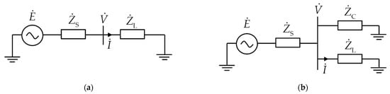
Figure 1.
Single-line diagram of simple impedance model for power system impedance identification: (a) Model without the parallel load consideration; (b) model with the parallel load consideration.
There are two unknown variables in Equation (1) and in the case of known (measured) variables and (which mainly represent positive sequence voltage and current). If we assume and as unknown variables, it is necessary to have almost two different samples of and to find . Unfortunately, and do not have to be constant during a real measurement. Different authors present different methods to find from the set of measured and . There are 7 different methods for power system impedance evaluation described in the next Section 2.1, Section 2.2, Section 2.3, Section 2.4, Section 2.5, Section 2.6 and Section 2.7.
2.1. Method No. 1
Method No. 1 was presented in 1997 by Srinivasan, Lafond, and Jutras [11]. Their considerations were based on the concept of a simplified model of the power system, according to Figure 1a. Equations (1) and (2) are rewritten in Equations (3) and (4), which are then expressed by derivation of each quantity in time in the form of Equations (5) and (6):
Based on the consideration that the change of the network impedance, as well as the change of the voltage of the equivalent source, are not related to the change of the load impedance, i.e., that and , the authors expressed the following relationship for calculating the power system impedance by multiplying Equations (5) and (6) and adjusting [11]:
where
- is equal mean of variable ,
- is equal complex conjugate of variable ,
- is equal the mean of the product .
This method was applied for positive sequence power system impedance computation from positive sequence voltage and current samples in this paper.
2.2. Method No. 2
Method No. 2 was presented in 2007 by Timbus, Rodrigues, Teodorescu, and Ciobotaru [12]. This method was based on the detection of dq components of voltage and load current . Authors state that the resistance and reactance of power system impedance can be expressed for every two samples of dq components of both voltage and current as follows:
Voltage and current dq components of the n-th sample can be calculated from their αβ components as follows:
where represents a general reference rotating frame.
Because this method was applied to a set of RMS values and angles of voltages and currents measured during each period, the general reference rotating frame was set to 0 for each sample.
2.3. Method No. 3
Method No. 3 was presented in 2009 by Arefifar and Xu [13]. Authors described an analytical solution of the three-point method, which was based on the identification of three-time samples for which , , and are constant during the measurement. If we consider 0 angle of current and complex voltage at each sample according to this method is calculated as a function of , as follows [13]:
where
According to this method can be found as a real solution of the simple second-order equation:
Equation (11) has been derived based on the assumption that the system side parameters remain unchanged for three different system conditions, and if for any reason the system side parameters vary for the three points, (11) is meaningless and will not have any solution.
After calculating and can be calculating and only variables that meet the following rules will be statistically evaluated:
- and should always be positive,
- should have feasible values.
In this paper, we consider feasible values for 110 kV voltage level and for 22 kV voltage level. We used this method for our analysis—even the author’s state in [13] that this three-point method was very sensitive to noise and transients in voltage and current measurement, and they recommended to extend the three-point method by including six or more measurement points through least square fitting.
2.4. Method No. 4
Method No. 4 was presented in 2010 by Bahadornejad and Nair [15] to estimate power system (Thevenin) impedance based on voltage and current changes measurement through on-load tap changer action of the power transformer. Although this method has been proposed to estimate power system impedance base on voltage and current changes measurement through on-load tap changer action, it brings an interesting statistical approach for power system impedance determination even for cases of large rapid current step changes. After modification of assumption of more than one tap action to more than one rapid current step change, we get for k-rapid current changes:
If we consider no correlation between load impedance changes and equivalent voltage source changes, i.e., , then:
Equation (13) was used to positive sequence power system impedance evaluation based on 2500 samples of largest RMS current changes, where is positive sequence voltage change in case of n-th positive sequence current change at place of load connection, is n-th positive sequence current change of load and is the is positive sequence load impedance change in case of n-th current change.
2.5. Method No. 5
Method No. 5 was presented in 2010 by Kanálik and Kolcun [16]. This method was very simple and was based only on the statistical evaluation of Equation (14) for positive sequence voltage and current changes:
The power system impedance was determined as a median of a set of values given by Equation (14). There was no recommendation for the minimum or the maximum number of samples to include in the statistical evaluation of Equation (14) in [16], but in the case of 10,000 samples, the best result for 2500 samples of largest RMS current changes was achieved. In the case of this paper, 2500 samples of the largest RMS current changes from 10,000 of total samples have been taken into account for power system impedance determination according to Equation (14). In addition, only samples, the following rules were taken into account for the median of a set of values evaluation:
- and should always be positive,
- should have feasible values.
In this paper, we consider feasible values for 110 kV voltage level and for 22 kV voltage level.
2.6. Method No. 6
Method No. 6 was presented in 2014 by Eidson, Geiger, and Halpin [17]. This method was based on the negative sequence voltage and current changes. This method was based on the assumption that the negative sequence component of the power system impedance equals its positive sequence component. The equivalent power system impedance, according to this assumption, can be found as [17]:
By separating the real and imaginary parts, the above equation can be written in the following matrix notation [17]:
where
The evaluation of and was provided as the median of a set of values given by Equation (16) for 2500 samples of largest positive sequence RMS current changes (for same samples as in methods No. 1, 2, 4, and 5).
2.7. Method No. 7
Method No. 7 was presented in 2019 by Wang, Xu, and Yong [18]. This method was based on the determination of , which was the power system impedance, including changes, i.e., . According to [18] can be found as follows:
The value represents the 95 percentile of possible equivalent voltage source variation without the effect of load impedance variation. It can be found from samples of meeting the condition:
where is the positive sequence load impedance and represents the measurement samples.
Power system evaluation, according to Equation (17), after the determination is then provided only for samples meeting the condition:
where ε is the acceptable error. In this paper, ε was selected as 15%, which, according to [18], means the error caused by the system variation is expected to be smaller than 15% with 95% possibility.
This method was applied for all samples of positive sequence voltage and current variations in this paper.
3. Application of Power System Estimation Methods on Simulated and Real Data
As mentioned above, the determination (estimation) of the power system impedance in real conditions, from real measurements of voltage and current changes at load, was based on the statistical evaluation of a larger amount of data in individual methods. The reason was the fact that the recorded voltage change at a particular load current change was to a greater or lesser extent (depending on the circumstances) also affected by a voltage change of the equivalent voltage source or by a natural change in the value of the equivalent power system impedance itself. The changes in the voltage of the equivalent voltage source or changes in the value of the equivalent power system impedance itself were not related to changes in the impedance of the measured load.
Due to the different approaches to determining the power system impedance within the individual methods described above, the outputs of these methods were compared with the known value of the power system impedance by a simple simulation test, the results of which are given in Section 3.1. Subsequently, the individual methods were applied to determine the power system impedance in the case of three real measurements. The results of power system impedance calculations in the case of real measurements are described in Section 3.2.
3.1. Simple Simulation Test
Testing of individual methods was performed using 2 simple power system models shown in Figure 1 created by MATLAB script. In the case of both models, the constant power system impedance = (0.5 + j4) Ω was considered. Within the power system model according to Figure 1a, the line-to-line voltage value of the equivalent voltage source changed randomly in the interval of 118 kV ± 0.1 kV, and the load impedance changed randomly in the interval of (300ej23.1° ± 12) Ω (only resistive part) within the 1st quarter simulated data and in the interval (300ej23.1° ± <−70; 9>) Ω (only resistive part) within the remaining three-quarters of the simulated data. In the case of the network model, according to Figure 1b, the line-to-line voltage of the equivalent voltage source and load impedance changed randomly at the same intervals as in Case 1 (a), but in addition, the parallel load impedance also changed randomly in the interval of (500ej18.2° ± 12) Ω. The total number of samples generated in each simulation was 1e4.
Figure 2, Figure 3 and Figure 4 show the time courses of the RMS voltage, the load impedance, as well as the RMS current of load in the case of a simulation carried out using a model without considering a parallel load (according to Figure 1a). Figure 2 shows the variation of the RMS voltage of the voltage source and of the voltage at the load. From the 2500th sample, there was a more pronounced variation in the load impedance (see Figure 3), which was reflected in an increase in the variation of the RMS voltage V.
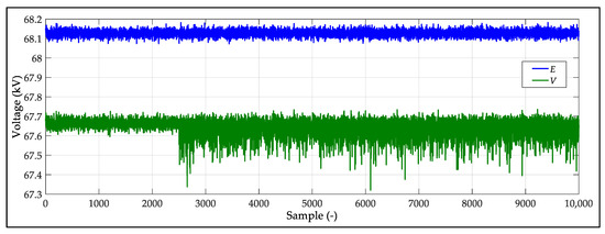
Figure 2.
Time course of root mean square (RMS) line-to-neutral voltage of the equivalent source and at load in the case of the model without the parallel load consideration.
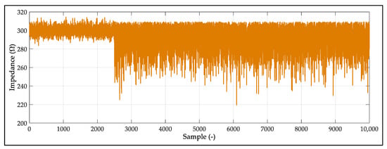
Figure 3.
Time course of load impedance magnitude in the case of the model without the parallel load consideration.
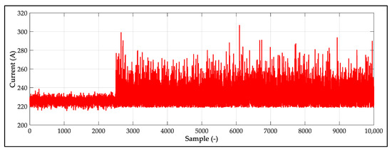
Figure 4.
Time course of RMS current of load in the case of the model without the parallel load consideration.
Table 1 shows the results of the evaluation of the power system impedance calculation using the individual methods applied by MATLAB script to the data shown in Figure 2, Figure 3 and Figure 4. Among all considered the methods described in Section 2, method No. 3 and method No. 6 were not applied for this analysis. In the case of method No. 3, the simulated data reached unrealistic results, probably due to the insufficient number of 3 consecutive samples with a constant value of load impedance. Determination of the power system impedance in the case of method No. 6 was based on analyzing the change in the negative sequence of the voltage and current, but the simulated data representing voltage and current changed only in a positive sequence. Calculation of the power system impedance using methods No. 1 to 5 was realized on the basis of the selection of 2500 samples with the largest current change. Only 1515 samples from selected 2500 samples met the criteria of the required impedance ( and ) in the case of method No. 5. In the case of method No. 7, all simulated samples were included in the calculation, but only 9 samples met the specified calculation criteria ( and ). As can be seen from the results in Table 1, all the methods tested led to the determination of the power system impedance (not only the size but also the ratio) with very good accuracy. The most accurate value of the power system impedance (set to value = (0.5 + j4) Ω) from the evaluated data was determined by method No. 1, and the least accurate value was determined using method No. 7 (however, due to the final number of samples (9) entering the calculation, the accuracy of the resulting value was excellent).

Table 1.
Statistical evaluation of power system impedance evaluation by application of particular methods on data simulated by the model without the parallel load consideration.
Figure 5, Figure 6 and Figure 7 show the time courses of the RMS voltage, the load impedance as well as the RMS current of load in the case of a simulation carried out using a model considering a parallel load (according to Figure 1b). Figure 5 shows the variation of the RMS voltage of the voltage source as well as of the voltage at the load. In addition, in this case, there was a more significant fluctuation of the load impedance from the sample of 2500 (see Figure 6), which was reflected in an increase in the fluctuation of the RMS voltage .
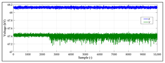
Figure 5.
Time course of RMS line-to-neutral voltage of the equivalent source and at load in case of the model with the parallel load consideration.
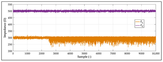
Figure 6.
Time course of load impedance magnitude in case of the model with the parallel load consideration.
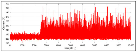
Figure 7.
Time course of RMS current of load in case of the model with the parallel load consideration.
Table 2 shows the results of the evaluation of the power system impedance calculation using the individual methods applied to the data shown in Figure 5, Figure 6 and Figure 7. Among all the considered methods described in Section 2, also in this case method No. 3 and method No. 6 were not applied for this analysis due to the same reasons as in the previous case. Calculation of the power system impedance using methods No. 1 to 5 was realized on the basis of the selection of 2500 samples with the largest current change. Only 1458 samples from selected 2500 samples met the criteria of the required impedance ( and ) in the case of method No. 5. In the case of method No. 7, all simulated samples were included in the calculation, but only 11 samples met the specified calculation criteria ( and ). As can be seen from the results in Table 2, even in this case all the methods tested led to the determination of the power system impedance (not only the size but also the ratio) with very good accuracy (the value of power system impedance was set to = (0.5 + j4) Ω in the model). The most accurate value of the power system impedance from the evaluated data was determined by method No. 1, 2, 4, and the least accurate value was determined using method No. 7 (however, due to the final number of samples (11) entering the calculation, the accuracy of the resulting value was excellent also in this case).
Table 2.
Statistical evaluation of power system impedance evaluation by application of particular methods on data simulated by the model with the parallel load consideration.
3.2. Real Measurement Test
The application of individual methods for determining the power system impedance from real measured data was realized using 3 measurements of the time course of the RMS value and the angle of voltage and current in 110 kV, and at a 22 kV substation supplying a steel mill with an electric arc furnace (EAF) operation.
In the case of the first 2 measurements, it was the same measuring point (supplying the Steel mill 1), but under different conditions in the 110 kV distribution grid configuration. A single-line diagram for measurement No. 1 and 2 is shown in Figure 8a. Based on information from the distribution system operator, the level of short-circuit power within the considered 110 kV substation, depending on the configuration of the power system and the operation of the sources, can range from 1000 MVA to 3700 MVA. According to the assumptions of the distribution system operator, the configuration of the power system at the time of measurement No. 1 led to the value of short-circuit power in the 110 kV substation to the level from 2800 MVA to 3200 MVA, which represents the value of the power system impedance in the interval 4.2 Ω to 4.8 Ω. Power system configuration at the time of measurement No. 2 led, according to the assumptions of the distribution system operator, to the value of short-circuit power in the 110 kV substation to the level from 1600 MVA to 1900 MVA, which represents the value of the network impedance in the interval 7.0 Ω to 8.3 Ω.
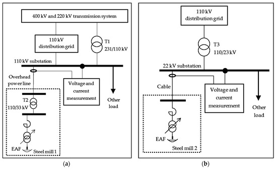
Figure 8.
Single-line diagram of real measurement test realization: (a) Measurement No. 1 and No. 2 in 110 kV substation supplying Steel mill 1; (b) measurement No. 3 in 22 kV substation supplying Steel mill 2.
In the case of the 3rd measurement, it was a measuring point in the 22 kV substation, from which Steel mill 2, also with the operation of the arc furnace, was supplied. A single-line diagram for measurement No. 3 is shown in Figure 8b. The 22 kV substation was supplied from the 110 kV distribution system only through one 110/23 kV transformer with a nominal power of 16 MVA, a short-circuit voltage of 10.7%, and nominal load losses of 77.5 W. The maximum value of short-circuit power on the 22 kV busbar of this substation was guaranteed at the level of 148 MVA, which represents a power system impedance of approximately 3.6 Ω. Since the positive sequence impedance of the transformer T3 represents a value of 3.48 Ω (according to Section 6.3 of IEC 60909-0: 2016), the measured value of the power system impedance should not fall below this value.
In the case of all 3 measurements, 10 min recordings of RMS values and angles of voltages and currents of the fundamental frequency (50 Hz) with a recording interval of 1 period (0.02 s) were performed. The total number of recorded and thus evaluated data was 30,000 samples for each measurement.
Figure 9 and Figure 10 show the time courses of the RMS values of voltages and currents, or angles of voltages and currents in all 3 phases measured in measurement No. 1. Within the first 240 samples, it was possible to observe the magnitude of the voltage as well as the level of its fluctuation without the operation of the EAF (in Figure 9). Subsequently, it was possible to observe the effect of the RMS current variation on the variation of the RMS voltage during the operation of the EAF.
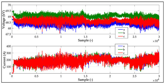
Figure 9.
Time course of RMS voltage and current measured during measurement No. 1.
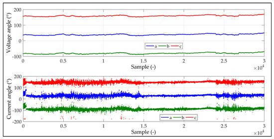
Figure 10.
Time course of angles of voltage and current measured during measurement No 1.
Figure 11 and Figure 12 show the time courses of the RMS values of voltages and currents, or angles of voltages and currents in all 3 phases measured in measurement No. 2. In this case, it was possible to observe the magnitude of the voltage as well as the level of its fluctuation without the operation of the EAF within 4 significant intervals (see Figure 11). In addition, it can be seen in Figure 11 the effect of fluctuations in RMS current on fluctuations in RMS voltage during EAF operation.
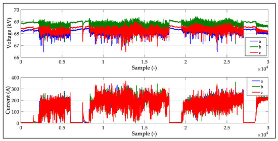
Figure 11.
Time course of RMS voltage and current measured during measurement No. 2.
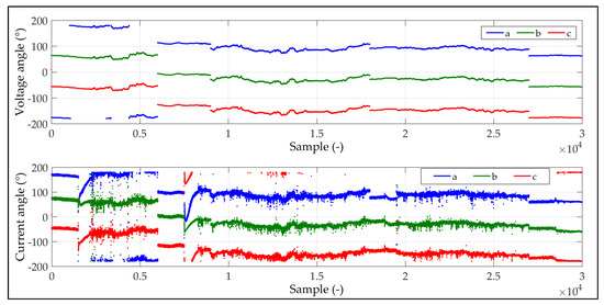
Figure 12.
Time course of angles of voltage and current measured during measurement No. 2.
Figure 13 and Figure 14 show the time courses of the RMS values of voltages and currents, or angles of voltages and currents in all 3 phases measured in measurement No. 3. In addition, in this case, it was possible to observe the magnitude of the voltage as well as the level of its fluctuation without the operation of the arc furnace within 4 more significant intervals (see Figure 13), as well as the effect of fluctuations in RMS current on fluctuations in RMS voltage, can also be observed.
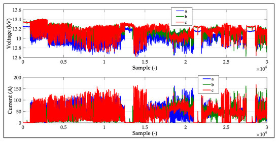
Figure 13.
Time course of RMS voltage and current measured during measurement No. 3.
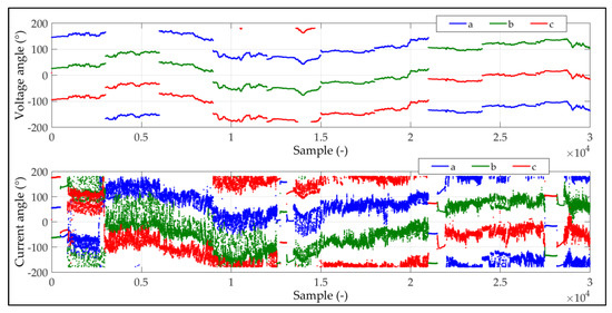
Figure 14.
Time course of angles of voltage and current measured during measurement No. 3.
The evaluation of the power system impedance was performed using all 7 considered methods from the measured data. Methods No. 3 and No. 7 were designed to consider only data meeting the assumptions of these methods from the whole data set. In the case of other methods, only samples corresponding to 2500 of the largest step changes in the RMS value of the positive sequence current were considered for the power system impedance evaluation. Because method No. 6 was designed to evaluate power system impedance based on step changes of the negative sequence voltages and currents, we applied this method for 2 different sets of 2500 samples. The 1st set of 2500 samples was the same as for the other methods (i.e., corresponding to 2500 of the largest step changes in the RMS value of the positive sequence current), and we labeled this approach as 6a. The 2nd set of 2500 samples was corresponding to 2500 of the largest step changes in the RMS value of the negative sequence current, and we labeled this approach as 6b. Table 3 shows the final numbers of samples from which the power system impedance calculations were performed by individual methods in the case of measurements No. 1 to 3. Subsequently, Table 4, Table 5 and Table 6 show the results of the calculations of resistance (RS), reactance (XS), and the magnitude of the total power system impedance (ZS) calculated for each measurement using the individual methods. Asterisks (*) in these tables indicate values that did not meet the assumptions or represent an unrealistic value.
Table 3.
The number of samples used in power system impedance evaluation by application of particular methods on real measured data.
Table 4.
Statistical evaluation of resistance () in ohms of power system impedance by application of particular methods on real measured data.
Table 5.
Statistical evaluation of reactance () in ohms of power system impedance by application of particular methods on real measured data.
Table 6.
Statistical evaluation of the magnitude of power system impedance () in ohms by application of particular methods on real measured data.
The results of the power system impedance determined by individual methods in the case of 3 sets of real measured data presented in this article show their greater ambiguity, as it was in the case of their application to simulated data (described in Section 1).
In the case of measurement No. 1, it was possible to observe the results of the calculation within the expected interval (4.2 Ω to 4.8 Ω) within methods No. 1 to 5. However, even in the case of methods No. 6 and 7, a realistic value was determined. A possible reason for a larger deviation of the calculated value of the power system impedance from other methods in the case of method No. 6 was the fact that this method was based on the assessment of the change in the negative sequence of voltage and current, while the samples selected for analysis has been selected on the basis of the largest positive sequence current changes. In the case of method No. 7, it met the specified calculation criteria ( and ) with only 19 samples, which was relatively small out of the total number of 30,000 samples.
Measurement No. 2 pointed out a more fundamental problem in the application of methods No. 3 and 4 for a given data set. In these 2 cases, too high values of the power system impedance, and in the case of method No. 4, negative power system reactance values were calculated. Other methods led to the calculation of the realistic value of the power system impedance, although the results of the calculation obtained using methods No. 2 and 6 were more pronounced than the expected value.
Measurement No. 3 was realized in a substation, within which it was clear that the magnitude of the power system impedance could not be less than 3.48 Ω and at the same time, it was not assumed that the value of 4.8 Ω should not be exceeded. In this case, the expected results were obtained using methods No. 1, 5, and 6, although in the case of method No. 1, a negative network resistance value was determined. Since this value was close to 0, it can be assumed that this was a certain statistical deviation within the selected data set. Although impedance values obtained by methods No. 3 and 7 represented a realistic value, they moved more significantly from the expected result. Methods No. 2 and 4 completely failed in this case.
Among the analyzed methods, methods No. 1 and No. 5 seemed to be the most suitable for power system impedance estimation based on fast voltage and current changes measurements. Nevertheless, based on the obtained results, it is not possible to say unequivocally that these 2 methods are more suitable or less suitable for determining the power system impedance within a wide range of measured data. In this context, it should be emphasized that the individual methods have been applied to a specific type of data measured during the operation of EAF. Methods No. 3 and 7 were designed to determine the power system impedance within the standard steady-state operation, within which, for example, it would not be possible to apply method No 5.
4. Discussion
A very important question in the case of the power system (Thevenin) impedance finding is what kind of impedance we are interested in and the reason for this impedance identification. Different size of power system impedance can be evaluated from the rapid voltage and current change, where subtransient reactances of synchronous machines or reaction of induction motors are included, and a different size of power system impedance can be evaluated from the comparison of steady-state voltage and current changes, where no subtransient reactances of synchronous machines or reaction of induction motors are included. In addition, voltage regulation can also affect the result. If the interests of power system impedance deals with the power system weakness or with the initial short-circuit current (power) identification, rapid changes of voltages and currents should be used for the analysis. For this reason, the success of methods for power system impedance identification depends on the size of the measured current change in comparison to the current change of other currents (loads) affected measured voltage change. Voltage changes recorded due to current changes in all three sets of data presented in this paper are large enough to find positive sequence power system impedance representing to the behavior of the power system in case of rapid current changes. On the other hand, the operation of EAF leads to a change in the current more than once per cycle. Due to EAF operation (mainly at the beginning of each duty cycle), changes in load impedance occur a few times per cycle and are not symmetrical. This fact causes very large current waveform deformation, i.e., 50 Hz RMS voltage and current changes can be skewed.
Based on the above-presented results and facts, it is possible to state the following properties of particular methods analyzed in this paper:
- Method No. 1 seems to be suitable for power system impedance estimation based on rapid voltage and current changes. There is no selection of data meeting any criteria in this method, thus some noise in the data can affect the result.
- In the case of method No. 2, the inaccurate results can be obtained in the case of an unbalanced three-phase system, which leads to oscillation of α and β components even in steady-state, i.e., without the change in load impedance or current.
- Method No. 3 was not suitable for power system impedance estimation based on rapid voltage and current changes. In addition, the authors of this method recommend extending the solution based on a three-point to at least a six-point solution [13].
- Nevertheless, method No. 4 was very successful in the case of a simulation test of power system impedance identification; it totally failed in the case of real measured data application. The problem of this method could be solved in the future by proposing additional criteria for the selection of samples entering into the calculation. The selection of suitable samples in this case obviously cannot be based only on the magnitude of RMS current the step change. Even a small number of large but inadequate changes in load impedance (), as well as in RMS voltage () corresponding to selected current step changes, can significantly affect the overall result. As an example of increasing the accuracy of this method, we present the fact that after removing 5% of samples with the highest values , , and , , the following three impedance values were obtained for individual measurements using this method:
- ∘
- = (1.098 + j4.307) Ω in the case of measurement No. 1,
- ∘
- = (1.365 + j7.247) Ω in the case of measurement No. 2,
- ∘
- = (1.249 + j1.652) Ω in the case of measurement No. 3,
These values came significantly closer to the expected values. The emphasis on determining the criteria for selecting suitable samples can contribute to a significant extension of the applicability of this method in the future.
- Although method No. 5 is very simple, this method seems to be very strong for purposes of power system impedance estimation based on rapid voltage and current changes. In the case of this method, it is necessary for the future to focus on determining the criteria for determining the minimum value of the RMS current step change for the selection of suitable samples of data. The recent criterion for suitable data selection does not analyze the extent of the effect of RMS current step change on RMS voltage step change. If there were RMS voltage step changes at the level of RMS voltage step changes without measured current (or similar to RMS current step change close to zero) in the case of selected RMS current step changes, the results of the power system impedance calculation would be very inaccurate. The analysis of the variation of the RMS voltage in a given node without the influence of the measured load seems to be key for estimating the applicability of this method in specific conditions.
- In the case of method No. 6, significantly lower values of power system impedance have been achieved against other methods. This fact was independent of whether the data set evaluated by this method was filtered on the basis of the 2500 largest RMS changes in the positive sequence current or on the basis of the 2500 largest RMS changes in the negative sequence current.
- Method No. 7 is a perspective method, but even in the case of 10,000 samples in three different measurements, there was a lack of data meeting the given criteria.
One of the possible way to check the accuracy of evaluated power system impedance is also to calculate the voltage of the Thevenin equivalent voltage source (see Figure 1a)) and consequently to compute the voltage at the measured point in the steady-state, i.e., when no rapid voltage and/or current changes occur.
Further research in this field could be focused on a better description of the minimal size of necessary current changes in connection to background voltage changes, as well as on the possibility of improving the criteria for selecting suitable samples for the purpose of calculating the power system impedance using the methods described above.
5. Conclusions
The aim of this article was to present the results of the power system impedance calculation realized by the analysis of real measured data through seven different methods. The specificity of the presented results meets the fact that the evaluated data were measured in HV and MV substations supplying steel mills with the operation of EAF. In the case of this type of load, there are very fast and large step changes in the current, which is naturally reflected in the fast and significant voltage changes at the measured busbar. Despite significant changes in voltages and currents during the operation of this type of load, determining the equivalent power system impedance is not an easy task. The reason is the fact that the basic principle of determining the power system impedance is based on the identification of voltage response to a current change at the measuring point. However, the voltage at the measuring point is not constant even in the case of no current changes. If the fact that the value of the equivalent power system impedance may not be constant during the measurement is added to the natural fluctuation of the background voltage, the estimation of the equivalent power system impedance becomes more complicated. The authors of each of the seven methods considered in this paper tried to deal with this situation in different ways.
In the case of method No. 1, the authors derived the relationships between the power system impedance and the mean complex vectors of voltages and currents (in our case, of the positive sequence component). However, the authors of this method did not specify the criteria for the selection of suitable samples to be included in the calculation. Due to the fact that the calculation is performed by determining the median of complex voltage and current vectors from a larger amount of data, a smaller number of samples that do not meet the assumptions of this method will not significantly affect the result of the calculation. On the other hand, in the case of a higher degree of inconsistency of the samples entering the calculation, these samples may have a significant effect on the result of the calculation.
In the case of method No. 2, the authors derived equations for the resistance and reactance of the equivalent power system impedance using the αβ transformation of three-phase voltages and currents to determine the magnitudes of the voltage and current components in the dq system. This approach circumvents the transformation of a three-phase system into a symmetrical components system while bringing relatively simple equations. On the other hand, even in the case of this method, the determination of criteria for the selection of suitable samples entering the calculation is absent. In contrast to the problem of errors due to the existence of natural voltage fluctuations in the measured node, its sensitivity to the level of voltage and/or current unbalance may be a disadvantage of this method. The transformation of the three-phase system of voltages as well as currents into the αβ system is realized through instantaneous values of voltages and currents. In the case of an unbalanced three-phase system, the α and β components oscillate during one period (20 ms), even in a steady-state, when the RMS values of voltages and currents in the positive and negative system are constant. In addition, if this methodology is used in the analysis of three-phase voltages and currents, which even change their amplitude or angle during the measurement, the result of the calculation will also depend on the time when voltage and current changes occur. Therefore, the use of this method is limited mainly to use it in three-phase systems with a minimum level of unbalance.
Authors of method No. 3 focused on solving the problem of natural voltage fluctuations or power system impedance fluctuations in the measured node by deriving equations based on not only two but up to three consecutive samples of measured data. The advantage of this method is its automatic selection of inconsistent samples. As the authors of this method state themselves in [13], the use of the three-point method is relatively inaccurate, despite the automatic selection of suitable samples, and they recommend the derivation of the power system impedance calculation based on a six-point approach.
The advantage of method No. 4 is that the degree of the load impedance change at a given voltage or current change is also taken into account in the calculation of the power system impedance. This method was primarily designed to determine the power system impedance from the measurement of voltage and current changes in the case of the power transformer’s tap changing. Its use to analyze data recorded in the case of rapid and significant load current changes (such as during EAF operation) requires further research on the criteria for suitable data sample selection determination (for more details, see the Discussion section in this paper).
The advantage of method No. 5 is its simplicity and clarity. This method solves the problem of fluctuations in network voltage as well as in power system impedance only at the level of statistical evaluation of a sufficient amount of data. The results presented in this paper suggest its excellent applicability to data measured on EAF type of loads. On the other hand, even in this case, it is possible to focus further research on the creation of criteria for the selection of suitable samples entering the statistical evaluation.
In the case of method No. 6, the authors tried to derive equations for the calculation of resistance and reactance of the power system based on the measurement of changes in complex vectors of voltages and currents in the negative sequence system. Even in this case, the authors did not define any further criteria for the selection of suitable samples to be included in the calculation. The use of this method is especially suitable in networks with a large level of unbalance or with unbalanced load changes. When using this method to measure impedance in conditions where the dominant step changes of voltages and currents take place in the positive sequence system, it seems more advantageous to modify this method to analyze the voltages and currents in the positive sequence system.
Method No. 7 represents a very complex method. During its development, the authors dealt with a large extent, with the influence of natural voltage fluctuations in the power system or even the influence of fluctuations in the power system impedance itself. Determination of natural voltage fluctuations is based on the identification of samples with less than 0.1% change in load impedance (measured load). Although this method shows an excellent accuracy in data analysis with slower and not so significant changes in current and voltage, its application to data measured at load with very fast and large current changes appears to be unsuitable.
In future research, in addition to the analysis of the determination of sampling criteria within the individual methods, it would be appropriate to address the issue of identifying natural voltage fluctuations in a given node without the influence of the measured load. The correctness of the determination of the equivalent power system impedance realized on the basis of data measured during changes of voltages and currents could in the future be assessed by additional calculation of the magnitude of the voltage on the measured busbar. This calculation could be performed on the principle of the difference between the estimated voltage of the equivalent power system source and the voltage drop given by the current flowing through the estimated power system impedance during a steady-state operation.
Author Contributions
Conceptualization, M.K. and A.M.; methodology, M.K. and A.K.; software, M.K. and A.K.; validation, Ľ.B.; formal analysis, M.K. and Ľ.B.; investigation, A.M.; resources, A.M.; writing—original draft preparation, M.K.; writing—review and editing, M.K. and A.M.; visualization, A.M.; supervision, M.K. All authors have read and agreed to the published version of the manuscript.
Funding
This research received no external funding.
Institutional Review Board Statement
Not applicable.
Informed Consent Statement
Not applicable.
Data Availability Statement
Not applicable.
Conflicts of Interest
The authors declare no conflict of interest.
References
- Mou, X.; Li, W.; Li, Z. A preliminary study on the Thevenin equivalent impedance for power systems monitoring. In Proceedings of the 4th International Conference on Electric Utility Deregulation and Restructuring and Power Technologies (DRPT), Weihai, Shandong, China, 6–9 July 2011. [Google Scholar]
- Sun, T.; Li, Z.; Rong, S.; Lu, J.; Li, W. Effect of load change on the Thevenin equivalent impedance of power system. Energies 2017, 10, 330. [Google Scholar] [CrossRef]
- Kataras, B.; Jóhannsson, H.; Nielsen, A. Voltage stability assessment accounting for non-linearity of Thévenin voltages. IET Gener. Transm. Distrib. 2020, 14, 3338–3345. [Google Scholar] [CrossRef]
- Dalali, M.; Karegar, H.K. Voltage instability prediction based on reactive power reserve of generating units and zone selection. IET Gener. Transm. Distrib. 2019, 13, 1432–1440. [Google Scholar] [CrossRef]
- Lee, Y.; Han, S. Real-time voltage stability assessment method for the Korean power system based on estimation of Thévenin equivalent impedance. Appl. Sci. 2019, 9, 1671. [Google Scholar] [CrossRef]
- Su, H. An efficient approach for fast and accurate voltage stability margin computation in large power grids. Appl. Sci. 2016, 6, 335. [Google Scholar] [CrossRef]
- Chang, P.; Dai, J.; Tang, Y.; Yi, J.; Lin, W.; Yu, F. Research on analytical method of Thevenin equivalent parameters for power system considering wind power. In Proceedings of the 12th IEEE PES Asia-Pacific Power and Energy Engineering Conference (APPEEC), Nanjing, China, 20–23 September 2020. [Google Scholar]
- Duong, D.T.; Uhlen, K. Online voltage stability monitoring based on PMU measurements and system topology. In Proceedings of the 3rd International Conference on Electric Power and Energy Conversion Systems, Istanbul, Turkey, 2–4 October 2013. [Google Scholar]
- IEC 60909-0:2016. Short-Circuit Currents in Three-Phase a. c. Systems—Part 0: Calculation of Currents; CENELEC: Brussels, Belgium, 2016. [Google Scholar]
- Kolcun, M.; Kanálik, M.; Medveď, D.; Čonka, Z. Measuring of real value of short-circuit power in island operation condition. In Proceedings of the 16th International Scientific Conference on Electric Power Engineering (EPE), Kouty nad Desnou, Czech Republic, 20–22 May 2015. [Google Scholar]
- Srinivasan, K.; Lafond, C.; Jutras, R. Short-circuit current estimation from measurements of voltage and current during disturbances. IEEE Trans. Ind. Appl. 1997, 33, 1061–1064. [Google Scholar] [CrossRef]
- Timbus, A.; Rodriguez, P.; Teodorescu, R.; Ciobotaru, M. Line impedance estimation using active and reactive power variations. In Proceedings of the IEEE Power Electronics Specialists Conference, Orlando, FL, USA, 17–21 June 2007. [Google Scholar]
- Arefifar, S.; Xu, W. Online tracking of power system impedance parameters and field experiences. In Proceedings of the IEEE PES General meeting, Providence, RI, USA, 25–29 July 2010. [Google Scholar]
- Arefifar, S. Online Measurement and Monitoring of Power System Impedance and Load Model Parameters. Master’s Thesis, University of Alberta, Edmonton, AB, Canada, 2004. [Google Scholar]
- Bahadornejad, M.; Nair, N. System Thevenin impedance estimation through on-load tap changer action. In Proceedings of the 20th Australasian Universities Power Engineering Conference, Christchurch, New Zealand, 5–8 December 2010. [Google Scholar]
- Kanálik, M.; Kolcun, M. The principle of actual short-circuit power determination in different nodes of the power system. In Proceedings of the 7th International Scientific Symposium on Electrical Power Engineering (Elektroenergetika 2013), Stará Lesná, Slovakia, 18–20 September 2013. [Google Scholar]
- Eidson, B.; Geiger, D.; Halpin, M. Equivalent power system impedance estimation using voltage and current measurements. In Proceedings of the Clemson University Power Systems Conference, Clemson, SC, USA, 11–14 March 2014. [Google Scholar]
- Wang, Y.; Xu, W.; Yong, J. An adaptive threshold for robust system impedance estimation. IEEE Trans. Power Syst. 2019, 34, 3951–3953. [Google Scholar] [CrossRef]
- Tsai, S.; Wong, K. On-line estimation of thevenin equivalent with varying system states. In Proceedings of the IEEE Power and Energy Society General Meeting—Conversion and Delivery of Electrical Energy in the 21st Century, Pittsburgh, PA, USA, 20–24 July 2008. [Google Scholar]
- Alinezhad, B.; Karegar, H. On-line Thévenin impedance estimation based on PMU data and phase drift correction. IEEE Trans. Smart Grid 2018, 9, 1033–1042. [Google Scholar] [CrossRef]
- Abdelkader, S.; Morrow, D. Online Thévenin equivalent determination considering system side changes and measurement errors. IEEE Trans. Power Syst. 2015, 30, 2716–2725. [Google Scholar] [CrossRef]
- Wang, M.; Liu, B.; Deng, Z. An improved recursive assessment method of Thevenin equivalent parameters based on PMU measurement. In Proceedings of the IEEE Power Engineering and Automation Conference, Wuhan, China, 8–9 September 2011. [Google Scholar]
- Didehvar, S.; Chabanloo, R. Accurate estimating remote and equivalent impedance for adaptive one-ended fault location. Electr. Power Syst. Res. 2019, 170, 194–204. [Google Scholar] [CrossRef]
- Seo, H. New protection scheme in loop distribution system with distributed generation. Energies 2020, 13, 5897. [Google Scholar] [CrossRef]
- Staroszczyk, Z. A method for real-time, wide-band identification of the source impedance in power systems. IEEE Trans. Instrum. Meas. 2005, 54, 377–385. [Google Scholar] [CrossRef]
- Xie, J.; Feng, Y.; Krap, N. Network impedance measurements for three-phase high-voltage power systems. In Proceedings of the Asia-Pacific Power and Energy Engineering Conference, Chengdu, China, 28–31 March 2010. [Google Scholar]
- Nezhadi, M.; Hassanpour, H.; Zare, F. Grid impedance estimation using low power signal injection in noisy measurement condition based on wavelet denoising. In Proceedings of the 3rd Iranian Conference on Intelligent Systems and Signal Processing (ICSPIS), Shahrood, Iran, 20–21 December 2017. [Google Scholar]
- Mohammed, N.; Ciobotaru, M.; Town, G. Online parametric estimation of grid impedance under unbalanced grid conditions. Energies 2019, 12, 4752. [Google Scholar] [CrossRef]
- Suárez, J.; Gomes, H.; Filho, A.S.; Fernandes, D.; Costa, F. Grid impedance estimation for grid-tie inverters based on positive sequence estimator and morphological filter. Electr. Eng. 2020, 102, 1195–1205. [Google Scholar] [CrossRef]
Publisher’s Note: MDPI stays neutral with regard to jurisdictional claims in published maps and institutional affiliations. |
© 2020 by the authors. Licensee MDPI, Basel, Switzerland. This article is an open access article distributed under the terms and conditions of the Creative Commons Attribution (CC BY) license (http://creativecommons.org/licenses/by/4.0/).