New Second-Order Sliding Mode Control Design for Load Frequency Control of a Power System

 , ,
, ,
Abstract
1. Introduction
- The second-order sliding mode controller based on integral sliding surface is offered to ensure the shortening of the frequency’s transient response to avoid the overshoot.
- A new LMI technique is derived to guarantee the stability of whole system via Lyapunov theory.
- The simulation results show and clearly prove the usefulness, the effectiveness and the robustness of the proposed second order SMC approach against the various disturbances such as matched, mismatched uncertainties and load variations. In comparison, the performance of the proposed SOISMC is better than the previous control by using differential games method given in [10].
2. Mathematical Model of an Interconnected Multi-Area Power Network
3. A New Second Order Sliding Mode Load Frequency Control Design
3.1. Stability Analysis of the Multi-Area Power Network in Sliding Mode Dynamics
3.2. Load Frequency Controller Design
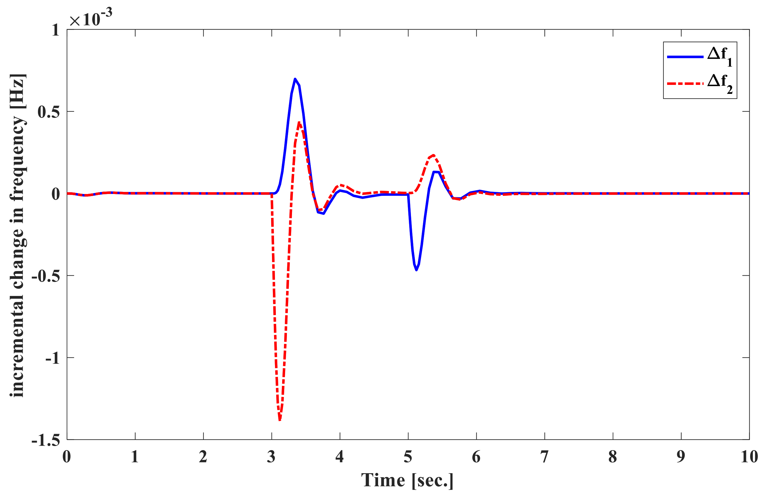
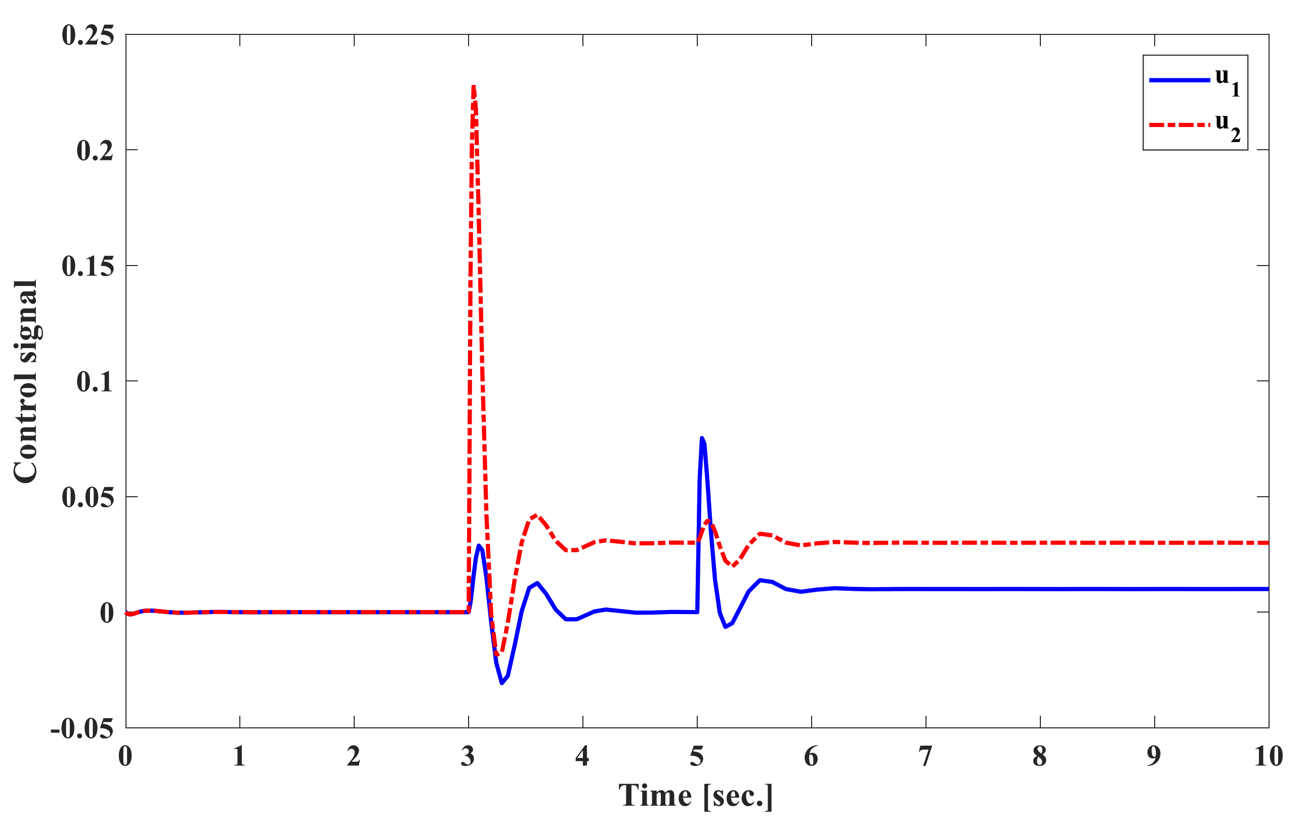
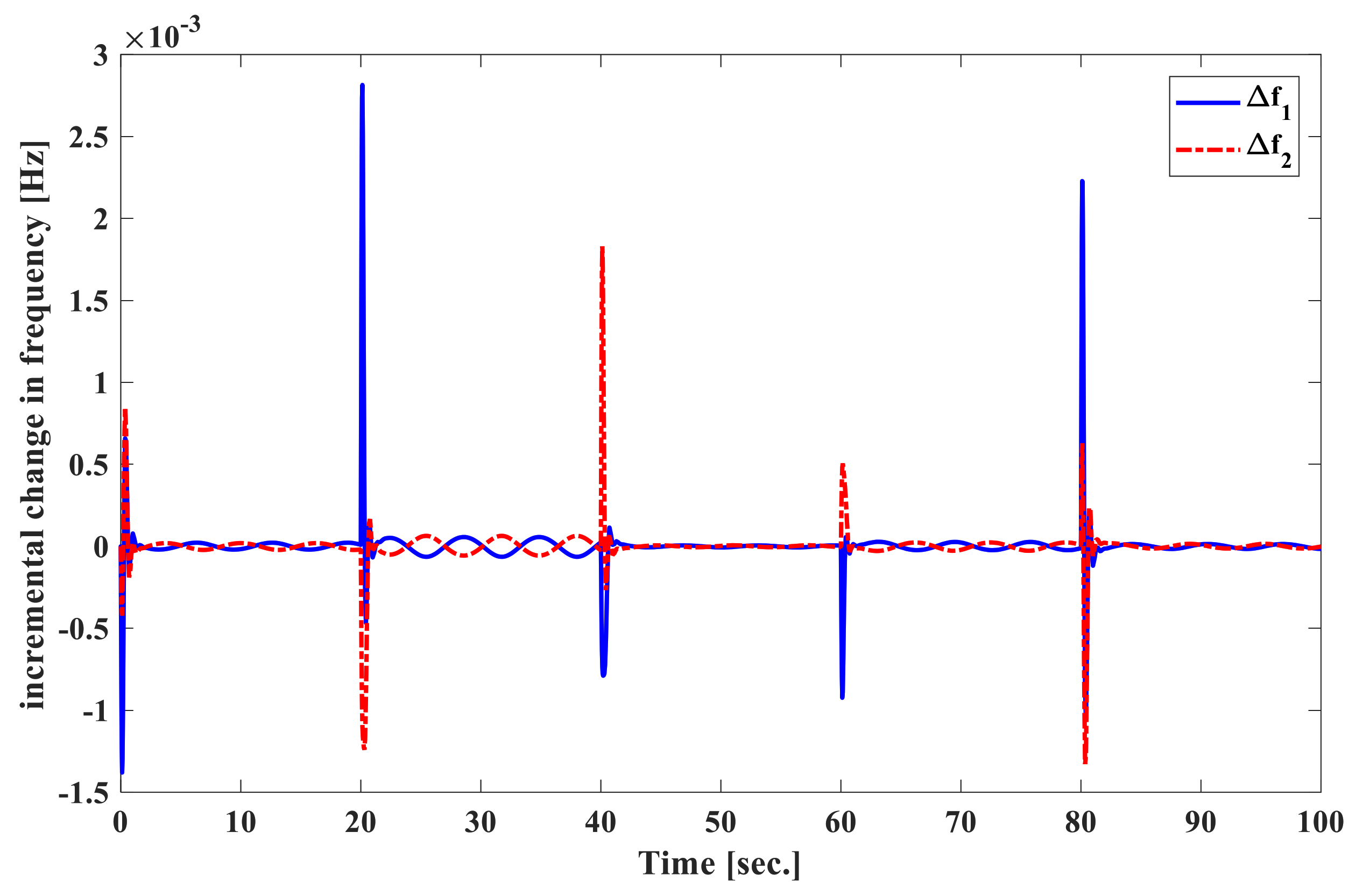
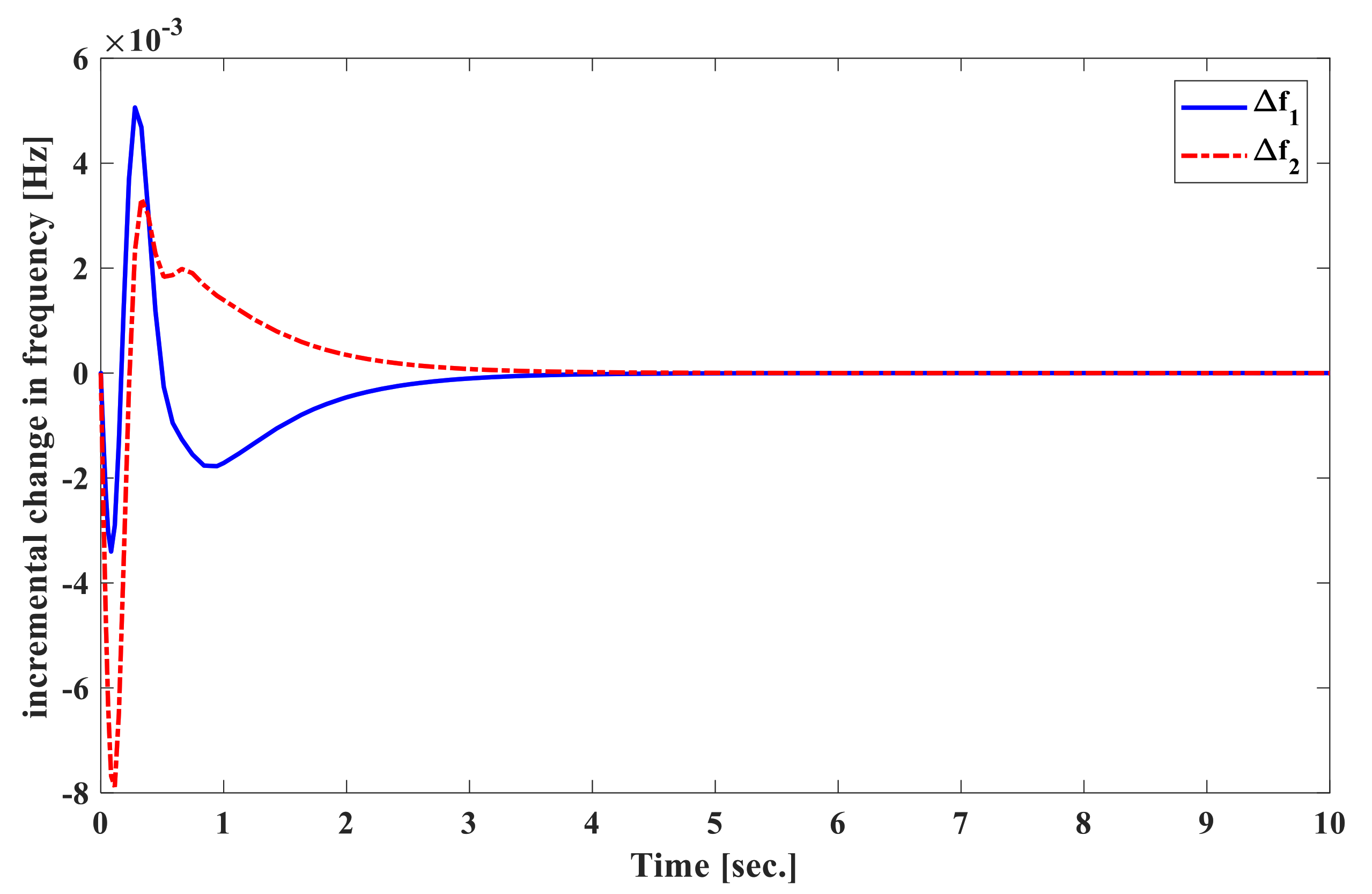
4. Simulation Results
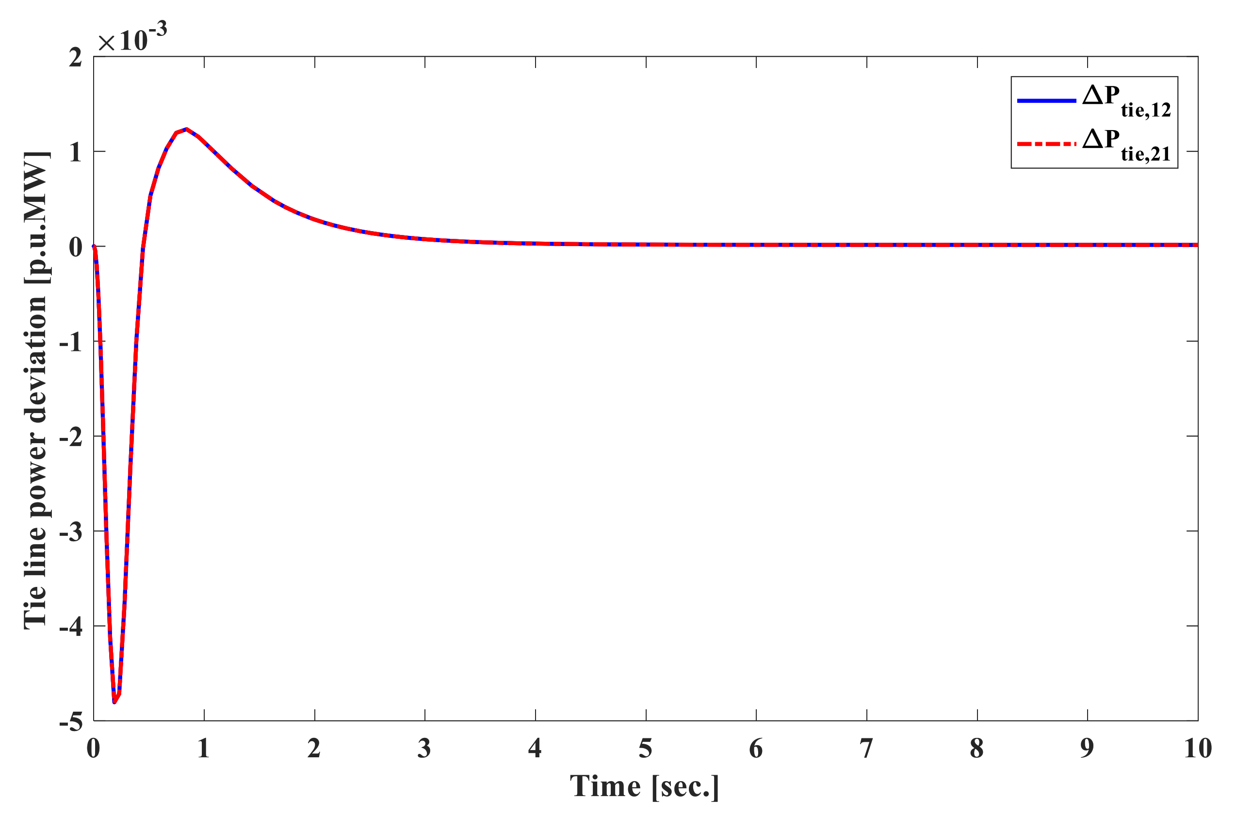
4.1. Simulation 1
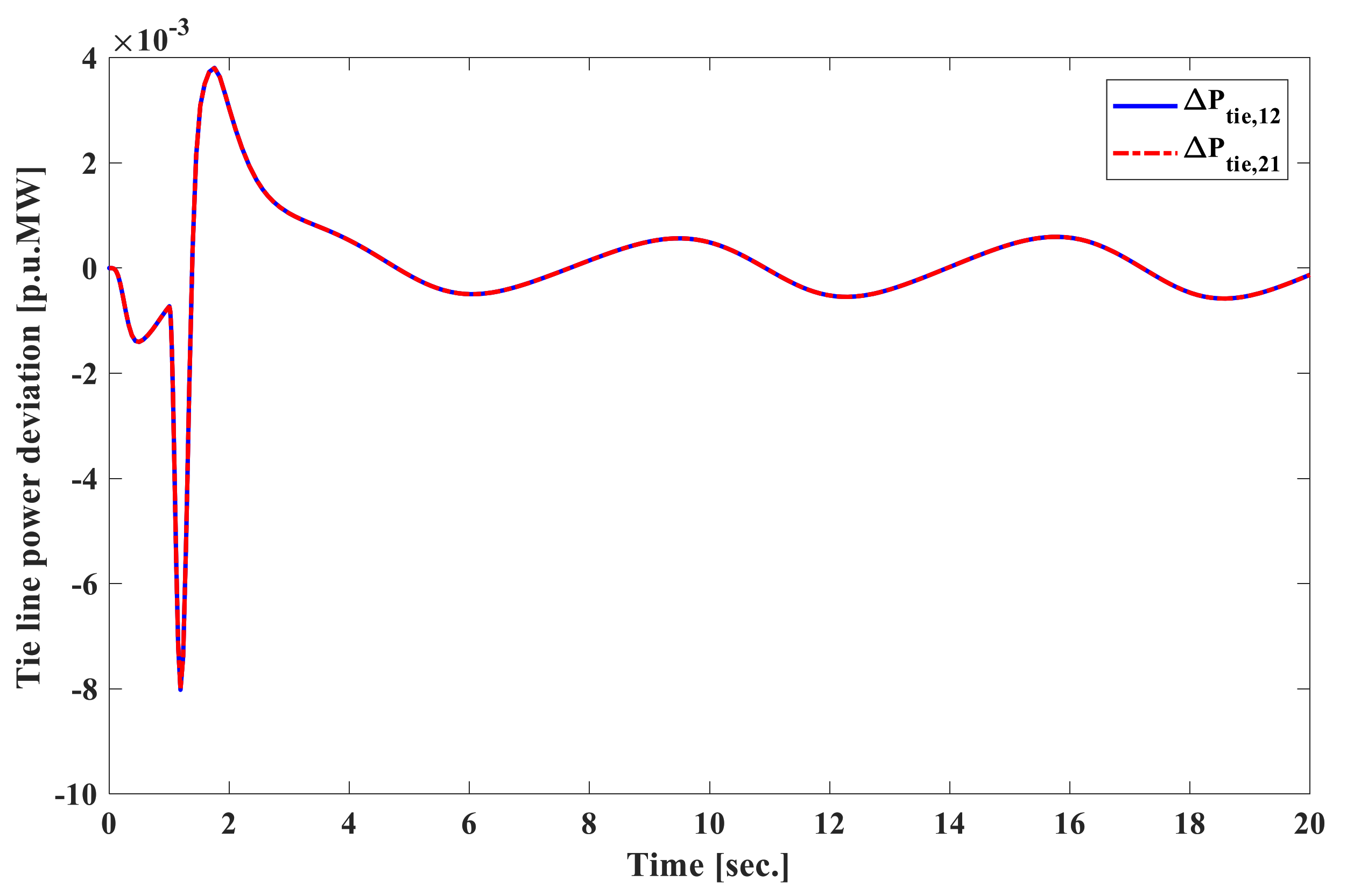
4.2. Simulation 2
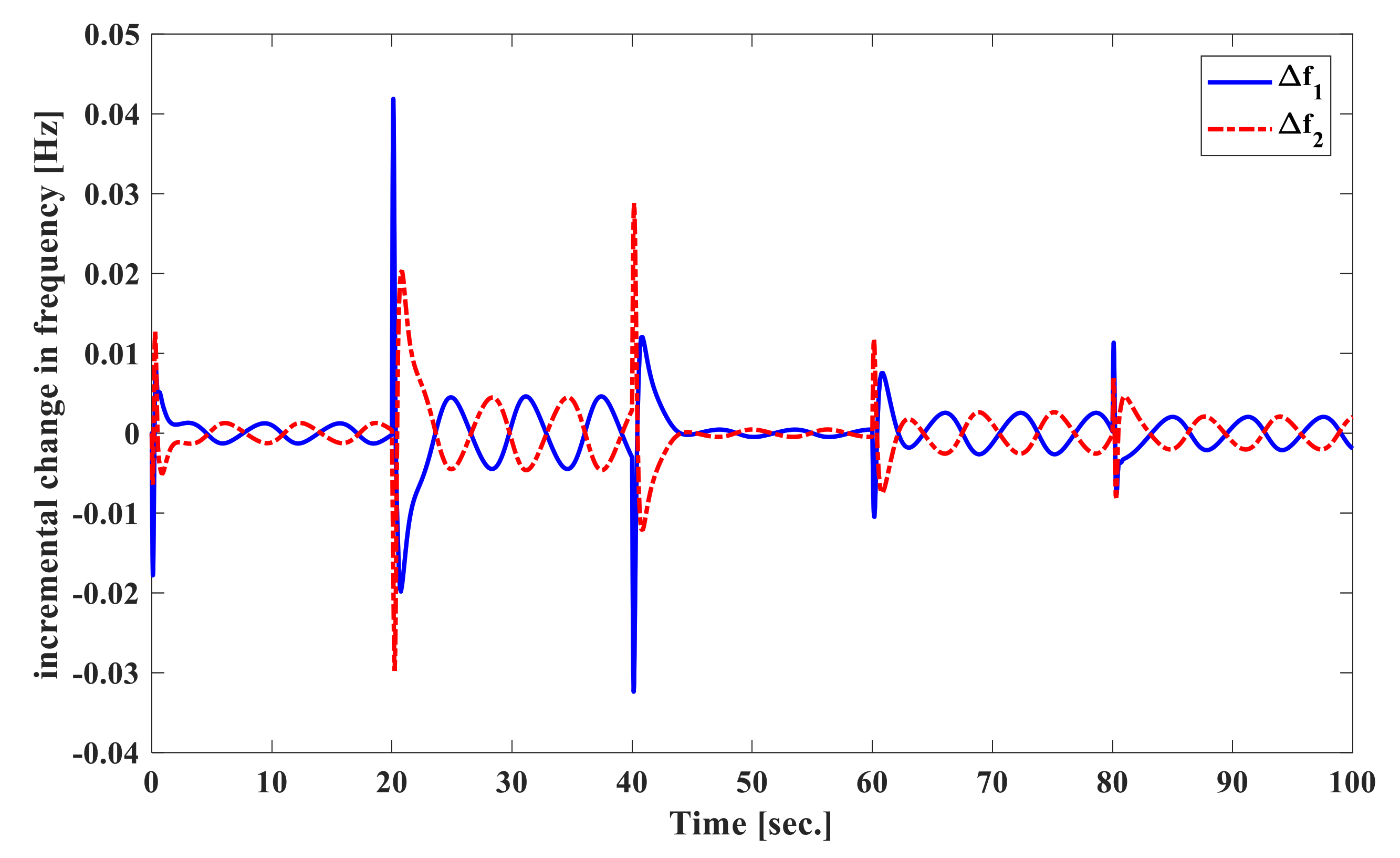
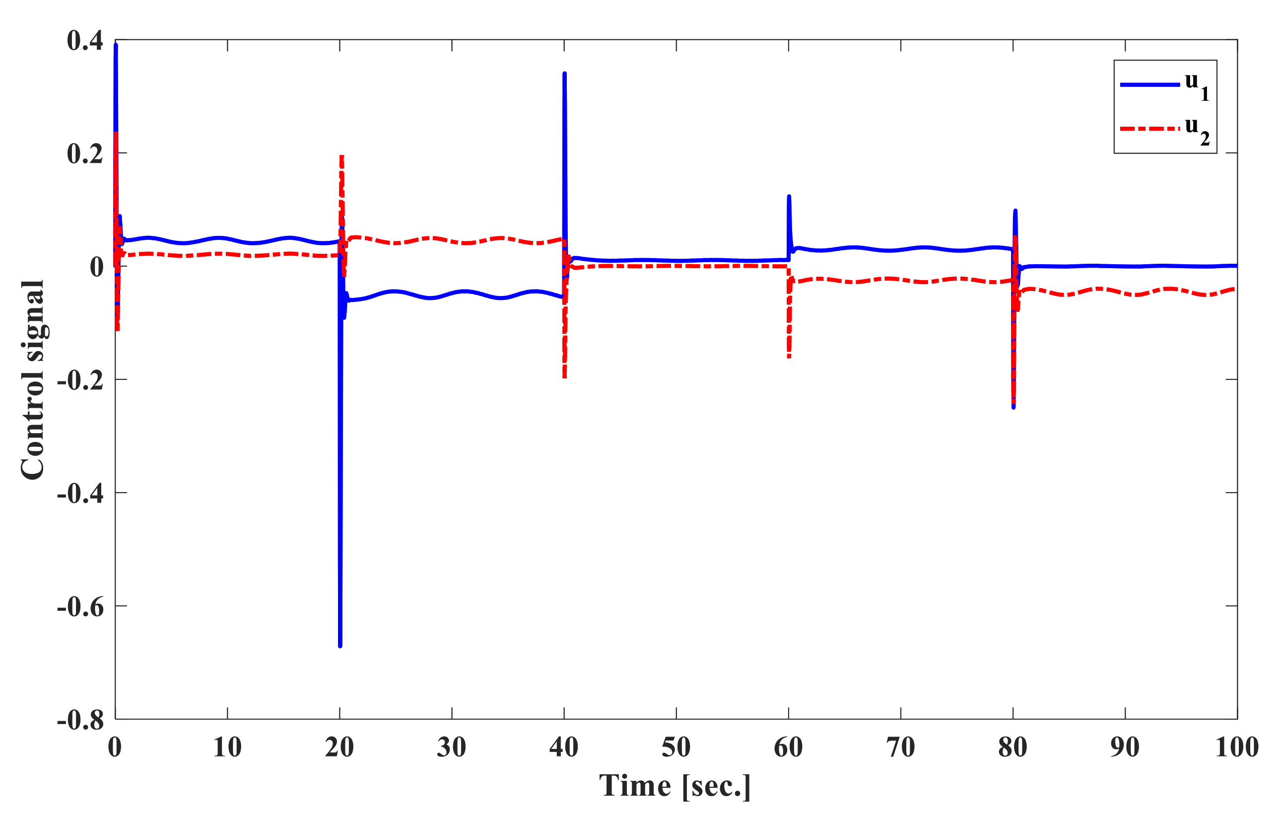
4.3. Simulation 3
5. Conclusions
Author Contributions
Funding
Conflicts of Interest
References
- Vijay, V.; James, C.; Paul, A.; Fouad, A. Power system control and stability; Wiley-IEEE Press: Hoboken, NJ, USA, 2019. [Google Scholar]
- Devendra, K. Techniques and Its Applications in Electrical Engineering; Springer: Berlin/Heidelberg, Germany, 2008. [Google Scholar]
- Fu, C.; Tan, W. Decentralized load frequency control for power systems with communication delays via active disturbance rejection. IET Gener. Transm. Distrib. 2018, 12, 1751–8687. [Google Scholar]
- Zhang, Y.; Yang, T. Decentralized switching control strategy for load frequency control in multi-area power systems with time delay and packet lose. IEEE Access 2020, 8, 15838–15850. [Google Scholar] [CrossRef]
- Guha, D.; Roy, P.K.; Banerjee, S. Load frequency control of interconnected power system using grey wolf optimization. Swarm Evol. Comput. 2016, 27, 97–115. [Google Scholar] [CrossRef]
- Anwar, M.N.; Pan, S. A new PID load frequency controller design method in frequency domain through direct synthesis approach. Electr. Power Energy Syst. 2015, 67, 560–569. [Google Scholar] [CrossRef]
- Farahani, M.; Ganjefar, S.; Alizadeh, M. PID controller adjustment using chaotic optimization algorithm for multi-area load frequency control. IET Control. Theory Appl. 2012, 6, 1984–1992. [Google Scholar] [CrossRef]
- Sonkar, P.; Rahi, O.P. Tuning of modified PID load frequency controller for interconnected system with wind power plant via IMC tuning method. In Proceedings of the 4th IEEE Uttar Pradesh Section International Conference on Electrical, Computer and Electronics, Mathura, India, 26–28 October 2017. [Google Scholar]
- Sahu, R.K.; Panda, S.; Rout, U.K. DE optimized parallel 2-DOF PID controller for load frequency control of power system with governor dead-band nonlinearity. Electr. Power Energy Syst. 2013, 49, 19–33. [Google Scholar] [CrossRef]
- Chen, H.; Ye, R.; Wang, X.; Lu, R. Cooperative control of power system load and frequency by using differential games. IEEE Trans. Control Syst. Technol. 2015, 23, 882–897. [Google Scholar] [CrossRef]
- Yousef, H.A.; AL-Kharusi, K.; Albadi, M.H.; Hosseinzadeh, N. Load frequency control of a multi-area power system: An adaptive fuzzy logic approach. IEEE Trans. Power Syst. 2014, 29, 1822–1830. [Google Scholar] [CrossRef]
- Zeng, G.Q.; Xie, X.Q.; Chen, M.R. An adaptive model predictive load frequency control method for multi-area interconnected power systems with photovoltaic generations. Electr. Power Energy Syst. 2017, 10, 1840. [Google Scholar] [CrossRef]
- Hao, Y.; Tan, W.; Li, D. Decentralized active disturbance rejection Control for LFC in deregulated environments. In Proceedings of the 33rd Chinese Control Conference, Nanjing, China, 28–30 July 2014. [Google Scholar]
- Saxena, S.; Hote, Y.V. Load frequency control in power systems via internal model control scheme and model-order reduction. IEEE Trans. Power Syst. 2013, 28, 2749–2757. [Google Scholar] [CrossRef]
- Rehiara, A.B.; Yorino, N.; Sasaki, Y.; Zoka, Y. An adaptive load frequency control based on least square method. Adv. Model. Control Wind Hydrog. 2020, 49, 220. [Google Scholar]
- Gheisarnejad, M.; Khooban, M.H. Design an optimal fuzzy fractional proportional integral derivative controller with derivative filter for load frequency control in power systems. Trans. Inst. Meas. Control 2019, 1, 1–19. [Google Scholar] [CrossRef]
- Daneshfar, F. Intelligent load-frequency control in a deregulated environment: Continuous-valued input, extended classifier system approach. IET Gener. Transm. Distrib. 2013, 7, 551–559. [Google Scholar] [CrossRef]
- Trip, S.; Cucuzzella, C.; De Persis, A.; Schaft, A.; Ferrara, A. Passivity-based design of sliding modes for optimal load frequency control. IEEE Trans. Control Syst. Technol. 2019, 27, 1893–1906. [Google Scholar] [CrossRef]
- Li, H.Y.; Shi, P.; Yao, D.Y.; Wu, L.G. Observer-based adaptive sliding mode control of nonlinear markovian jump systems. Automatica 2016, 64, 133–142. [Google Scholar] [CrossRef]
- Yang, B.; Yu, T.; Shu, H.; Yao, W.; Jiang, L. Sliding-mode perturbation observer-based sliding-mode control design for stability enhancement of multi-machine power systems. Trans. Inst. Meas. Control 2018, 41, 1418–1434. [Google Scholar] [CrossRef]
- Prasad, S.; Purwar, S.; Kishor, N. Non-linear sliding mode load frequency control in multi-area power system. Control Eng. Pract. 2017, 61, 81–92. [Google Scholar] [CrossRef]
- Mi, Y.; Fu, Y.; Wang, C.; Wang, P. Decentralized sliding mode load frequency control for multi-area power systems. IEEE Trans. Power Syst. 2013, 28, 4301–4309. [Google Scholar] [CrossRef]
- Sheetla, P.; Shubhi, P.; Nand, K. H-infinity based non-linear sliding mode controller for frequency regulation in interconnected power systems with constant and time-varying delays, IET Generation. Transm. Distrib. 2016, 10, 2771–2784. [Google Scholar]
- Xu, Y. A robust load frequency control scheme for power systems based on second order sliding mode and extended disturbance observer. IEEE Trans. Ind. Inform. 2018, 14, 3076–3086. [Google Scholar]
- Zheng, Y.; Liu, J.; Liu, X.; Fang, D.; Wu, L. Adaptive second order sliding mode control design for a class of nonlinear systems with unknown input. Math. Probl. Eng. 2015, 5, 1–7. [Google Scholar] [CrossRef][Green Version]
- Jianping, G. Load frequency control of a two area-power system with non-reheat turbines by SMC approach. J. Energy Power Eng. 2015, 9, 566–573. [Google Scholar] [CrossRef][Green Version]
- Mi, Y.; Fu, Y.; Li, D.; Wang, C.; Loh, P.C.; Wang, P. The sliding mode load frequency control for hybrid power system based on disturbance observer. Int. J. Electr. Power Energy Syst. 2016, 74, 446–452. [Google Scholar] [CrossRef]
- Dianwei, Q.; Shiwen, T.; Xiangjie, L. Load frequency control for micro hydro power plants by sliding mode and model order reduction. Automatika 2017, 56, 318–330. [Google Scholar]
- Dianwei, Q.; Shiwen, T.; Hong, L.; Xiangjie, L. Load frequency control by neural-network-based integral sliding mode for nonlinear power systems with wind turbines. Neurocomputing 2016, 173, 875–885. [Google Scholar]
- Le, N.M.B.; Van, V.H.; Nguyen, T.M.; Tsai, Y.W. Decentralized adaptive double integral sliding mode controller for multi-area power systems. Math. Probl. Eng. 2018, 2018, 1–11. [Google Scholar]
- Prasad, S.; Purwar, S.; Kishor, N. Load frequency regulation using observer based non-linear sliding mode control. Int. J. Electr. Power Energy Syst. 2019, 104, 178–193. [Google Scholar] [CrossRef]
- Jianping, G. Application of full order sliding mode control based on different areas power system with load frequency control. ISA Trans. 2019, 92, 23–24. [Google Scholar]
- Guo, J. Application of a novel adaptive sliding mode control method to the load frequency control. Eur. J. Control 2020, 12, 3050–3071. [Google Scholar] [CrossRef]
- Khargonekar, P.P.; Petersen, I.R.; Zhou, K. Robust stabilization of uncertain linear systems: Quadratic stabilizability and H∞ control theory. IEEE Trans. Autom. Control 1990, 35, 356–361. [Google Scholar] [CrossRef]
- Boyd, S.; Ghaoui, E.L.; Feron, E.; Balakrishna, V. Linear Matrix Inequalities in System and Control Theory; SIAM: Philadelphia, PN, USA, 1994. [Google Scholar]


| Parameter | ||||||
|---|---|---|---|---|---|---|
| Value for both areas | 20 s | 12 | 0.3 | 0.08 | 2.4 | 0.2545 |
| Parameter | ||||||
|---|---|---|---|---|---|---|
| Value for both areas | 20 | 120 | 0.3 | 0.08 | 2.4 | 0.5450 |
| Kinds of Controller | The Proposed SOISMC Approach | Different Sliding Mode Control Scheme For LFC | ||
|---|---|---|---|---|
| Parameters | Max.O.S | Max.O.S | ||
| 5 | 0.0090 | 105 | 0.0200 | |
| 6 | 0.0070 | 110 | 0.0150 | |
Publisher’s Note: MDPI stays neutral with regard to jurisdictional claims in published maps and institutional affiliations. |
© 2020 by the authors. Licensee MDPI, Basel, Switzerland. This article is an open access article distributed under the terms and conditions of the Creative Commons Attribution (CC BY) license (http://creativecommons.org/licenses/by/4.0/).
Share and Cite
Huynh, V.V.; Tran, P.T.; Minh, B.L.N.; Tran, A.T.; Tuan, D.H.; Nguyen, T.M.; Vu, P.-T. New Second-Order Sliding Mode Control Design for Load Frequency Control of a Power System. Energies 2020, 13, 6509. https://doi.org/10.3390/en13246509
Huynh VV, Tran PT, Minh BLN, Tran AT, Tuan DH, Nguyen TM, Vu P-T. New Second-Order Sliding Mode Control Design for Load Frequency Control of a Power System. Energies. 2020; 13(24):6509. https://doi.org/10.3390/en13246509
Chicago/Turabian StyleHuynh, Van Van, Phong Thanh Tran, Bui Le Ngoc Minh, Anh Tuan Tran, Dao Huy Tuan, Tam Minh Nguyen, and Phan-Tu Vu. 2020. "New Second-Order Sliding Mode Control Design for Load Frequency Control of a Power System" Energies 13, no. 24: 6509. https://doi.org/10.3390/en13246509
APA StyleHuynh, V. V., Tran, P. T., Minh, B. L. N., Tran, A. T., Tuan, D. H., Nguyen, T. M., & Vu, P.-T. (2020). New Second-Order Sliding Mode Control Design for Load Frequency Control of a Power System. Energies, 13(24), 6509. https://doi.org/10.3390/en13246509